04 August 2020
Repository ISTITUZIONALE
Multiple-Regression Method for Fast Estimation of Solar Irradiation and Photovoltaic Energy Potentials over Europe and Africa / Bocca, Alberto; Bergamasco, Luca; Fasano, Matteo; Bottaccioli, Lorenzo; Chiavazzo, Eliodoro; Macii, Alberto; Asinari, Pietro. - In: ENERGIES. - ISSN 1996-1073. - ELETTRONICO. - 11:12(2018), p. 3477.
Original
Multiple-Regression Method for Fast Estimation of Solar Irradiation and Photovoltaic Energy Potentials
over Europe and Africa
Publisher: Published DOI:10.3390/en11123477 Terms of use: openAccess Publisher copyright
(Article begins on next page)
This article is made available under terms and conditions as specified in the corresponding bibliographic description in the repository
Availability:
This version is available at: 11583/2720797 since: 2018-12-17T12:22:35Z
Article
Multiple-Regression Method for Fast Estimation of
Solar Irradiation and Photovoltaic Energy Potentials
over Europe and Africa
Alberto Bocca1 , Luca Bergamasco2 , Matteo Fasano2 , Lorenzo Bottaccioli1 , Eliodoro Chiavazzo2 , Alberto Macii1and Pietro Asinari2,*
1 Department of Control and Computer Engineering, Politecnico di Torino, 10129 Turin, Italy;
[email protected] (A.B.); [email protected] (L.B.); [email protected] (A.M.)
2 Department of Energy, Politecnico di Torino, 10129 Turin, Italy; [email protected] (L.B.);
[email protected] (M.F.); [email protected] (E.C.)
* Correspondence: [email protected]
Received: 15 November 2018; Accepted: 10 December 2018; Published: 13 December 2018
Abstract: In recent years, various online tools and databases have been developed to assess the potential energy output of photovoltaic (PV) installations in different geographical areas. However, these tools generally provide a spatial resolution of a few kilometers and, for a systematic analysis at large scale, they require continuous querying of their online databases. In this article, we present a methodology for fast estimation of the yearly sum of global solar irradiation and PV energy yield over large-scale territories. The proposed method relies on a multiple-regression model including only well-known geodata, such as latitude, altitude above sea level and average ambient temperature. Therefore, it is particularly suitable for a fast, preliminary, offline estimation of solar PV output and to analyze possible investments in new installations. Application of the method to a random set of 80 geographical locations throughout Europe and Africa yields a mean absolute percent error of 4.4% for the estimate of solar irradiation (13.6% maximum percent error) and of 4.3% for the prediction of photovoltaic electricity production (14.8% maximum percent error for free-standing installations; 15.4% for building-integrated ones), which are consistent with the general accuracy provided by the reference tools for this application. Besides photovoltaic potentials, the proposed method could also find application in a wider range of installation assessments, such as in solar thermal energy or desalination plants.
Keywords: solar energy; photovoltaic potential; renewable energy; fast energy analysis; sustainable development
1. Introduction
The world population is estimated to reach nearly 8.1 billion in 2040, with an average global economic growth of 3.4% per year. As a result, energy scenarios forecast a remarkable increase in global energy demand of about 30% by 2040 [1]. In line with the ratified agreements for worldwide sustainable development [2], a significant step up of renewables over conventional fossil fuels is expected in the global energy mix. The average net capacity addition per year of renewable energy is foreseen to grow steadily in the near future, led mainly by electricity production via solar photovoltaic (PV) conversion (see Figure1a).
2010 - 2016 0 20 40 60 80 100 120 140 160 180 Power capacity [GW] R C G N PV WIND OTHER 2017 - 2040 0 20 40 60 80 100 120 140 160 180 Power capacity [GW] R C G N PV WIND OTHER (a) (b)
Figure 1.(a) Average net capacity additions per year on the global power market by type (N: nuclear, G: gas, C: coal, R: renewables) according to the World Energy Outlook 2017 [1]. (b) Total in-plane solar irradiation for an equator-facing plane inclined 20◦from the horizontal (color bar units are in kWh/m2). Figure adapted (that is, cropped from original) from Reference [3], used under CC BY 4.0 license.
In recent years, the PV market in Europe has experienced a tremendous expansion, owing to the EU directive 2009/28/EC on the promotion of energy from renewable sources. Such initiative aims at fulfilling 20% of the overall energy needs of Europe with renewables by 2020 [4], and 27% by 2030 [5]. Considering that building-integrated installations have the advantage to preserve natural landscape with respect to large free-standing installations (PV farms), they have been promoted by local governments via specific policies, which led to a continuously increasing number of installations [6]. On the other hand, despite the outstanding potential in terms of solar energy and thus of sustainable electricity production [7], investments are still at the beginning in Africa [8]. In this sense, proper economic arguments on this potential would help to deploy investments, with beneficial effects particularly in rural areas, where no connection to the electric power grid is available. Photovoltaic systems could also favor the democratization of the energy availability [9], especially in Sub-Saharan Africa [10]. To promote and drive investments in Europe and Africa in this rapidly expanding market, one key aspect is the availability of fast and reliable screening tools for estimating: (i) the intensity of the available solar resource, which depends on the geographical location and climate; (ii) the potential energy output, which depends on the PV module technology, installation and local ambient conditions.
Methods for estimating the annual energy yield of PV systems can be classified into direct and indirect approaches [11]. The former evaluates the electrical energy output directly from the solar irradiation (i.e., insolation), whereas the latter obtains the energy output from the solar irradiation, ambient temperature, and some additional ancillary parameters [3,12]. The common starting point of these methods is a reliable measure or estimate of the available solar potential for specific geographical locations. In general, solar irradiation is best obtained via experimental measures by transducers (e.g., pyranometers and pyrheliometers in dedicated stations). However, this implies installation and monitoring difficulties in remote areas, especially those characterized by poorly developed technological access. Furthermore, such measurement stations are not suitable for collecting data in large-scale territories, because of their high capital and operating costs.
For this reason, a growing number of (online) tools and databases with solar irradiation data have been developed lately, for instance PVWatts [13], PVGIS [14], Global Atlas [15] or Solargis [16]. In particular, PVWatts is a web application implemented by the National Renewable Energy Laboratory (NREL) that can be used to predict the electricity generation from PV systems given the geographical position of the installation site and some technical details of the plant (e.g., size, module type, array type, losses, tilt, azimuth). This tool has been developed to be easily accessible and usable by both non-experts and advanced users. The prediction errors of the PVWatts model are claimed to be in the range±10% for annual energy totals [13]. PVGIS, instead, is an online calculator of potential electricity production by PV systems developed by the Joint Research Center (JRC) [17]. In addition to the annual electricity production, PVGIS is also capable to provide estimations of the monthly and hourly ones. The required inputs are again the geographical location of the PV system and its technological characteristics. The database used by PVGIS for solar radiation in Europe and Africa (see e.g., the total in-plane solar irradiation in Figure1b) demonstrated a mean bias error of about 2% against satellite data [17].
However, such online tools sometimes provide low-resolution data (i.e., in the range of only a few kilometers), which may be scattered and require multiple queries to the online databases in case of large-scale analysis. Thus, various models have been developed for forecasting the local solar resource using only the most widespread climatic data [18]. Both empirical and non-empirical models have been implemented for estimating monthly, daily, and hourly global solar irradiation [19,20]. While short-term estimations methods deserve greater attention [21,22] for dealing with the conversion efficiency [3,23], long-term estimations are essential to analyze possible investment scenarios with respect to the PV solar energy potential [24,25]. These can be obtained using either data pattern analysis [26,27] or physical modeling approaches [28,29].
In this work, we propose a simple yet effective model to estimate the yearly solar irradiation per unit area, only taking into account the latitude, altitude, and average temperature of a certain location as input parameters. The yearly PV potential output is then obtained considering the different climatic and technological factors affecting electricity production, namely the temperature, reflection, module, and installation efficiencies, as well as the non-optimal azimuthal angle of the module. This procedure is first formulated and then validated against well-established databases for both free-standing and building-integrated systems. This approach may be particularly beneficial when only scattered data of solar irradiation are available over large territories but high-resolution analysis would be required. Furthermore, the presented methodology—which is now implemented for Europe and Africa—does not require querying online databases and thus has the capability to operate offline.
The layout of this work is as follows. The proposed models for the yearly sum of global irradiation and PV energy potential are introduced in Section2. The parametrization of these models for Europe and Africa is reported in Section3, together with a comparison of the estimated solar irradiation and electricity generation by PV systems with those of a well-established online database, using standard error metrics. In Section4, the final conclusions are drawn and an outlook on the perspective developments and applications of the present work are given.
2. Methodology
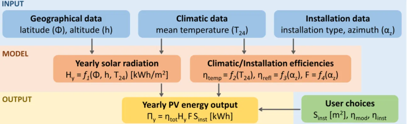
The aim of the proposed methodology is to provide: (i) a fast means for evaluating the global energy irradiation in locations where no or scattered data are available; (ii) a fast and easy-to-use screening tool for the preliminary assessment of the perspective PV energy yield over large territories. As sketched in Figure2, the approach relies on three basic and easily accessible data types, namely the latitude (φ), altitude above sea level (h), and average daily ambient temperature (T24) for a given
site. We remark that, for the purpose of the analysis, the average daytime temperature would be a more suitable parameter as it is most closely related to sunlight; however, this information is generally less accessible. Therefore, we useT24values because they are more easily retrievable for
implicitly, since wind, clouds, humidity, fog, pollution, or other environmental conditions indirectly affect the global energy irradiation estimate through the average daytime temperature. Additionally, system-dependent factors such as installation type (free-standing or building-integrated), azimuth of the module respect to the optimal orientation (αz), solar exposed surface (Sinst), PV module (ηmod), and installation (ηinst) efficiencies are also required for the final estimation of the yearly PV energy
output. The multiple-regression method allowed the correlation of these inputs with the yearly solar irradiation (Hy) and PV energy output (Πy) for the considered installation.
Yearly PV energy output Πy= ηtotHy F Sinst[kWh]
Yearly solar radiation
Hy= f1(Φ, h, T24) [kWh/m2] Geographical data latitude (Φ), altitude (h) Climatic data mean temperature (T24) Installation data
installation type, azimuth (αz)
Climatic/Installation efficiencies ηtemp = f2(T24), ηrefl= f3(αz), F = f4(αz)
INPUT
MODEL
OUTPUT User choices
Sinst[m2], ηmod, ηinst
Figure 2. Overview of the proposed methodology for fast estimation of solar irradiation and photovoltaic energy potential over large territories.
Source: Esri, DigitalGlobe, GeoEye, Earthstar Geographics, CNES/Airbus DS, USDA, USGS, AeroGRID, IGN, and the GIS User Community Figure 3. Randomly chosen geographical locations for the analysis (the full list of coordinates is reported in the AppendixA). The data set consists of 80 locations, 40 in Europe and 40 in Africa. Map source: ESRI World Imagery [30].
First, based on the three selected geodata types, the following general equation is found to provide an accurate estimation of the average yearly sum of global solar irradiation:
Hy=w1|φ|+w2h+w3T242 +w4|φ|T242 +w5. (1)
In the above equation, the latitudeφis considered in absolute value, meaning that the dependence ofHyon this parameter is symmetrical with respect to the equator. The model also reports that the
yearly sum of global solar irradiation depends linearly on the altitude of the selected location and quadratically on the average temperature. This evidence is physically meaningful, since insolation has been repeatedly found to rely on latitude [31], altitude [32], and climate conditions (e.g., average temperature) [33]; whereas, no effect of longitude (λ) is typically noticed. Finally,wi(i=1, ..., 5) are the
weights (or coefficients) of the polynomial model, which will be fitted in Section3over an extensive set of geographic locations throughout Europe and Africa (see Figure3).
Second, to predict the specific electrical output by a PV system at a given location, one must consider the various climatic and technological lossesψand the corresponding efficienciesη=1−ψ. In particular, we consider: (i) the efficiency resulting from losses due to temperature and low-irradiance effectsηtemp; (ii) the efficiency resulting from losses due to angular reflectance effectsηrefl; (iii) the
efficiency of the module technology itselfηmod, and (iv) the additional efficiency resulting from losses
due to system installationηinst (e.g., inverter and cables). The final correction factor applied to the
available solar insolation is the product of the aforementioned efficiencies, namely
ηtot=ηtempηreflηmodηinst. (2)
Among the various correlations available in the literature [34,35], here the temperature and low-irradiance efficiency is considered to have the following form [24]:
ηtemp=p1T242 +p2T24+p3, (3)
where the model coefficientspidepend on the installation type (free-standing or building-integrated)
and PV technology. Similarly, one of the possible correlations [36] to model the reflectance efficiency is a fourth-order polynomial using the azimuthal angle between the module orientation and either the South (northern hemisphere) or North (southern hemisphere) direction as independent variable [24]: ηrefl=q1α4z+q2α3z+q3α2z+q4αz+q5. (4)
Note that the model coefficientspi in Equation (3) andqi in Equation (4) will be obtained in
Section3by fitting the data of the geographic locations reported in Figure3. The remaining coefficients, namelyηmodandηinst, depend on user choice for the PV technology and installation, respectively.
One further correction of the PV energy output must be considered when non-optimal azimuthal angles of the PV installation are imposed. In fact,Hyrefers to the yearly sum of global solar irradiation
under optimal orientation of the PV module, namelyαz = 0. Usually, this mounting angle is not
always possible (especially in building-integrated installations), thus a correction factorF(αz)must be
included (note that the tilt angle of the modules may also be considered; however, in this work we assume optimal tilt). This scaling factor for the non-optimal azimuth can be obtained as a function of the azimuthal angle only as [24]
F(αz) =r1αz4+r2|α3z|+r3α2z+r4|αz|+r5, (5)
beingrithe model coefficients. In the next Section, we will show that proper parametrizations of this
model allow to obtain well-representative functions even for large geographical extents. Finally, the electrical energy output of the PV system is computed as
Πy=ηtotHyF Sinst, (6)
beingSinstthe net exposed surface of the installed modules.
In summary, as schematically depicted in Figure2, the proposed methodology for fast estimation of solar irradiation (Equation (1)) depends directly on geographical data (latitude, altitude) and indirectly on climatic data (average daytime temperature, which is implicitly influenced by wind, clouds, humidity, fog, pollution or other local environmental conditions). Instead, the estimation of
photovoltaic energy potential (Equations (2) and (6)) relies on both climatic data (average daytime temperature, Equation (3)) and installation characteristics of the considered PV system (photovoltaic technology, Equation (2); azimuth, Equations (4) and (5); installation type—that is building-integrated or free-standing).
3. Results
In this Section, the proposed methodology is tuned, validated, and then adopted to provide possible scenarios of the yearly PV production over large territories in Europe and Africa. First, the yearly sum of global solar irradiation is obtained according to Equation (1), which requires as inputs the latitudeφ, the altitudehand the mean temperatureT24for a given geographical location.
Then, the temperature and reflectance efficiencies are computed according to Equations (3) and (4) for optimal tilt and azimuthal angles of the modules. These efficiencies are then combined with the user-defined efficienciesηmodandηinst, to compute the total efficiencyηtotaccording to Equation (2).
The yearly electrical energy output is eventually estimated via Equation (6), based on the net surface of the installed PV modules. The analysis is finally carried out also for module installations that present non-optimal azimuthal angles, by considering the correction factorF(αz).
3.1. Solar Irradiation Model
The model coefficients for Equation (1) are fitted to a random set of 80 different geographical locations in Europe and Africa, see Figure3and TablesA1andA2, with latitudes covering a range from about 60◦to−30◦. Note that the exact geographical coordinates have been chosen based on the availability of the required data, so they do not generally coincide with the center of the indicated cities. These cities are indeed indicated as the most significant nearby location to the considered geographical point. The altitude, average temperature in the 24 h and the yearly sum of global solar irradiation for each location are extracted from the online database PVGIS [37] of the Joint Research Centre [17,38,39]. The solar irradiation database of PVGIS is based on data records of the Satellite Application Facility on Climate Monitoring (CM-SAF) [40]. The average local temperature (T24) is provided by the interactive
map, which covers Europe and part of the Northern Africa. All the temperature data for the locations in Africa with latitude lower than 32.5◦are obtained from Berkeley Earth™[41]. TheHyvalues are
extracted from the PVGIS database considering both optimal azimuthal angle and optimal tilt angle. The full set of data for these 80 random locations is split in two different subsets, namely a training and a validation set. The model coefficients of Equation (1) are initially fitted on the training data set; then, the best-fitted model is used to predict the responses for the observations in the second data set (the validation one), which provides an unbiased evaluation of the model fitting. Here, the training data set is taken as 70% (i.e., 56 locations) of the whole data set; whereas, the validation one includes 24 locations. The training/validation process is iteratively repeated 10,000 times, with a random distribution of locations in the two subsets, and standard error metrics are computed with respect to theHyvalues provided by the PVGIS tool [42]. The distribution of the mean absolute percent error
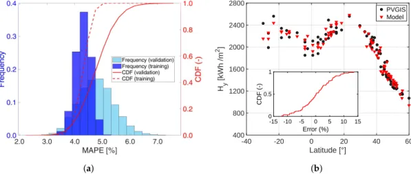
(MAPE) for the 10,000 repetitions is reported in Figure4a, for both the training and the validation steps. The MAPE distribution shows a Gaussian shape, with average values equal to 4.3% (training) and 4.9% (validation).
The fitted coefficients of Equation (1) per each training step are averaged over the 10,000 repetitions, and the resulting mean values and standard deviations are reported in Table1, where units forw1and
w4are indeed given per degree of latitude (the unit for latitude is the decimal degree, as recommended
by ISO 31, instead of using degrees, minutes and seconds [43]). These optimal coefficients are then used to predictHyfor the 80 considered locations in Europe and Africa. The predicted global sum
of solar irradiation is compared to that provided by the PVGIS tool, and the relative percent error is reported in the last column of TablesA1and A2. Figure4b shows a graphical comparison between theHyvalues obtained by the proposed model (Equation (1) with the optimal coefficients in Table1)
irradiation for Europe (from about 60◦to 37◦latitude) and Africa (from about 37◦to−30◦latitude) can be clearly appreciated; nevertheless, no systematic errors with the latitude are noticeable. Results show that the maximum relative error of the model prediction is 13.6% in absolute value, which is within the standard range of estimation errors for the yearly global irradiation. For instance, Solargis [44] reports a data accuracy in the range of±4% to±8% for the global horizontal irradiation, and±8% to±15% for the direct normal irradiation [45]. The inset of Figure4b, presents the cumulative distribution function of the percent error between the predicted and the PVGIS values ofHy. The MAPE is 4.4% and the
normalized root mean square error (NRMSE) in percentage is 5.5%. These errors are similar to the ones typically obtained in other solar irradiation models from the literature. For example, methodologies based on artificial neural networks or inverse distance weighting algorithm have shown mean absolute percent errors equal to 5.9%, 3.4% and 4.3% at a nationwide level (Malaysia [46], Indonesia [47], and Taiwan [48], respectively). Notably, such discrepancies are all consistent with investors requests, namely average errors within 5% in prediction accuracy [49].
(a) -40 -20 0 20 40 60 Latitude [°] 400 800 1200 1600 2000 2400 2800 Hy [kWh / m 2] PVGIS Model -15 -10 -5 0 5 10 15 Error (%) 0 0.5 1 CDF (-) (b)
Figure 4. (a) Distribution of the mean absolute percent error (MAPE) between the PVGIS and the predicted values of Hy, for the 10,000 repetitions of the training/validation process for the coefficients of Equation (1). Red lines refer to the cumulative distribution functions of the MAPE values. (b) Distribution of Hy for the 80 considered locations in Europe and Africa: comparison between PVGIS data (black dots) and estimations by Equation (1) with the optimal coefficients in Table1(red triangles). Note that the maximum average yearly sum of global solar irradiation is found at the Tropic of Cancer and Capricorn (±23◦latitude). In the inset, the cumulative distribution function of the percent estimation errors is shown.
Table 1. Model coefficients of Equation (1) obtained by the (training/validation) fitting procedure on the data sets in TablesA1andA2. The standard deviation indicates the variability of the fitted coefficients in the 10,000 different training sets. Note that, in Equation (1), the latitude is intended in decimal degrees.
Parameter Average Value Standard Deviation
w1 [kWh·m−2] −21.569 ±2.073
w2 [kWh·m−3] 0.137 ±0.031
w3 [kWh·m−2·◦C−2] −0.421 ±0.133 w4 [kWh·m−2·◦C−2] 0.071 ±0.003
w5 [kWh·m−2] 2119.345 ±108.680
This evidence shows that the number of chosen locations is sufficient to train adequate values of wi(i=1, ..., 5) coefficients and, therefore, that an accurately representative model for the yearly sum of
3.2. PV Energy Model (Optimal Azimuth)
The proposed methodology is now applied to estimate the potential electrical energy output by PV system installations for the whole set of considered locations. Initially,Hyand thusΠyare
computed considering installations with optimal tilt and azimuth, namelyαz = 0 and thusF = 1,
and crystalline silicon solar cells. The methodology is implemented in MATLAB®, resulting in a simple and fast algorithm that can be straightforwardly applied for the analysis of large data sets.
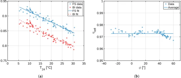
First, the model coefficients for the temperature and low-irradiance efficiency in Equation (3) are obtained by fitting the values extracted from PVGIS tool over the 80 locations in Europe and Africa. Best-fitted values for free-standing and building-integrated installations are listed in Table2. The coefficients of determination of these fittings, that is R2 = 0.92 (free-standing) and R2 = 0.90
(building-integrated), demonstrate that Equation (3) is an accurate correlation betweenηtempand
T24, as also evident in Figure5a. Second, the reflectance efficiency of Equation (4) is fitted on the
80 European and African locations as well. Since, in this case, we consider optimal azimuthal angle, Equation (4) simplifies toηrefl=q5, beingq5=0.972 the best-fitted value. As reported in Figure5b,
theηreflvalues from the PVGIS tool range from 0.967 to 0.978, namely within a±0.6% fromηrefl=0.972.
In fact,ηrefldemonstrates only a slight dependence on latitude.
0 5 10 15 20 25 30 35 T24 [°C] 0.75 0.8 0.85 0.9 0.95 temp FS data BI data FS fit BI fit (a) -40 -20 0 20 40 60 [°] 0.95 0.96 0.97 0.98 0.99 1 refl Data Average (b)
Figure 5. (a) Temperature and low-irradiance efficiency (ηtemp) as a function of the average daily
ambient temperature (T24) for the given locations: best-fitted models of Equation (3) (lines) are
compared with the values taken from the PVGIS tool (dots) for the 80 locations in Europe and Africa shown in Figure3. Crystalline silicon solar cells are considered. Free-standing (FS) installations are depicted in blue; whereas, building-integrated (BI) installations in red. (b) Reflectance efficiency (ηrefl)
as a function of the latitudeφfor the 80 locations in Europe and Africa: the values taken from the
PVGIS tool (dots) and their average value (line) are shown.
Table 2. Coefficients of the model for the temperature efficiency in Equation (3) fitted over the 80 considered locations in Europe and Africa (see Figure3). The reported values refer to crystalline silicon solar cells in either free-standing or building-integrated installations.
Parameter Free-Standing Building-Integrated p1 [◦C−2] −1.014×10⁻⁶ 2.757×10⁻⁵ p2 [◦C−1] −3.430×10⁻³ −4.598×10⁻³
p3 [−] 9.484×10⁻¹ 9.114×10⁻¹
TheΠy values are finally computed by Equation (6), considering an indicative efficiency for
the crystalline silicon solar cells equal toηmod =0.25 [50], a system installation efficiency equal to
Europe and Africa are compared to those provided by PVGIS tool, and the relative percent error is reported in Figure6a,b (free-standing installations), and in Figure6c,d (BI installations), respectively. Results show that the maximum relative error for FS installations is 14.8% in absolute value, MAPE is 4.3% and NRMSE is 5.5%. Similar errors are obtained for BI solutions, namely a maximum relative error equal to 15.4% in absolute value, MAPE equal to 4.3% and NRMSE to 5.5%. These values are essentially coherent with the prediction errors ofHydiscussed in the previous Section, which therefore represent
the main source of uncertainty in the Πy estimation. These uncertainties are consistent with the
general accuracy provided by other tools for estimating the PV potential throughout large territories. For example, PVWatts tool shows errors as high as±10% for annual PV electricity production, with actual performance in a specific year up to±20% respect to long-term average [13]. These uncertainties are also similar to those indicated by JRC (i.e., from−20% to+5%) when the effect of irradiation and temperature on PV module performance are both considered [3].
-20 -10 0 10 20 30 40 50 [°] -40 -20 0 20 40 60 [°] -15 -10 -5 0 5 10 15 y error [%] (a) (b) -20 -10 0 10 20 30 40 50 [°] -40 -20 0 20 40 60 [°] -15 -10 -5 0 5 10 15 y error [%] (c) (d)
Figure 6. (a) Percent error between the current model predictions of Equation (6) and the values extracted from the PVGIS tool for the yearly electrical energy output (Πy) of FS PV systems over the 80 considered locations in Europe and Africa. Results are reported as a function of the latitude (φ) and
longitude (λ), as well as in the form of (b) error distribution. (c) Percent error between the current
model predictions and the values extracted from the PVGIS tool for the yearly electrical energy output of BI PV systems. Results are reported as function of latitude (φ) and longitude (λ), as well as in the
3.3. Effect of Non-Optimal Azimuth
In this Section we analyze the effect of non-optimal azimuthal angles on the reflectance efficiency ηreflof Equation (4) and on the scaling factorF(αz)of Equation (5) for various geographical locations
in Europe and Africa. The locations are specifically selected to be representative of the whole extent of each continent, namely maximum, minimum, and intermediate latitudes. Using this criterion, the following spots are chosen from the data set: St. Petersburg (Russia), Edinburgh (UK), Rome (Italy) and Sevilla (Spain) for Europe; Rabat (Morocco), Aswan (Egypt), Karthoum (Sudan) and Kampala (Uganda) for Africa. Note that the selected spots also differ significantly in longitude; however, no appreciable effect of this latter parameter has been noticed in the analysis. The raw data for the reflectance efficiency and insolation is obtained for each location using standard queries to the online PVGIS tool, for azimuthal angles varying in the range−90◦ ≤αz ≤90◦.
The results are shown in Figure7a,b, where we also compare the solution given by Equations (4) and (5), respectively. The parametrization of these two latter equations was previously obtained for Italy, using the raw data of seven cities throughout the peninsula for the reflectance efficiency and the only data of Rome for the scaling factor [24]. We note that the parametrization for Italy gives well-representative curves also for the other locations in Europe: the maximum relative error is 2.1% on the reflectance efficiency and 13.8% on the scaling factor at the maximum azimuthal angles considered (±90◦). We can then assert that, given the geographical location of Italy at intermediate continental latitudes, this parametrization can be assumed to be representative also for Europe—and the coefficients are reported in Table3. On the other hand, the results for Africa require a specific treatment, as the decrease in latitude towards the equator significantly modifies both the reflectance efficiency and the scaling factor with respect to those of the European spots. We then proceed with a new parametrization of the models by regression, using the data of the four considered locations in Africa. We obtain the coefficients reported in Table3. In this case, the maximum relative error is 0.3% on the reflectance efficiency and 6.4% on the scaling factor at the maximum azimuthal angles. Considering thatαz = ±90◦is the most unfavorable and limiting situation for an installation, the
proposed models provide acceptable approximations for the reflectance efficiency and scaling factor. In particular, according to the results obtained, the parametrization for Europe can be adopted in the range of latitudes 37◦≤φ≤60◦, while that for Africa fromφ=37◦to the equator (φ=0◦). Symmetry applies for locations in Africa below the equator (negative latitudes).
-90 -75 -60 -45 -30 -15 0 15 30 45 60 75 90 z [°] 0.950 0.955 0.960 0.965 0.970 0.975 refl
[-] St. Petersburg (RU)Edinburgh (UK) Rome (Italy) Seville (Spain) Rabat (Marocco) Aswan (Egypt) Karthoum (Sudan) Kampala (Uganda) Model of Eq. (4) for Europe Model of Eq. (4) for Africa
(a) -90 -75 -60 -45 -30 -15 0 15 30 45 60 75 90 z [°] 0.82 0.84 0.86 0.88 0.90 0.92 0.94 0.96 0.98 1.00 F( z ) [-] St. Petersburg (RU) Edinburgh (UK) Rome (Italy) Seville (Spain) Rabat (Marocco) Aswan (Egypt) Karthoum (Sudan) Kampala (Uganda) Model of Eq. (5) for Europe Model of Eq. (5) for Africa
(b)
Figure 7.Results obtained from the PVGIS tool for the reflectance efficiency (a) and scaling factor (b) for the selected locations in Europe (circles) and Africa (triangles). The solid lines correspond to the model in Equation (4) in (a) and Equation (5) in (b) for Europe (red) and Africa (yellow), with the model coefficients reported in Table3for the two cases.
Table 3.Coefficients of the model for the reflectance efficiencyηreflin Equation (4) and for the scaling
factorF(αz)in Equation (5) for Europe as originally reported for Italy in Ref. [24], and those obtained for Africa in the present work.
ηrefl F(αz)
Europe Africa Europe Africa
q1 −2.038×10⁻¹¹ −1.219×10⁻¹¹ r1 3.729×10⁻⁹ 1.437×10⁻⁹ q2 −3.027×10⁻¹⁰ −4.317×10⁻¹¹ r2 −3.463×10⁻⁷ −1.002×10⁻⁷ q3 −1.193×10⁻⁶ −2.690×10⁻⁷ r3 −1.274×10⁻⁵ −9.295×10⁻⁶ q4 8.264×10⁻⁷ 1.512×10⁻⁷ r4 −1.650×10⁻⁴ 2.933×10⁻⁵
q5 9.722×10⁻¹ 9.734×10⁻¹ r5 1 1
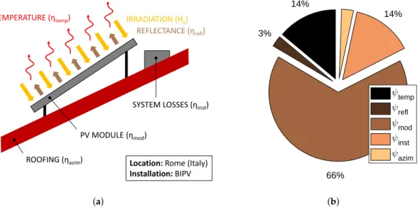
An example application of the proposed models and related analysis is reported in Figure8a,b for a BI installation in the city of Rome (Italy), which has azimuthal angleαz=35◦,ηmod=0.25 for
crystalline silicon solar cells [50],ηinst =0.84 and unitary exposed surface. The main contribution to
the total losses is given by the module efficiency, then by temperature and installation losses. Note that the losses due to reflectance effects and azimuthal angle contribute only for a small share on the total losses. For Europe, a similarly small contribution of the reflectance losses would be obtained for any azimuthal angle, as they consist in any case of a few percent (see Figure7a). The contribution of losses due to the azimuthal angle can be expected to be more consistent for large azimuthal angles, e.g., forαz =±60◦, where losses could reach nearly 10% (see Figure7b). For Africa, both contributions
to the total losses tend to be smaller for any azimuth.
ROOFING (ηazim)
PV MODULE (ηmod)
SYSTEM LOSSES (ηinst)
REFLECTANCE (ηrefl)
IRRADIATION (Hy)
TEMPERATURE (ηtemp)
Location:Rome (Italy) Installation:BIPV (a) 14% 3% 66% 14% 3% temp refl mod inst azim (b)
Figure 8. (a) Sample analysis of the various contributions to the total losses (η = 1−ψ) for a
building-integrated installation (BIPV) in the city of Rome (Italy) with unitary exposed surface. The azimuthal angle considered isαz = 35◦ (ψazim losses), the module efficiency isηmod = 0.25
(ψmodlosses) for crystalline silicon solar cells [50], and the installation efficiency isηinst=0.84 (ψinst
losses). (b) The results obtained show that the main contribution to the total losses depends on the choice of the module technology.
4. Concluding Remarks
In this work, we have proposed a simple methodology for a fast estimation of the yearly sum of solar irradiation in Europe and Africa and the resulting potential PV energy output. The model thus generated is intended to provide: (i) high spatial (continuous) resolution and (ii) a fast means for pre-screening of the PV potential over large-scale territories for any investor. In fact, the presented
method relies on just a small set of input parameters. For instance, estimation of the yearly sum of global solar irradiation requires only the knowledge of a few basic geodata, such as latitude, altitude, and average daily temperature. One such tool operates offline and provides a much faster screening than systematic calls to online databases, and can be easily implemented with just a few lines of code.
Limitations of this work include the lack of information at local level, for instance, about the shading effect of buildings or other elements nearby, as well as horizon height. Thus, the reported tool should be considered as a fast (macroscopic) screening of the solar and PV potentials over large-scale territories with tolerable errors in the range±5%, which should then be followed by a more accurate (microscopic) analysis considering also local elements for a limited set of locations. Furthermore, both the solar irradiation and the potential photovoltaic electricity generation are here estimated on an annual basis, namely they consider the cumulative value over the average year. The reason is that the yearly electricity output is a standard figure of merit needed to assess the techno-economic feasibility of a possible photovoltaic system in a given location [31]. Clearly, this information would not be enough to size the whole photovoltaic system, since detailed estimations of daily and hourly variability are required to design, for example, the energy storage system [51]. In perspective, our multiple-regression model could be further improved to consider daily variability as well, for instance by including well-established models from the literature [52].
This approach may find application in the design of micro-grids [53], polygeneration systems [54], BI PV solutions [55] or flexible storage photovoltaic systems [56]. Furthermore, this methodology could also support the large-scale potential assessment of sustainable technologies other than photovoltaics, for example, solar thermal systems [57], solar greenhouses or dryers for food production or conservation [58], and desalination plants driven by solar source [59].
Author Contributions:A.B. conceived the idea of this study. A.B., with help of L.B. (Luca Bergamasco) and M.F., performed the computations, analyzed the results and wrote the manuscript. L.B. (Lorenzo Bottaccioli) prepared the training and validation data sets. A.M., E.C. and P.A. provided methodological support and supervised the study. All authors have read and approved the final version of the manuscript.
Funding:This research received no external funding.
Acknowledgments:Computational resources provided by HPC@POLITO, a project of Academic Computing of the Department of Control and Computer Engineering (DAUIN) at Politecnico di Torino (http://hpc.polito.it).
Conflicts of Interest:The authors declare no conflict of interest. Abbreviations
The following abbreviations are used in this manuscript:
PV Photovoltaic
BIPV Building-Integrated Photovoltaic
PVGIS Photovoltaic Geographic Information System JRC Joint Research Centre (European Commission) CM-SAF Satellite Application Facility on Climate Monitoring MAPE Mean Absolute Percent Error
Appendix A
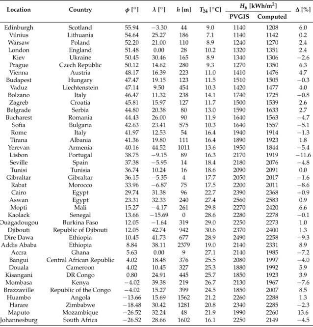
Table A1. Locations in Europe and Africa considered to train and validate the multiple-regression method. For each location, latitude (φ), longitude (λ), altitude (h), and mean temperature over 24 h
(T24) are reported. The yearly sum of the global solar irradiation (Hy) as obtained from the PVGIS
tool [37] and the proposed estimator are compared. The last column reports the relative error of the estimates with respect to the PVGIS data. Note that the exact geographical coordinates have been chosen based on the availability of the required data, and the indicated cities/places represent the most significant locations nearby the considered geographical points.
Location Country φ[◦] λ[◦] h[m] T24[◦C] Hy[kWh/m 2] ∆[%] PVGIS Computed Edinburgh Scotland 55.94 −3.30 44 9.0 1140 1208 6.0 Vilnius Lithuania 54.64 25.27 186 7.1 1140 1142 0.2 Warsaw Poland 52.20 21.00 110 8.9 1240 1270 2.4 London England 51.48 0.00 28 10.2 1320 1351 2.4 Kiev Ukraine 50.45 30.46 165 8.9 1340 1306 −2.6
Prague Czech Republic 50.12 14.62 280 9.3 1270 1350 6.3
Vienna Austria 48.17 16.39 223 11.0 1410 1476 4.7 Budapest Hungary 47.47 19.15 123 11.5 1510 1505 −0.3 Vaduz Liechtenstein 47.14 9.50 454 10.3 1420 1477 4.0 Bolzano Italy 46.47 11.32 238 14.1 1740 1725 −0.8 Zagreb Croatia 45.81 15.97 127 11.7 1500 1539 2.6 Belgrade Serbia 44.80 20.38 80 13.0 1590 1633 2.7 Bucharest Romania 44.43 26.00 90 11.9 1640 1563 −4.7 Sofia Bulgaria 42.63 23.41 575 10.3 1640 1557 −5.1 Rome Italy 41.97 12.53 54 16.4 1940 1914 −1.3 Tirana Albania 41.36 19.80 111 16.4 1890 1923 1.8 Yerevan Armenia 40.16 44.52 1011 13.6 1950 1844 −5.4 Lisbon Portugal 38.75 −9.15 89 16.3 2170 1919 −11.6 Seville Spain 37.38 −5.95 14 18.4 2180 2076 −4.8 Tunisi Tunisia 36.74 10.24 16 18.6 2090 2091 0.0 Gibraltar Gibraltar 36.15 −5.35 4 17.7 2050 2017 −1.6 Rabat Morocco 33.96 −6.87 75 17.5 2200 2011 −8.6 Cairo Egypt 29.74 31.38 96 22.7 2390 2368 −0.9 Aswan Egypt 23.31 32.33 240 27.4 2560 2583 0.9 Mopti Mali 15.27 −4.17 261 29.8 2270 2420 6.6 Kaolack Senegal 13.66 −15.69 0 28.6 2280 2278 −0.1
Ouagadougou Burkina Faso 12.05 −1.64 319 29.0 2250 2273 1.0
Djibouti Republic of Djibouti 12.05 42.74 942 30.6 2370 2400 1.3
Dire Dawa Ethiopia 10.45 41.73 677 28.9 2490 2258 −9.3
Addis Ababa Ethiopia 8.84 38.11 2379 19.0 2140 2331 8.9
Accra Ghana 5.63 0.00 9 27.1 2140 1985 −7.2
Bangui Central African Republic 4.02 18.48 376 25.5 2080 1997 −4.0
Douala Cameroon 4.02 10.45 327 25.3 1880 1992 5.9
Kisangani DR Congo 0.80 24.91 445 25.7 1850 1923 3.9
Mombasa Kenya −4.02 39.38 219 26.7 2130 1967 −7.6
Brazzaville Republic of the Congo −4.02 15.27 399 24.5 1850 2007 8.5
Huambo Angola −13.66 15.69 1562 21.2 2260 2288 1.3
Harare Zimbabwe −18.48 30.42 1281 20.8 2340 2285 −2.3
Maputo Mozambique −26.52 32.24 48 21.9 1990 2260 13.6
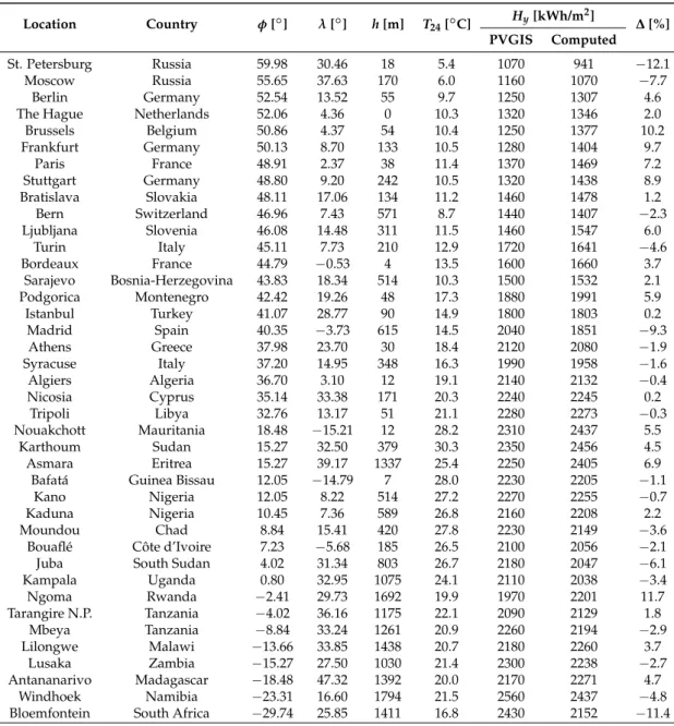
Table A2. Locations in Europe and Africa considered to train and validate the multiple-regression method. For each location, latitude (φ), longitude (λ), altitude (h), and mean temperature over 24 h
(T24) are reported. The yearly sum of the global solar irradiation (Hy) as obtained from the PVGIS
tool [37] and the proposed estimator are compared. The last column reports the relative error of the estimates with respect to the PVGIS data. Note that the exact geographical coordinates have been chosen based on the availability of the required data, and the indicated cities/places represent the most significant locations nearby the considered geographical points.
Location Country φ[◦] λ[◦] h[m] T24[◦C] Hy[kWh/m 2] ∆[%] PVGIS Computed St. Petersburg Russia 59.98 30.46 18 5.4 1070 941 −12.1 Moscow Russia 55.65 37.63 170 6.0 1160 1070 −7.7 Berlin Germany 52.54 13.52 55 9.7 1250 1307 4.6
The Hague Netherlands 52.06 4.36 0 10.3 1320 1346 2.0
Brussels Belgium 50.86 4.37 54 10.4 1250 1377 10.2 Frankfurt Germany 50.13 8.70 133 10.5 1280 1404 9.7 Paris France 48.91 2.37 38 11.4 1370 1469 7.2 Stuttgart Germany 48.80 9.20 242 10.5 1320 1438 8.9 Bratislava Slovakia 48.11 17.06 134 11.2 1460 1478 1.2 Bern Switzerland 46.96 7.43 571 8.7 1440 1407 −2.3 Ljubljana Slovenia 46.08 14.48 311 11.5 1460 1547 6.0 Turin Italy 45.11 7.73 210 12.9 1720 1641 −4.6 Bordeaux France 44.79 −0.53 4 13.5 1600 1660 3.7 Sarajevo Bosnia-Herzegovina 43.83 18.34 514 10.3 1500 1532 2.1 Podgorica Montenegro 42.42 19.26 48 17.3 1880 1991 5.9 Istanbul Turkey 41.07 28.77 90 14.9 1800 1803 0.2 Madrid Spain 40.35 −3.73 615 14.5 2040 1851 −9.3 Athens Greece 37.98 23.70 30 18.4 2120 2080 −1.9 Syracuse Italy 37.20 14.95 348 16.3 1990 1958 −1.6 Algiers Algeria 36.70 3.10 12 19.1 2140 2132 −0.4 Nicosia Cyprus 35.14 33.38 171 20.3 2240 2245 0.2 Tripoli Libya 32.76 13.17 51 21.1 2280 2273 −0.3 Nouakchott Mauritania 18.48 −15.21 12 28.2 2310 2437 5.5 Karthoum Sudan 15.27 32.50 379 30.3 2350 2456 4.5 Asmara Eritrea 15.27 39.17 1337 25.4 2250 2405 6.9
Bafatá Guinea Bissau 12.05 −14.79 7 28.0 2230 2205 −1.1
Kano Nigeria 12.05 8.22 514 27.2 2270 2255 −0.7
Kaduna Nigeria 10.45 7.36 589 26.8 2160 2208 2.2
Moundou Chad 8.84 15.41 420 27.8 2230 2149 −3.6
Bouaflé Côte d’Ivoire 7.23 −5.68 185 26.5 2100 2056 −2.1
Juba South Sudan 4.02 31.34 803 26.7 2180 2047 −6.1
Kampala Uganda 0.80 32.95 1075 24.1 2110 2038 −3.4 Ngoma Rwanda −2.41 29.73 1692 19.9 1970 2201 11.7 Tarangire N.P. Tanzania −4.02 36.16 1175 22.1 2090 2129 1.8 Mbeya Tanzania −8.84 33.24 1261 20.9 2260 2194 −2.9 Lilongwe Malawi −13.66 33.85 1438 20.7 2180 2260 3.7 Lusaka Zambia −15.27 27.50 1030 21.4 2300 2238 −2.7 Antananarivo Madagascar −18.48 47.32 1392 20.0 2170 2271 4.7 Windhoek Namibia −23.31 16.60 1794 21.5 2560 2437 −4.8
Bloemfontein South Africa −29.74 25.85 1411 16.8 2430 2152 −11.4
References
1. IEA World Energy Outlook 2017. Available online:http://www.iea.org/weo/(accessed on 14 June 2018). 2. Kyoto Protocol to the United Nations Framework Convention on Climate Change; U.N. Doc FCCC/CP/1997/7/ Add.1, 37 I.L.M. 22; Kyoto, Japan, 1998. Available online:http://www.globaldialoguefoundation.org/files/ ENV.2009-jun.unframeworkconventionclimate.pdf(accessed on 11 December 2018).
3. Huld, T.; Gracia Amillo, A.M. Estimating PV Module Performance over Large Geographical Regions: The Role of Irradiance, Air Temperature, Wind Speed and Solar Spectrum. Energies2015,8, 5159–5181. [CrossRef]
4. Directive 2009/28/EC of the European Parliament and of the Council, 2009. Available online:http://data. europa.eu/eli/dir/2009/28/oj(accessed on 11 December 2018).
5. Proposal for a Directive COM 2016/767/F2 of the European Parliament and of the Council, 2016. Available online: https://ec.europa.eu/transparency/regdoc/rep/1/2016/EN/COM-2016-767-F2-EN-MAIN-PART-1.PDF(accessed on 11 December 2018).
6. Martínez-Rubio, A.; Sanz-Adan, F.; Santamaría-Peña, J.; Martínez, A. Evaluating solar irradiance over facades in high building cities, based on LiDAR technology. Appl. Energy2016,183, 133–147. [CrossRef] 7. Numbi, B.P.; Malinga, S.J. Optimal energy cost and economic analysis of a residential grid-interactive solar
PV system-case of eThekwini municipality in South Africa. Appl. Energy2017,186, 28–45. [CrossRef] 8. Micangeli, A.; Del Citto, R.; Santori, S.G.; Gambino, V.; Kiplagat, J.; Viganò, D.; Poli, D.; Fioriti, D.;
Del Citto, R.; Kiva, I.N. Energy Production Analysis and Optimization of Mini-Grid in Remote Areas: The Case Study of Habaswein, Kenya.Energies2017,10, 2041. [CrossRef]
9. International Renewable Energy Agency (IRENA). Solar PV in Africa: Costs and Markets, 2016. Available online: https://www.irena.org/-/media/Files/IRENA/Agency/Publication/2016/IRENA_Solar_PV_ Costs_Africa_2016.pdf(accessed on 11 December 2018).
10. Quansah, D.A.; Adaramola, M.S.; Mensah, L.D. Solar Photovoltaics in sub-Saharan Africa—Addressing Barriers, Unlocking Potential.Energy Procedia2016,106, 97–110. [CrossRef]
11. Rus-Casas, C.; Aguilar, J.D.; Rodrigo, P.; Almonacid, F.; Pérez-Higueras, P.J. Classification of methods for annual energy harvesting calculations of photovoltaic generators. Energy Convers. Manag.2014,78, 527–536. [CrossRef]
12. Yousif, J.H.; Kazem, H.A.; Boland, J. Predictive models for photovoltaic electricity production in hot weather conditions. Energies2017,10, 971. [CrossRef]
13. Dobos, A.P.PVWatts Version 5 Manual; Technical Report; National Renewable Energy Laboratory (NREL): Golden, CO, USA, 2014.
14. Šúri, M.; Huld, T.A.; Dunlop, E.D. PV-GIS: A web-based solar radiation database for the calculation of PV potential in Europe.Int. J. Sustain. Energy2005,24, 55–67. [CrossRef]
15. International Renewable Energy Agency (IRENA). Global Atlas for Renewable Energy: Overview of Solar and Wind Maps, 2014. Available online:https://www.irena.org/-/media/Files/IRENA/Agency/ Publication/2014/GA_Booklet_Web.pdf(accessed on 11 December 2018).
16. SOLARGIS. Available online:https://solargis.info/(accessed on 14 June 2018).
17. Huld, T.; Müller, R.; Gambardella, A. A new solar radiation database for estimating PV performance in Europe and Africa. Sol. Energy2012,86, 1803–1815. [CrossRef]
18. Besharat, F.; Dehghan, A.A.; Faghih, A.R. Empirical models for estimating global solar radiation: A review and case study. Renew. Sustain. Energy Rev.2013,21, 798–821. [CrossRef]
19. Zhang, J.; Zhao, L.; Deng, S.; Xu, W.; Zhang, Y. A critical review of the models used to estimate solar radiation.Renew. Sustain. Energy Rev.2017,70, 314–329. [CrossRef]
20. Erbs, D.G.; Klein, S.A.; Duffie, J.A. Estimation of the diffuse radiation fraction for hourly, daily and monthly-average global radiation. Sol. Energy1982,28, 293–302. [CrossRef]
21. Noorian, A.M.; Moradi, I.; Kamali, G.A. Evaluation of 12 models to estimate hourly diffuse irradiation on inclined surfaces. Renew. Energy2008,33, 1406–1412. [CrossRef]
22. Perez, R.; Ineichen, P.; Seals, R.; Michalsky, J.; Stewart, R. Modeling daylight availability and irradiance components from direct and global irradiance.Sol. Energy1990,44, 271–289. [CrossRef]
23. Skoplaki, E.; Palyvos, J.A. On the temperature dependence of photovoltaic module electrical performance: A review of efficiency/power correlations.Sol. Energy2009,83, 614–624. [CrossRef]
24. Bocca, A.; Chiavazzo, E.; Macii, A.; Asinari, P. Solar energy potential assessment: An overview and a fast modeling approach with application to Italy.Renew. Sustain. Energy Rev.2015,49, 291–296. [CrossRef] 25. Bocca, A.; Bottaccioli, L.; Chiavazzo, E.; Fasano, M.; Macii, A.; Asinari, P. Estimating photovoltaic energy
potential from a minimal set of randomly sampled data.Renew. Energy2016,97, 457–467. [CrossRef] 26. Pfenninger, S.; Staffell, I. Long-term patterns of European PV output using 30 years of validated hourly
reanalysis and satellite data.Energy2016,114, 1251–1265. [CrossRef]
27. Pfenninger, S. Dealing with multiple decades of hourly wind and PV time series in energy models: A comparison of methods to reduce time resolution and the planning implications of inter-annual variability. Appl. Energy2017,197, 1–13. [CrossRef]
28. Bergamasco, L.; Asinari, P. Scalable methodology for the photovoltaic solar energy potential assessment based on available roof surface area: Application to Piedmont Region (Italy).Sol. Energy2011,85, 1041–1055. [CrossRef]
29. Bergamasco, L.; Asinari, P. Scalable methodology for the photovoltaic solar energy potential assessment based on available roof surface area: Further improvements by ortho-image analysis and application to Turin (Italy).Sol. Energy2011,85, 2741–2756. [CrossRef]
30. ESRI World Imagery. Available online:https://www.arcgis.com/(accessed on 14 June 2018).
31. Duffie, J.A.; Beckman, W.A. Solar Engineering of Thermal Processes; John Wiley & Sons: Hoboken, NJ, USA, 2013.
32. Aldobhani, A.A.M.S. Effect of Altitude and Tilt Angle on Solar Radiation in Tropical Regions. J. Sci. Technol. 2014,19, 96–109.
33. Wong, L.; Chow, W. Solar radiation model. Appl. Energy2001,69, 191–224. [CrossRef]
34. Dubey, S.; Sarvaiya, J.N.; Seshadri, B. Temperature Dependent Photovoltaic PV Efficiency and Its Effect on PV Production in the World—A Review. Energy Procedia2013,33, 311–321. [CrossRef]
35. Bocca, A.; Bottaccioli, L.; Macii, A. Temperature Efficiency Analysis in Photovoltaics Using Basic Geodata: Application to Europe. In Proceedings of the 2018 International Symposium on Power Electronics, Electrical Drives, Automation and Motion (SPEEDAM), Amalfi, Italy, 20–22 June 2018; pp. 823–828.
36. Martin, N.; Ruiz, J.M. Calculation of the PV modules angular losses under field conditions by means of an analytical model. Sol. Energy Mater. Sol. Cells2001,70, 25–38. [CrossRef]
37. PVGIS, Online Tool. Available online:http://re.jrc.ec.europa.eu/pvgis(accessed on 14 June 2018). 38. Šúri, M.; Huld, T.; Dunlop, E.; Ossenbrink, H. Potential of solar electricity generation in the European Union
member states and candidate countries.Sol. Energy2007,81, 1295–1305. [CrossRef]
39. Gracia Amillo, A.M.; Huld, T.Performance Comparison of Different Models for the Estimation of Global Irradiance on Inclined Surfaces. Validation of the Model Implemented in PVGIS; Technical Report EUR 26075 EN, JRC81902; 2013; ISBN 978-92-79-32507-6. Available online:https://publications.europa.eu/en/publication-detail/-/ publication/4ef8c4e1-4397-4e27-8487-448786327f27(accessed on 11 December 2018).
40. Urraca, R.; Gracia-Amillo, A.M.; Koubli, E.; Huld, T.; Trentmann, J.; Riihelä, A.; Lindfors, A.V.; Palmer, D.; Gottschalg, R.; Antonanzas-Torres, F. Extensive validation of CM SAF surface radiation products over Europe.Remote Sens. Environ.2017,199, 171–186. [CrossRef]
41. Berkeley Earth. Available online:http://berkeleyearth.lbl.gov(accessed on 12 September 2018).
42. Zhang, J.; Hodge, B.M.; Florita, A.; Lu, S.; Hamann, H.F.; Banunarayanan, V. Metrics for Evaluating the Accuracy of Solar Power Forecasting. In Proceedings of the 3rd International Workshop on Integration of Solar Power into Power Systems, London, UK, 21–22 October 2013; pp. 1–19.
43. Taylor, B.N.; Thompson, A. The International System of Units (SI)—NIST Special Publication 330; National Institute of Standards and Technology: Gaithersburg, MD, USA, 2008.
44. Šúri, M.; Cebecauer, T.; Skoczek, A. SolarGIS: Solar data and online applications for PV planning and performance assessment. In Proceedings of the 26th European Photovoltaics Solar Energy Conference, Hamburg, Germany, 5–9 September 2011.
45. Global Solar Atlas: Accuracy. Available online:http://globalsolaratlas.info/knowledge-base/accuracy? (accessed on 12 September 2018).
46. Khatib, T.; Mohamed, A.; Sopian, K.; Mahmoud, M. Solar energy prediction for Malaysia using artificial neural networks.Int. J. Photoenergy2012,2012, 419504. [CrossRef]
47. Rumbayan, M.; Abudureyimu, A.; Nagasaka, K. Mapping of solar energy potential in Indonesia using artificial neural network and geographical information system. Renew. Sustain. Energy Rev. 2012, 16, 1437–1449. [CrossRef]
48. Kuo, P.H.; Chen, H.C.; Huang, C.J. Solar Radiation Estimation Algorithm and Field Verification in Taiwan. Energies2018,11, 1374. [CrossRef]
49. Williams, S.R.; Gottschalg, R. Accuracy of European Energy Modelling Approaches. In Proceedings of the 21st European Photovoltaic Solar Energy Conference, Dresden, Germany, 4–8 September 2006; pp. 2452–2455. 50. Green, M.A.; Hishikawa, Y.; Dunlop, E.D.; Levi, D.H.; Hohl-Ebinger, J.; Ho-Baillie, A.W.Y. Solar cell efficiency
51. Aderemi, B.; Chowdhury, S.; Olwal, T.; Abu-Mahfouz, A. Techno-Economic Feasibility of Hybrid Solar Photovoltaic and Battery Energy Storage Power System for a Mobile Cellular Base Station in Soshanguve, South Africa. Energies2018,11, 1572. [CrossRef]
52. Gueymard, C. Prediction and performance assessment of mean hourly global radiation. Sol. Energy2000, 68, 285–303. [CrossRef]
53. Rose, A.; Stoner, R.; Pérez-Arriaga, I. Prospects for grid-connected solar PV in Kenya: A systems approach. Appl. Energy2016,161, 583–590. [CrossRef]
54. Mohan, G.; Kumar, U.; Pokhrel, M.K.; Martin, A. A novel solar thermal polygeneration system for sustainable production of cooling, clean water and domestic hot water in United Arab Emirates: Dynamic simulation and economic evaluation.Appl. Energy2016,167, 173–188. [CrossRef]
55. Pintér, G.; Baranyai, N.H.; Wiliams, A.; Zsiborács, H. Study of Photovoltaics and LED Energy Efficiency: Case Study in Hungary. Energies2018,11, 790. [CrossRef]
56. Zsiborács, H.; Baranyai, N.H.; Vincze, A.; Háber, I.; Pintér, G. Economic and Technical Aspects of Flexible Storage Photovoltaic Systems in Europe. Energies2018,11, 1445. [CrossRef]
57. Morciano, M.; Fasano, M.; Secreto, M.; Jamolov, U.; Chiavazzo, E.; Asinari, P. Installation of a concentrated solar power system for the thermal needs of buildings or industrial processes. Energy Procedia2016, 101, 956–963. [CrossRef]
58. Marucci, A.; Cappuccini, A. Dynamic photovoltaic greenhouse: Energy efficiency in clear sky conditions. Appl. Energy2016,170, 362–376. [CrossRef]
59. Morciano, M.; Fasano, M.; Salomov, U.; Ventola, L.; Chiavazzo, E.; Asinari, P. Efficient steam generation by inexpensive narrow gap evaporation device for solar applications. Sci. Rep.2017,7, 11970. [CrossRef]
© 2018 by the authors. Licensee MDPI, Basel, Switzerland. This article is an open access article distributed under the terms and conditions of the Creative Commons Attribution (CC BY) license (http://creativecommons.org/licenses/by/4.0/).