A quantum inspired competitive coevolution evolutionary algorithm

(1)

A Quantum inspired Competitive Coevolution

Evolutionary Algorithm

by

Sreenivas Sremath Tirumala

under the supervision of

Dr. Paul Pang and Dr. Aaron Chen

Submitted to the Department of Computer Science

in partial fulﬁllment of the requirements for the degree of

Master of Computing

at the

UNITEC INSTITUTE OF TECHNOLOGY

October 2013

c

⃝

Sreenivas Sremath Tirumala, MMXIII. All rights

reserved.

The author hereby grants to Unitec permission to reproduce

and to distribute publicly paper and electronic copies of this

(2)

Abstract

Continued and rapid improvement in evolutionary algorithms has made them suit-able technologies for tackling many difficult optimization problems. Recently the introduction of quantum inspired evolutionary computation has opened a new di-rection for further enhancing the effectiveness of these algorithms. Existing studies on quantum inspired algorithms focused primarily on evolving a single set of homo-geneous solutions. This thesis expands the scope of current research by applying quantum computing principles, in particular the quantum superposition principle, to competitive coevolution algorithms (CCEA) and proposes a novel Quantum inspired Competitive Coevolutionary Algorithm (QCCEA). QCCEA uses a new approach to quantize candidate solution unlike previous quantum evolutionary algorithms that use qubit representation. The proposed QCCEA quantifies the selection procedure using normal distribution, which empowers the algorithm to reach the optimal fitness faster than original CCEA. QCCEA is evaluated against CCEA on twenty bench-mark numerical optimization problems. The experimental results show that QCCEA performed significantly better than CCEA for most benchmark functions.

Keywords - Quantum computing, evolutionary algorithm, competitive coevolution, quantum inspired, QEA, QCCEA, qubit.

Nomenclature

CCEA Competitive Coevolutionary Algorithm

EA Evolutionary Algorithm

HF Hall of Fame

QCCEA Quantum inspired Competitive Coevolutionary Algorithm QEA Quantum inspired Evolutionary Algorithm

(3)

Acknowledgments

Completing Master thesis is truly an achievement for me and this would not have happened without support from countless people around me. Firstly, I would like to express my gratitude towards my supervisor Dr.Paul Pang, for his immense knowl-edge, understanding, support and encouragement to complete my thesis. His faith in my potential made me more and more stronger in handling technical challenges.

A very special thanks from the bottom of my heart to Dr.Aaron Chen, who re-deﬁned the meaning of ’Teacher’ with his continuous knowledge, encouragement, pa-tience and support. His vast knowledge, advises and guidance is the backbone of my research work. He was available all the time, weekdays and weekends answering my queries, showing his commitment and dedication towards his students. My thesis would not have completed without him.

I would like to thank Denham Batts and Tony Gibson and other staﬀ members especially warehouse section of The Derek Corporation for their encouragement and support. A Special thanks to Mark Harvey for his timely advises and lovely environ-ment at home.

I must acknowledge my dear brother Vamsi Krishna for taking all my materialistic responsibilities back in India. Appreciation also goes to my true brother Saravana Kumar, for substituting me in my commitments back in India. Also thanks to my endear sister Neeharika for proofreading.

In conclusion, I would like to thank Head of the Department of Computing Dr.Hossein Sarrafzadeh and Programme Leader Dr.Chandimal Jayawardena for pro-viding necessary resources and environment.

(4)

(5)

List of Figures

2-1 qubit (QEA) Vs subsolution points (QCCEA) . . . 13

3-1 Overall structure of QCCEA . . . 17

5-1 Unimodal functions . . . 25

5-2 Basic Multimodal Functionsf6 - f13 . . . 26

(7)

List of Tables

4.1 BENCHMARK FUNCTIONS . . . 21 4.2 CCEA Vs QCCEA ON UNIMODAL FUNCTIONS f1−f5 . . . 22

(8)

Chapter 1 Introduction

Evolutionary algorithms (EA) have been successfully applied to various real world problems and new techniques were developed to optimize their performance [1] [2] [3] [4] [5]. One such attempt is application of quantum principles on evolutionary algorithms which was conceptualized by Quantum inspired Evolutionary Algorithm (QEA). QEA proved its eﬃciency in solving various types of optimization problems [6] [7] [8] [9] [10] [11] [12]. QEA based algorithms like Quantum based Neural Network (QNN) for optimizing neural networks was proposed in 2013 [13]. However there are only few successful approaches to quantize evolutionary algorithms in general but none in case of coevolutionary algorithms especially Competitive Coevolution Algorithm (CCEA).

The ability of quantum principles to solve complex problems with high accuracy was identified in 1950s [14], but the task of developing a mechanical computer system (quantum computer) based on these principles was accomplished after forty years [15]. The first quantum computer was developed by Feynman in 1981 [16] and Benioff structured a theoretical framework for this model in 1982 [17].

In EA methods of encoding, the solution is either binary, numeric or symbolic [12] whereas in quantum computing a solution is represented as its observations known as state of the solution. The observations of a solution is derived using quantum principles like uncertainty, interference, superposition and entanglement. According to the principle of quantum superposition, when a system has multiple properties

(9)

and arrangements, the overall state of the system is the sum of individual states where each state is represented as a complex number. If there are two states with conﬁgurations a and b then the overall state is represented as c1|a⟩+c2|b⟩ where c1

and c2 represent complex numbers.

Smallest unit of representation in classic computation is binary bit (“0” or “1”) whereas quantum computation uses qubit which can be either “0” or “1” or super-position of both [18]. For instance, if there are two possible states sunny or clouded for weather, always there exist intermediate states between them depending on pa-rameters like brightness, humidity, temperature etc.The weather may be partially clouded which is not either sunny or clouded. However, this partially clouded state of weather can collapse to either of the two possible states (sunny or clouded) de-pending on brightness. Similarly when representing a qubit, the intermediate states between 0 and 1 collapses to traditional binary bit “0” or “1” [19]. Further, the state of a qubit is represented as amplitude that has both positive and negative values. The qubit value depends on the shift of the amplitude in a three dimensional space which cannot be achieved with classic computation. The detailed description of qubit representation is presented in section II.

Algorithms based on quantum principles can be classiﬁed into two categories namely quantum algorithms and quantum inspired or quantum based algorithms. Quantum algorithms are explicitly designed for quantum computers. The ﬁrst quan-tum algorithm was proposed by Deutsch in 1985 called Deutschs algorithm [20] fol-lowed by Deutch-Jozsa algorithm in 1992 [21], Shors algorithm in 1994 [22], Cleve-Mosca in 1998 [23] and Grovers database search algorithm in 1996 [24] [25]. The research on developing quantum inspired evolutionary algorithms by applying quan-tum principles to classic computation algorithms was started in late 1990s and various quantum inspired evolutionary algorithms were developed since then [26] [27] [28] [29] [30] [31].

(10)

1.1 Motivation

QEA quantiﬁes the original solution as a linear combination of two values. Since then, all other quantum inspired algorithms followed similar approach. A novel approach of representing the candidate solution as subsolution points of normal distribution forms the motivation for this research.

This thesis is aimed at developing a new Quantum inspired Competitive Coevo-lution Algorithm (QCCEA) by applying quantum principle on CCEA. Considering the success of QEA, quantifying solutions before implementing CCEA paradigm will result in genetic diversity with which the process of evolution becomes more eﬃcient resulting in vigorous competition for better solutions.

1.2 Thesis Organization

This thesis is organized as follows. A review of QEA and other QEA based algorithms is presented in Chapter 2. Chapter 3 brieﬂy reviews the concepts of CCEA and proposes QCCEA in detail. Chapter 4 comprises of experimental results on CEC2013 benchmark numerical optimization problems. A performance evaluation of QCCEA and CCEA is presented in Chapter 5. Finally Chapter 6 presents the conclusions and direction for future work.

(11)

Chapter 2 Related Work

2.1 Quantum inspired Evolutionary Algorithm (QEA)

QEA was introduced by Dr. Kuk-Hyun Han which is the ﬁrst ever EA based on quan-tum computing principles [30] [31]. QEA is a population based algorithm that uses qubit as a probabilistic representation of original solution [21]. QEA uses quantum states to represent a candidate solution and Q-gate [32] to diversify the candidate solution.

In QEA, qubit is the smallest unit of information which can be deﬁned as a pair of numbers (α, β) where |α|2 ₊|_β|2 _{= 1,} |_α|2 _{gives the probability with which the}

qubit will be found in “0” state, and|β|2 _{the probability with which the qubit will be}

found in “1” state. A Qubit individual is a string of n qubits that form a candidate solution, ⟨ α1 β1 αβ22 ...... αβnn ⟩ (2.1)

where 0 ≤ αi ≤ 1, 0 ≤ βi ≤ 1, |αi|2 +|βi|2 = 1, i = 1,2, ....n and |αi|2 , |βi|2 gives

the probability with which the ith _{qubit will be found in state “0” and state “1”}

respectively.

(12)

Q-gate as a variation operator,

U(∆θi) =



 cos(∆θi) −sin(∆θi)

sin(∆θi) cos(∆θi) 

 (2.2)

where ∆θi, i = 1,2, ...n , is the rotation angle of each qubit towards either 0 or 1

depending on its sign.

2.2 Quantum based Neural Networks (QNN)

Quantum based neural networks (QNN) is a QEA based approach to evolve neural networks for network structures and weights optimization [13]. For a multilayer per-ceptron model (MLP) neural network, the maximum number of connections cmax for

QNN is determined by

cmax =m(nh+n) +

(nh+n)(nh+n−1)

2 . (2.3)

The network connectivity C is deﬁned as ⟨α1|α2|...|αn⟩ where αi, i= 1,2, ..., cmax

is a qubit. In this way, the network structure is quantiﬁed to have a maximum of 2Cmax _{candidate solutions. Similarly, the connection weights} _W _{is quantiﬁed into 2}k

subspaces, W = (Qw1, Qw2, ...., Qwcmax) in which Qwi, i = 1,2, ...., cmax is assumed to

containkquantum bits orQwi =⟨αi,1|αi,2|...|αcmax,k⟩. Analogous to QEA, QNN also

uses rotation gate to further diversify the candidate solution. Rotation gate is updated according to the discrepancy between quantiﬁed solution and pre-stored best. Further QNN employs qubit swapping as exchange operation similar to migration operation of QEA which allows it to escape from local optima.

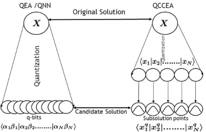
Typical EAs represent a candidate solution as a single point whereas QEA and QNN quantify the candidate solution as a linear combination of two components as shown in Fig.2-1. As the beneﬁt, the probability of reaching the optimal solution increases, and the convergence process to the optimal solution speeds up.

(13)

Figure 2-1: qubit (QEA) Vs subsolution points (QCCEA)

2.3 Quantum inspired Artiﬁcial Bee Colony

Algo-rithm (QABC)

Similar to QNN, QABC is also a QEA based algorithm developed by implementing quantum principles on artiﬁcial bee colony paradigm [33]. In QABC, individual is represented as a quantum vector (qubit) (similar to QEA). QABC algorithm is exe-cuted in 5 stages as detailed below. After initializing with a set of population, each individual qubit is projected in binary space by applying measurement operator and ﬁtness is calculated using

fiti =    1 1+fi if fi ≥0 1 + abs(fi) if fi <0 (2.4)

wherefirepresents the quality value of considered solution. This is followed by greedy

selection where the solution with the best fitness will remain. For exploring the search space QABC operator is used which is a quantified version of Artificial Bee Colony

(14)

operator which is deﬁned as vij   αij βij  =Xij   αij βij  +ϕij  Xij   αij βij  ₋Xik   αij βij     (2.5)

whereXi,Vi are discontinued and resultant solutions andXk is randomly selected

solution, D denotes the dimension of the problem and 1≤j ≤D, where j is the index chosen from the dimension and ϕij is a random number within the range [−1,1].

Population divergence is achieved by shifting qubit using quantum inheritance operator. For a qubit A(αA, βA) the resultant diversiﬁed qubit is calculated as αB =

best(i)+L∗αA

L+1 and βB =

√ 1−α2

B,where L is an integer coeﬃcient and best is the best

solution to be achieved. Whenbest(i) is guided to 1 , value ofα increases with which the probability of reaching 1 is reached and similar procedure is followed by guiding

best(i) to 0 which gives the value of β. QABC was evaluated on three numerical optimization functions Sphere, Rosenbrock and Griewank functions against quantum swarm algorithm and evolutionary algorithm and QABC outperforms both.

Inspired by the above quantum discipline that a candidate solution can be quan-tified as a set of subsolution points, I address CCEA and propose QCCEA whose candidate solutions are quantified into a non-linear combination of a fixed number of subsolution points. Fig. 2-1 gives an illustration of the proposed Quantization using subsolution points with a comparison to the traditional qubit quantization.

(15)

Chapter 3 Quantum Inspired Competitive

Coevolution (QCCEA)

3.1 Competitive Coevolution Algorithm (CCEA)

Competitive coevolution is the competitive approach of Darwins principle of survival of the fittest where individuals compete with each other resulting in a better species [34] [35]. In literature, three methods of competitive coevolution are prominent for selection of the most fit individuals [36], fitness sharing, shared sampling, and Hall of Fame (HF). In fitness sharing, every individual has a fitness sharing function which enables grouping other individuals with the similar fitness values [37]. This helps in identifying the most or least fit individuals in the population. Shared sampling is implemented only for small population sizes where individuals do not compete with the entire population, rather compete with only a sample taken from the population. In HF, each individual competes with every other individual in the population. In the beginning, the individuals compete with each other and the most fit individuals form a separate list called Hall of Fame (HF). In further generations the individuals compete with HF as well for the survival. HF gets updated as the generation progresses, thus forming a list of fit individuals for each generation.

(16)

Algorithm 1 Competitive coevolution algorithm 1: InitializeP1, ..., PM 2: repeat 3: fori= 1 toM do 4: xi= Select (Pm) 5: forj = 1 toM do 6: yi = Select(Pm) 7: if i <> jthen 8: X⇐Evaluate(xi, yj) 9: end if 10: end for

11: Evaluate (X,HF) /*Compete with Hall of Fame*/ 12: Update HF

13: end for

14: untilenough solutions are evaluated

tor for that generation. The fitness of every individual species in the population is evaluated againstxi (step 5). Resultant fit individual xis evaluated against HF. The individuals with better fitness are added into HF for competing with further gener-ations (Step 9). This process continues until enough solutions are evaluated. The fitness function of the individual xi is computed as

∑j i=1

(xs

i+ntime(xi)

j where ntime

is the number of generations since the individual is engaged in competition. New population is generated from the evaluated individuals.

There is a continuous diversity in the results since results depends on number of generations and time for each generation due to which the time period for reaching required solution is not deterministic. Another interesting aspect is that, since the selection is random, there is always a possibility of having required solution next to worst solution. When a worst possible solution is selected by random, the evolution process continues and time-frame for reaching the required solution cannot be guar-anteed. However there will be signiﬁcant improvement in quality of the solution with each generation [35].

(17)

3.2 Quantum Inspired Competitive Coevolution

(QC-CEA)

The essence of QCCEA is that, it disseminates the candidate solution into a collection of solution points. This is in the same discipline of QEA that enlarges the search space and refines optimization process by quantum bit implementation [7] [13]. Here, each solution point functions similar to that of a qubit in QEA to extend the search capability of CCEA. From one generation to another, more genetically diverse solution points (i.e., the normal distributions) are updated; that is the probabilities are refined such that the overall probability of finding the global optimal solution is increased and thus QCCEA is expected to be more resilient than CCEA towards the premature convergence problem.

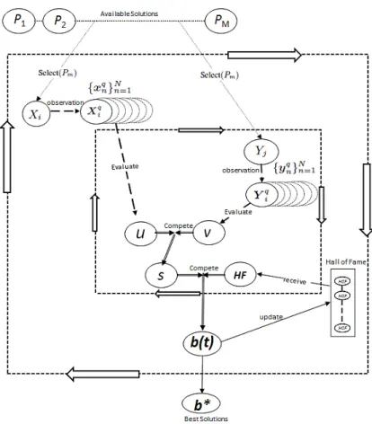
Figure 3-1: Overall structure of QCCEA

(18)

the population and is quantized followed by ﬁtness evaluation. This solution competes with all other solutions in the population. The winner among these two solutions will compete with HF resulting in the best solution b(t) for that cycle (represented in dotted interior square in Fig:3-1). HF is updated for each generation with the b(t) which is the best solution for that generation. The next solution is considered for competitions and this process (shown as dotted exterior square in Fig:3-1) continues till enough solutions are evaluated. Similar to CCEA new population is evolved with the combination of population in HF.

Algorithm 2 QCCEA: Quantum inspired Competitive coevolution (M, N, n, b∗) 1: InitializeP1, ..., PM; /*M solutions*/

2: Initialize b(1); /*current best solutions*/ 3: t←1; 4: HF(1)←P(1); 5: repeat 6: fori= 1 toM do 7: Xi= Select(Pm),1≤m≤M; 8: Quantize Xi = {xn}Nn=1 to X q

i = {xqn}Nn=1; /*constant variable xn is quantiﬁed as a

normal distribution vectorxq n*/ 9: fork= 1 toN do 10: u←u+ Evaluate (xk); 11: end for 12: forj= 1 toM andj ̸=ido 13: Yj= Select(Pm) ; 14: QuantizeYj ={yn}Nn=1 to Y q i ={y q n}Nn=1; 15: fork= 1 toN do 16: v←v+ Evaluate (yk); 17: end for 18: s⇐Max(Evaluate(u), Evaluate(v));

19: b(t)←max(Evaluate(s), Evaluate(HF(t))) /*Compute the best solution with current Hall of Fame*/

20: end for

21: Addb(t) intoHF(t); 22: end for

23: t←t+ 1;

24: b∗←maxEvaluate(HF(t)); /*select the best solution from current Hall of Fame*/ 25: untilenough solutions are evaluated

The QCCEA algorithm is detailed as Algorithm:2 and the procedure is described as follows.

QCCEA is initialized with a population of candidate solutions P1, P2, ..., PM

(step 1) whereM is the size of the population. HF and best solution of the generation

(19)

Xi = {xn}Nn=1, where m,i represent an individual from the population P of size M

and N represents the width of the search space. Quantifying Xi to Xqi = {xqn}Nn=1

wherexq

n is a normal distribution vector deﬁned asxqn = _σ√1₂_πe−

(x−µ)2

2σ2 . Each solution

point xq_k represents the kth _{part of} _Xq

i and is evaluated which constitutes u (step

10).SimilarlyYj is quantiﬁed asYqi and evaluated at component level, thus obtaining v (step 16).

As shown in Fig:3-1, quantified candidate solutionsuandvengages in competition (similar to CCEA) resulting insas the solution with best fitness amonguandv (step 18 of Algorithm:2). The competition betweensand the HF results in b, best solution for that generation (step 19). HF is always updated with b to maintain the most fit solution for that generation. This process continues till the exit criteria is met. The solution b∗ with maximum fitness among the available solutions of HF will be the best among all candidate solutions of the population.

(20)

Chapter 4 Experiments

4.1 Experimental Setup

Twenty benchmark functions [38] were used in this experimental studies. All functions are minimization problems deﬁned as:

M inf(x), x= [x1, x2, ..., xD], (4.1)

where D is the dimensionality of x. According to [39] [40] [41] , twenty benchmark functions is a suﬃcient number of functions to ﬁnd out whether the proposed QCCEA is better (or worse) than CCEA, and why. More multimodal functions are used since the local minima increases exponentially with the dimension [42] [43] resulting in increase of complexity which is an ideal challenge for many optimization algorithm evaluations.

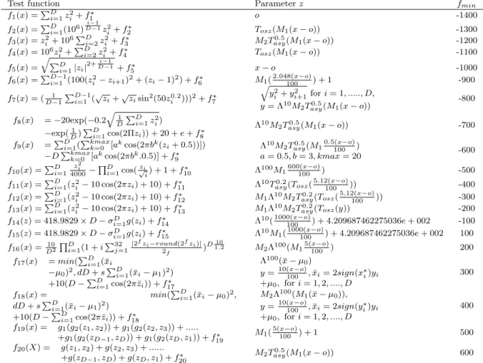
The mathematical description of the used functions is listed in Table 4.1, where functionsf1-f5 are unimodal functions andf6-f20 are basic multimodal functions.The detailed description of test functionsf19 and f20 is given in the Appendix A. In the table 4.1, M1, M2, ..., M10 are orthogonal (rotation) matrices generated from

stan-dard normally distributed entries by Gram-Schmidt ortho normalization which is a common practice for numerical optimization and o= [o1, o2, ..., oD] are the shifted

(21)

are shifted to o and scalable. Λα _{is a diagonal matrix in D dimensions with the} _ith diagonal element as λii=α i−1 2(D−1)_{, i}_{= 1}_,₂_{, ..., D.} Tβ asy : if xi >0, xi =x 1+β_Di−₋1₁√xi i ,for i= 1, ..., D

Tosz : for xi =sign(xi)exp(¯xi+ 0.049(sin(c1x¯i) +sin(c2x¯i))),for i= 1 andD

where ¯xi =    log(|xi|) if xi ̸= 0 0 otherwise , sign(xi) =          −1 if xi <0 0 if xi = 0 1 otherwise c1 =    10 if xi >0 5.5 otherwise ,and c2 =    7.9 if xi >0 3.1 otherwise

Table 4.1: BENCHMARK FUNCTIONS

Test function Parameterz fmin

f1(x) =∑Di=1zi2+f1∗ o -1400 f2(x) =∑Di=1(106) i−1 D−1_z2 i +f2∗ Tosz(M1(x−o)) -1300 f3(x) =zi2+ 106 ∑D i=2z2i+f3∗ M2Tasy0.5(M1(x−o)) -1200 f4(x) = 106zi2+ ∑D i=2zi2+f4∗ Tosz(M1(x−o)) -1100 f5(x) =√∑Di=1|zi|2+ i−1 D−1 ₊_f∗ 5 x−o -1000 f6(x) =∑_i=1D−1(100(z2i−zi+1)2+ (zi−1)2) +f6∗ M1(2.048(x₁₀₀−o)) + 1 -900 f7(x) = (_D1₋₁∑D_i=1−1(√zi+√zisin2(50zi0.2)))2+f7∗ √ y2 i +y2i+1fori= 1, ..., D, y= Λ10_M 2Tasy0.5(M1(x−o)) -800 f8(x) =−20exp(−0.2 √ 1 D ∑D i=1z2i) −exp(1 D) ∑D i=1cos(2Πzi)) + 20 +e+f8∗ Λ10_M 2Tasy0.5(M1(x−o)) -700 f9(x) =∑Di=1( ∑kmax k=0 [akcos(2πbk(zi+ 0.5))]) −D∑kmax_k=0 [ak_cos(2_πbk_.₀_._{5)] +}_f∗ 9 Λ10_M 2Tasy0.5(M10.5(x₁₀₀−o)) a= 0.5, b= 3, kmax= 20 -600 f10(x) =∑Di=1 z2 i 4000− ∏D i=1cos( zi √ i) + 1 +f10∗ Λ100M1600(x₁₀₀−o)) -500

f11(x) =∑Di=1(z2i−10 cos(2πzi) + 10) +f11∗ Λ10Tasy0.2(Tosz(5.12(x₁₀₀−o))) -400

f12(x) =∑Di=1(z2i−10 cos(2πzi) + 10) +f12∗ M1Λ10M2Tasy0.2(Tosz(5.12(x₁₀₀−o))) -300

f13(x) =∑Di=1(z2i−10 cos(2πzi) + 10) +f13∗ M1Λ10M2Tasy0.2(Tosz(y)) -200

f14(z) = 418.9829×D−σi=1D g(zi) +f14∗ Λ10( 1000(x−o) 100 ) + 4.209687462275036e+ 002 -100 f15(z) = 418.9829×D−σ_i=1D g(zi) +f15∗ Λ10M1( 1000(x−o) 100 ) + 4.209687462275036e+ 002 100 f16(x) = _D102 ∏D i=1(1 +i ∑32 j=1| 2f_z i−round(2fzi)| 2f ) D10 1.2 M2Λ100(M15(x₁₀₀−o)) 200 f17(x) =min(∑Di=1(¯xi −µ0)2, dD+s∑_i=1D (¯xi−µ1)2) +10(D−∑D_i=1cos(2πz¯i)) +f17∗ Λ100_(¯_x₋_µ 0) y= 10(x₁₀₀−o),x¯i= 2sign(x∗i)yi +µ0, fori= 1,2, ...., D 300 f18(x) = min(∑i=1D (¯xi−µ0)2, dD+s∑Di=1(¯xi−µ1)2) +10(D−∑D_i=1cos(2πz¯i)) +f18∗ M2Λ100(M1(¯x−µ0)), y= 10(x₁₀₀−o),x¯i= 2sign(y∗i)yi +µ0, fori= 1,2, ...., D 400 f19(x) = g1(g2(z1, z2)) +g1(g2(z2, z3)) +... +g1(g2(zD−1, zD)) +g1(g2(zD, z1)) +f₁₉∗ M1( 5(x−o) 100 ) + 1 500 f20(X) = g(z1, z2) +g(z2, z3) +... +g(zD−1, zD) +g(zD, z1) +f20∗ M2Tasy0.5(M1(x−o)) 600

For all experiments, same population size (100), same search range and same dimension is used. Same initial population is maintained for both CCEA and QCCEA. For simplicity, all the test functions are set with the same search range as [−100,100]D_.

(22)

3000 generations and each algorithm is executed 25 times.

4.2 Unimodal Funtions

The ﬁrst set of experiments are on functions f1−f5. The obtained average results of 25 runs evolutions are presented in Table 4.2.

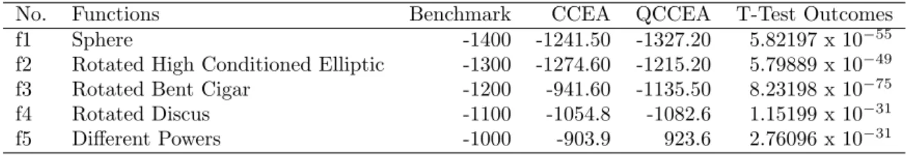
Table 4.2: CCEA Vs QCCEA ON UNIMODAL FUNCTIONSf1−f5

No. Functions Benchmark CCEA QCCEA T-Test Outcomes f1 Sphere -1400 -1241.50 -1327.20 5.82197 x 10−55

f2 Rotated High Conditioned Elliptic -1300 -1274.60 -1215.20 5.79889 x 10−49

f3 Rotated Bent Cigar -1200 -941.60 -1135.50 8.23198 x 10−75 f4 Rotated Discus -1100 -1054.8 -1082.6 1.15199 x 10−31 f5 Diﬀerent Powers -1000 -903.9 923.6 2.76096 x 10−31

4.3 Multimodal Functions

The second set of experiments are aimed at 15 basic multimodal functions f6-f20. Multimodal functions are often regarded diﬃcult to be optimized because of their multiple local minimum values exists in a huge local optima search space [39]. The global optima of functions f11-f15 is far from their local optima, whereas function

f6 has a narrow valley between its local and global optima. Functions f16 and f18 are extremely diﬃcult to be optimized since their local minimum values are present everywhere inside the search space and are non diﬀerentiable.

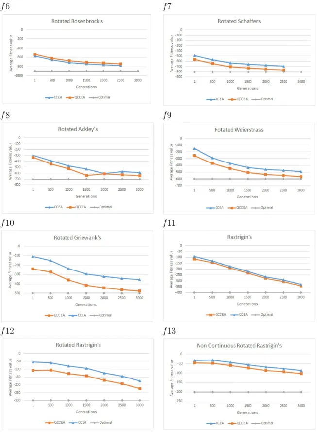
Table 4.3 summarizes the average ﬁtness values obtained when applying proposed QCCEA to optimize the considered functions. It contains also the average ﬁtness val-ues of CCEA for comparison. Fig.5-2 and Fig. 5-3 shows the progressive convergence of all multimodal functions.

(23)

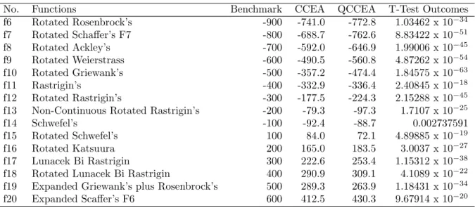
Table 4.3: CCEA Vs QCCEA ON MULTIMODAL FUNCTIONSf6−f20

No. Functions Benchmark CCEA QCCEA T-Test Outcomes f6 Rotated Rosenbrock’s -900 -741.0 -772.8 1.03462 x 10−34 f7 Rotated Schaﬀer’s F7 -800 -688.7 -762.6 8.83422 x 10−51 f8 Rotated Ackley’s -700 -592.0 -646.9 1.99006 x 10−45 f9 Rotated Weierstrass -600 -490.5 -560.8 4.87262 x 10−54 f10 Rotated Griewank’s -500 -357.2 -474.4 1.84575 x 10−63 f11 Rastrigin’s -400 -332.9 -336.4 2.40845 x 10−18 f12 Rotated Rastrigin’s -300 -177.5 -224.3 2.15288 x 10−45

f13 Non-Continuous Rotated Rastrigin’s -200 -79.3 -97.3 1.7107 x 10−25

f14 Schwefel’s -100 -92.4 -88.7 0.002737591 f15 Rotated Schwefel’s 100 84.0 72.1 4.89885 x 10−19

f16 Rotated Katsuura 200 165.0 183.5 3.0037 x 10−27

f17 Lunacek Bi Rastrigin 300 222.6 253.4 1.15312 x 10−38 f18 Rotated Lunacek Bi Rastrigin 400 290.9 309.1 4.1089 x 10−22 f19 Expanded Griewank’s plus Rosenbrock’s 500 289.3 263.9 1.18431 x 10−34 f20 Expanded Scaﬀer’s F6 600 412.5 430.3 9.67914 x 10−20

(24)

Chapter 5 Discussion

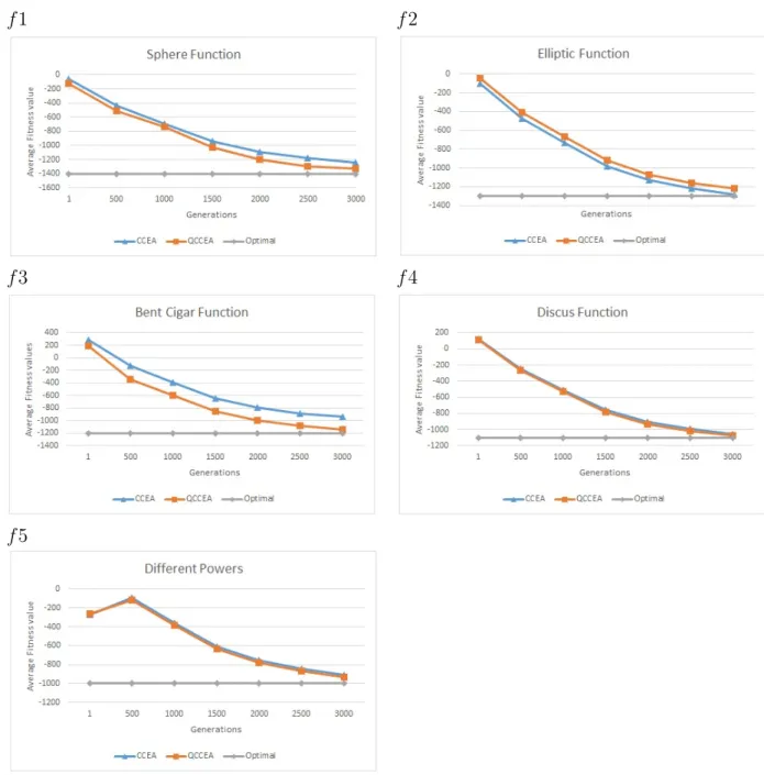
Fig.5-1 shows respectively the progress of average fitness of CCEA and QCCEA for the five test functions over 25 runs. As seen from the results, QCCEA performs consistently closer to the optimum or near optimum than CCEA for four of total five unimodal functions. For function f2, QCCEA lags behind CCEA with a statistically negligible difference of 4.8%.

Sphere Function f1 is a commonly used initial test function for performance eval-uation of numerical optimization algorithms. For function f1 both CCEA and QC-CEA exhibited similar performance at the beginning (till 721 generations) but at the later stages, QCCEA has improved progressively due to quantization. QCCEA has dominated in 2279 generations out of 3000 for function f1.

The biggest performance superiority of QCCEA occurs with Rotated Bent Cigar functionf3 which is 17%. QCCEA achieved better convergence rate than CCEA due to its extensive search ability for the same number of generations while CCEA was caught within a small search space.

As shown in Table 4.3, QCCEA outperforms CCEA for twelve out of ﬁfteen func-tions. Moreover, QCCEA performed equally well for two out of three CCEA domi-nated functions. The highest performance dominance of QCCEA over CCEA is 24% , which occurs with f10, the Rotated Griewank’s function as shown in Fig. 5-2 .

For Rotated Ackley’s function f8 shown in Fig.5-2, QCCEA reaches the best ﬁtness (at generation 1500) 500 generations faster than CCEA. Interestingly, both

(25)

f1 f2

f3 f4

f5

(26)

f6 f7

f8 f9

f10 f11

f12 f13

(27)

f14 f15

f16 f17

f18 f19

f20

(28)

QCCEA and CCEA reaches the same ﬁtness value at generation 2000, but QCCEA wins over CCEA for rest of the generations. Both the algorithms are unable to retain their search boundaries to the near optimal value since functionf8 is an asymmetrical function.

For Rotated Rastrigin’s function f12, both algorithms could not even reach near optimal value as shown in Fig.5-2. Nevertheless, QCCEA’s performance is outstand-ing. In this, QCCEA reaches 25% away from the optima, which is 20% closer to the optima than the CCEA.

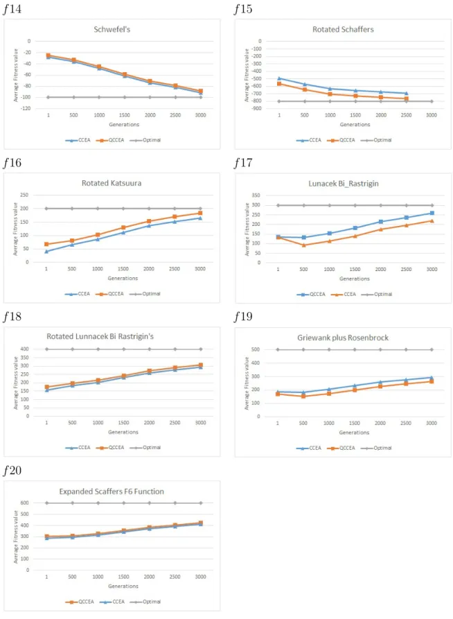
For Lunacek Bi Rastrigin function f17, both QCCEA and CCEA starts at the same point, but the performance of CCEA declines within the ﬁrst 500 generations and maintains the same convergence rate for the remaining 2500 generations as ob-served in Fig.5-3. In contrast, QCCEA forms average 12.1% superiority to CCEA during the ﬁrst 500 generations, and this superiority is retained until the last gener-ation.

From the above analysis, it is evident that QCCEA has a controlled performance irrespective of shape, properties and local minimum implications of the functions whereas CCEA was unable to adjust itself accordingly. For rest of the QCCEA domi-nated functions, the progressive convergence of QCCEA against CCEA is consistent. For the three functions f14,f15 and f19 where QCCEA fall short of CCEA, the diﬀerence in the average ﬁtness is 1%, 10.6% and 7.5% respectively, as represented in Fig.5-3

(29)

Chapter 6 Conclusion

This thesis presented QCCEA, a new quantum inspired competitive coevolution al-gorithm. In QCCEA, candidate solution is represented through a combination of a set of solution points which are jointly described through normal distributions. This is different from traditional quantization methods such as QEA [7] and QNN [13]. The performance of the proposed QCCEA is evaluated on 20 benchmark numerical optimization functions published in CEC 2013 [38]. According to the obtained exper-iment results, QCCEA is outperforming CCEA over 16 out of 20 test functions, and the search speed of the QCCEA is noticeably faster in that QCCEA reaches global optima or near optima in less number of generations than that of CCEA. Statistical study based on the obtained results also shows that QCCEA can maintain a good balance between exploitation and exploration over the whole search space. It is there-fore more effective in identifying global optimal solutions. Based on these findings, it can be finally concluded that quantum computing principles developed in this paper can help to improve the performance of coevolutionary algorithms.

QCCEA, as presented in this paper, is only suitable for tackling numerical opti-mization problems. Looking into the future, it remains interesting to see how QCCEA can be further extended in order to solve combinatorial optimization problems that are of particular interests in practical applications. It is also interesting to extensively evaluate the potential and eﬀectiveness of QCCEA for general-purpose machine learn-ing and decision maklearn-ing tasks.

(30)

Appendix A

Test Functions

f

19 and

f

20

A.1 f

19 Expanded Griewanks plus Rosenbrocks

Func-tion

Griewank’s Function g1(x) = ∑D i=1 x2 i 4000 − ∏D i=1cos( xi √ i) + 1 Rosenbrock’s Function g2(x) = ∑D−1 i=1 (100(x 2 i −xi+1)2+ (xi−1)2) f19(x) =g1(g2(z1, z2)) +g1(g2(z2, z3)) +...+g1(g2(zD−1, zD)) +g1(g2(zD, z1)) +f19∗ z =M1( 5(x−o) 100 ) + 1

A.2 f

20 Expanded Scaﬀers F6 Function

g(x, y) = 0.5 + (sin2( √ x2₊_y2₎₋₀_.₅₎ (1+0.001(x2₊_y2₎₎ , f20(X) =g(z1, z2) +g(z2, z3) +...+g(zD−1, zD) +g(zD, z1) +f20∗ z =M2Tasy0.5(M1(x−o))

(31)

Bibliography

[1] F. J. Gomez and R. Miikkulainen, “Solving non-markovian control tasks with neuroevolution,” in Proceedings of the 16th international joint conference on Artificial intelligence - Volume 2, IJCAI’99, pp. 1356–1361, 1999.

[2] C. Young and R. Miikkulainen, “Cooperative coevolution of multi-agent sys-tems,” Autonomous Mental Development, pp. A101–287, 2001.

[3] C. Young and R. Miikkulainen, “Coevolution of role-based cooperation in mul-tiagent systems,” Autonomous Mental Development, pp. 170–186, 2009.

[4] L. Panait, S. Luke, and R. P. Wiegand, “Biasing coevolutionary search for op-timal multiagent behavior,” IEEE Transactions on Evolutionary Computation, vol. 10, no. 6, pp. 629 – 645, 2006.

[5] K. O. Stanley and R. Miikkulainen, “Evolving a roving eye for go,” in Proceed-ings of the Genetic and Evolutionary Computation Conference (GECCO-2004), (Berlin), Springer Verlag, 2004.

[6] K.-H. Han and J. hwan Kim, “Quantum-inspired evolutionary algorithm for a class of combinatorial optimization,” IEEE TRANS. EVOLUTIONARY COM-PUTATION, vol. 6, pp. 580–593, 2002.

[7] K. H. Han, Quantum-inspired Evolutionary Algorithm. PhD thesis, Korea Ad-vanced Institute of Science and Technology KAIST, 2003.

[8] J.-S. Jang, “Face detection using quantum-inspired evolutionary algorithm,” in

in Proc. IEEE Congress on Evolutionary Computation, pp. 2100–2106, 2004. [9] J.-S. Jang, K.-H. Han, and J.-H. Kim, “Quantum-inspired evolutionary

algorithm-based face veriﬁcation,” in Proceedings of the 2003 international con-ference on Genetic and evolutionary computation: PartII, GECCO’03, (Berlin, Heidelberg), pp. 2147–2156, Springer-Verlag, 2003.

[10] M. D. Platel, S. Schliebs, and N. Kasabov, “Quantum-inspired evolutionary al-gorithm: a multimodel eda,” Trans. Evol. Comp, vol. 13, pp. 1218–1232, Dec. 2009.

(32)

[11] K.-H. Han and J.-H. Kim, “Quantum-inspired evolutionary algorithms with a new termination criterion, h gate, and two-phase scheme,” Trans. Evol. Comp, vol. 8, pp. 156–169, Apr. 2004.

[12] R. Hinterding, “Representation, constraint satisfaction and the knapsack prob-lem,” in Evolutionary Computation, 1999. CEC 99. Proceedings of the 1999 Congress on, vol. 2, pp. –1292 Vol. 2, 1999.

[13] T.-C. Lu, G.-R. Yu, and J.-C. Juang, “Quantum-based algorithm for optimiz-ing artiﬁcial neural networks,” Neural Networks and Learning Systems, IEEE Transactions on, vol. 24, no. 8, pp. 1266–1278, 2013.

[14] J. S. Bell, “On the Problem of Hidden Variables in Quantum Mechanics,”

Rev.Mod.Phys., vol. 38, pp. 447–452, 1966.

[15] C. Xu, L. liang Yang, R. Maunder, and L. Hanzo, “Near-optimum soft-output ant-colony-optimization based multiuser detection for the ds-cdma uplink,” 2009. [16] R. Feynman and P. W. Shor, “Simulating physics with computers,” SIAM

Jour-nal on Computing, vol. 26, pp. 1484–1509, 1982.

[17] P. Benioﬀ, “Quantum mechanical hamiltonian models of turing machines,” Jour-nal of Statistical Physics, vol. 29, no. 3, pp. 515–546, 1982.

[18] T. Hey, “Quantum computing: an introduction,” Computing Control Engineer-ing Journal, vol. 10, no. 3, pp. 105–112, 1999.

[19] H. Wimmel, Quantum Physics and Observed Reality:A Critical Interpretation of Quantum Mechanics. World Scientiﬁc Pub Co Inc, 1992.

[20] D. Deutsch, “Quantum theory the church-turing principle and the universal quantum computer,” ” ”, pp. 97–117, 1985.

[21] D. Deutsch and R. Jozsa, “Rapid solution of problems by quantum computation,”

Proceedings of the Royal Society of London Series A, vol. 439, pp. 553–558, 1992. [22] P. W. Shor, “Algorithms for quantum computation: Discrete logarithms and fac-toring,” in SFCS ’94 Proceedings of the 35th Annual Symposium on Foundations of Computer Science, pp. 124–134, 1994.

[23] R. Cleve, A. Ekert, C. Macchiavello, and M. Mosca, “Quantum algorithms re-visited,” in Proceedings of the Royal Society of London A, pp. 339–354, IEEE Computer Society, 1998.

[24] L. K. Grover, “A fast quantum mechanical algorithm for database search,” in

ANNUAL ACM SYMPOSIUM ON THEORY OF COMPUTING, pp. 212–219,

ACM, 1996.

[25] L. K. Grover, “Quantum mechanical searching,” in Congress on Evolutionary Computation, pp. 2255–2261, IEEE Press, 1999.

(33)

[26] F. Li, M. Zhou, and H. Li, “A novel neural network optimized by quantum genetic algorithm for signal detection in mimo-ofdm systems,” in Computational Intelli-gence in Control and Automation (CICA), 2011 IEEE Symposium on, pp. 170– 177, 2011.

[27] Y. Wang, X.-Y. Feng, Y.-X. Huang, D.-B. Pu, W.-G. Zhou, Y.-C. Liang, and C.-G. Zhou, “A novel quantum swarm evolutionary algorithm and its applications,”

Neurocomputing, vol. 70, no. 46, pp. 633 – 640, 2007.

[28] A. Narayanan and M. Moore, “Quantum-inspired genetic algorithms,” in In Proceedings of the 1996 IEE InternationalConference on Evolutionary Computa-tion(ICEC96, pp. 61–66, Press, 1995.

[29] F. Li, L. Hong, and B. Zheng, “Quantum genetic algorithm and its application to multi-user detection,” in Signal Processing, 2008. ICSP 2008. 9th International Conference on, pp. 1951–1954, 2008.

[30] K. H. Han and J. H. Kim, “Genetic quantum algorithm and its application to combinatorial optimization problem,” in Evolutionary Computation, 2000. Proceedings of the 2000 Congress on, vol. 2, pp. 1354–1360 vol.2, 2000.

[31] K.-H. Han, K. hong Park, C. ho Lee, and J. hwan Kim, “Parallel quantum-inspired genetic algorithm for combinatorial optimization problem,” in in Proc. 2001 Congress on Evolutionary Computation. Piscataway, NJ: IEEE, pp. 1422– 1429, Press, 2001.

[32] Y. Kim, J.-H. Kim, and K.-H. Han, “Quantum-inspired multiobjective evolu-tionary algorithm for multiobjective 0/1 knapsack problems,” in Evolutionary Computation, 2006. CEC 2006. IEEE Congress on, pp. 2601–2606, 2006. [33] A. Bouaziz, A. Draa, and S. Chikhi, “A quantum-inspired artiﬁcial bee colony

algorithm for numerical optimisation,” in Programming and Systems (ISPS), 2013 11th International Symposium on, pp. 81–88, April 2013.

[34] C. Darwin,On the Origin of the Species by Means of Natural Selection: Or, The Preservation of Favoured Races in the Struggle for Life, pp. 1–502. John Murray, 1859.

[35] K. O. Stanley and R. Miikkulainen, “Competitive coevolution through evolu-tionary complexiﬁcation,” Journal of Artificial Intelligence Research, vol. 21, pp. 63–100, 2004.

[36] C. D. Rosin and R. K. Belew, “New methods for competitive coevolution,” Jour-nal Evolutionary Computation, vol. 5, pp. 1–29, Mar. 1997.

[37] P. J. Angeline and J. B. Pollack, “Competitive environments evolve better so-lutions for complex tasks,” in Fifth International Conference on Genetic Algo-rithms, ICGA, 1993.

(34)

[38] J. Liang, B. Qu, P. N. Suganthan, and A. G. Hernndez-Daz, “Problem deﬁni-tions and evaluation criteria for the cec 2013 special session on real-parameter optimization,” tech. rep., Nanyang Technological University, 2013.

[39] X. Yao, Y. Liu, and G. Lin, “Evolutionary programming made faster,” Evolu-tionary Computation, IEEE Transactions on, vol. 3, no. 2, pp. 82–102, 1999. [40] D. Wolpert and W. Macready, “No free lunch theorems for optimization,”

Evo-lutionary Computation, IEEE Transactions on, vol. 1, no. 1, pp. 67–82, 1997. [41] D. H. Wolpert and W. G. Macready, “No free lunch theorems for search,” 1995. [42] A. A. Trn and A. Zilinskas, Global Optimization, vol. 350 of Lecture Notes in

Computer Science. Springer, 1989.

[43] H.-P. P. Schwefel, Evolution and Optimum Seeking: The Sixth Generation. New York, NY, USA: John Wiley & Sons, Inc., 1993.

A quantum inspired competitive coevolution evolutionary algorithm