Author’s Accepted Manuscript
Trajectory Tracking Passivity-based Control for
Marine Vehicles Subject to Disturbances
Alejandro Donaire, Jose Guadalupe Romero,
Tristan Perez
PII:
S0016-0032(17)30023-6
DOI:
http://dx.doi.org/10.1016/j.jfranklin.2017.01.012
Reference:
FI2868
To appear in:
Journal of the Franklin Institute
Received date: 4 May 2016
Revised date:
18 November 2016
Accepted date: 11 January 2017
Cite this article as: Alejandro Donaire, Jose Guadalupe Romero and Tristan
Perez, Trajectory Tracking Passivity-based Control for Marine Vehicles Subject
to
Disturbances,
Journal
of
the
Franklin
Institute,
http://dx.doi.org/10.1016/j.jfranklin.2017.01.012
This is a PDF file of an unedited manuscript that has been accepted for
publication. As a service to our customers we are providing this early version of
the manuscript. The manuscript will undergo copyediting, typesetting, and
review of the resulting galley proof before it is published in its final citable form.
Please note that during the production process errors may be discovered which
could affect the content, and all legal disclaimers that apply to the journal pertain.
Trajectory Tracking Passivity-based Control for Marine Vehicles
Subject to Disturbances
Alejandro Donairea,b,∗, Jose Guadalupe Romeroc, Tristan Perezd
aPRISMA Lab, Department of Electrical Engineering and Information Technology, University of Naples
Federico II, Italy
bSchool of Engineering, The University of Newcastle, Australia
cDepartamento Acad´emico de Sistemas Digitales, Instituto Tecnol´ogico Aut´onomo de M´exico-ITAM, Rio
Hondo No.1, 01080, Distrito Federal, M´exico.
dInstitute for Future Environments and School of Electrical Eng. and Comp. Sc., Queensland University of
Technology, Australia
Abstract
In this paper we present a dynamic model of marine vehicles in both body-fixed and inertial momentum coordinates using port-Hamiltonian framework. The dynamics in body-fixed coordinates have a particular structure of the mass matrix that allows the application of passivity-based control design developed for robust energy shaping stabilisation of mechani-cal systems described in terms of generalised coordinates. As an example of application, we follow this methodology to design a passivity-based controller with integral action for fully actuated vehicles in six degrees of freedom that tracks time-varying references and rejects disturbances. We illustrate the performance of this controller in a simulation example of an open-frame unmanned underwater vehicle subject to both constant and time-varying dis-turbances. We also describe a momentum transformation that allows an alternative model representation of marine craft dynamics that resembles general port-Hamiltonian mechanical systems with a coordinate dependent mass matrix.
Keywords: Marine robotics, Port-Hamiltonian Systems, Integral Control, Disturbance Rejection.
1. Introduction
Interconnection and damping assignment passivity-based control (IDA-PBC) is an at-tractive technique for designing motion-control strategies for physical dynamic systems. This technique uses the control action to transform the open-loop system into a closed-loop sys-tem in port-Hamiltonian (pH) form [1, 2]. The closed-loop potential energy is chosen such that it attains its minimum at the desired configuration of the system—this determines
∗Corresponding author
Email addresses: [email protected](Alejandro Donaire),
the closed-loop equilibrium. Under certain conditions on different terms of the closed-loop model, stability can be proven using the closed-loop energy as a Lyapunov function. The design also exhibits passivity properties with respect to force inputs and velocity outputs.
The passivity properties of the hydrodynamic and rigid-body models of marine craft have been exploited for design of motion control systems. For example, in [3] (see also the summary in [4]), the authors use the concept of vectorial-integrator backstepping for the design of dynamic positioning for ships—a technique that uses control-Lyapunov functions and can be related to feedback passivation [5]. In [6], the authors use passivity-based tech-niques to design a ride controller (reduction of roll and pitch) for a surface-effect ship. In [7], the authors consider the dynamics of fully-actuated underwater vehicles as a Hamilto-nian system, and address the problem of stabilisation of underwater vehicles using internal rotors as actuators. This control approach involves shaping the kinetic energy of the vehicle preserving the Hamiltonian structure and adding dissipation to ensure asymptotic stability of the closed-loop. The use of IDA-PBC for positioning with integral action of open-frame fully-actuated underwater vehicles is addressed in [8] and this work is extended to track-ing in [9] in three degrees of freedom (DOF). Considerations of actuator saturation and the addition of remedial anti-windup is addressed in [10] for the problem of dynamic po-sitioning of offshore vessels. In [11], the authors consider the problem of stabilisation of the under-actuated Kirchhoff equations for an underwater vehicle moving in an ideal fluid, that is, neglecting hydrodynamic dissipative forces. The latter authors apply IDA-PBC to deal with the stabilisation problems of the steady longitudinal motion and the steady ris-ing/diving with forward/reverse motion. In [12], the authors solve the attitude and speed regulation problem for a slender underwater vehicle with a full hydrodynamic model (poten-tial plus viscous effects) and focus on both forward speed and attitude (roll, pitch, and yaw) tracking based on energy shaping and damping assignment such that the closed-loop system retains a port-Hamiltonian form. The unactuated channels of the system are left in open loop, and a suppression control is used to completely remove the uncontrolled behaviour from the target (closed-loop) dynamics.
In this paper, we present Hamiltonian models of marine vehicle dynamics in six DOF in both body-fixed and inertial momentum coordinates. The model in body-fixed coordinates exhibits a particular structure of the mass matrix that allows the adaptation and application of a change of coordinates to assign a full-rank dissipation matrix first proposed in [10], and then generalised for mechanical systems in [13, 14]. We follow this approach to design a passivity-based tracking controller with integral action for fully actuated vehicles in six DOF. This extends the work in [10] that only considers the set-point regulation problem in 3DOF to trajectory tracking in six DOF. The work in [9] consider the tracking problem, however, the proof only ensure asymptotically stability, and rejection of constant disturbance is not theoretically ensured. In this paper, we prove exponential stability of the tracking error as well as rejection of constant disturbances and bounded-input-bounded-state of the closed loop. In this paper we expand the development of the model and the numerical simulations performed in our preliminary work [15]. We also describe a momentum transformation that allows an alternative model representation that resembles general port-Hamiltonian mechanical systems with a coordinate dependent mass matrix. This similarities can be
exploited to adapt the theory of control of port-Hamiltonian systems developed in robotic manipulators and mechanical systems to the case of marine craft dynamics.
Notation. In this paper we use the following notation: we note the standard 2 norm of a
vectorv as |v|=√vTv, and its induced norm for a matrix A and |A|.
2. Port-Hamiltonian systems
2.1. Modelling
The dynamics of mechanical systems can be described using a a set of 2n first-order differential equations known as a Hamilton’s canonical equations of motion [16]:
˙
q=∇pH(p, q), (1)
˙
p=−∇qH(p, q) +τ, (2)
where q and p are the n-dimensional vectors of generalised coordinates and momenta re-spectively, and τ is the vector of generalised forces. The Hamiltonian H(p, q) is the sum of the kinetic energy and the potential energy:
H(p, q) = 1 2p
TM−1(q)p+V(q). (3)
This function represents the total energy of the system. The Hamilton equations (1)-(2) is a particular state-space representation of the system dynamics equivalent to the classi-cal Euler-Lagrange models. We should note, however, that there are systems that admit Hamiltonian but not Lagrangian representations [16].
In the control literature, the Hamiltonian model (1)-(2) has been generalised to what is known as a port-Hamiltonian system [17]:
˙
x = [Jo(x)−Ro(x)]∇H(x) +Go(x)u, (4)
y = GTo(x)∇H(x), (5)
wherexis the state vector and the pairu, y are the input and outputm-dimensional vectors. These are conjugate variables in the sense that their inner product represents (or is akin to) the power exchanged between the system and its environment. The functionJo(x) = −JoT(x)
describes the power preserving interconnection structure through which the components of the system exchange energy. The symmetric function Ro(x) ≥ 0 captures dissipative
phenomena in the system. The functionGo(x) weighs the action of the input on the system
and defines the conjugate output. From (4)-(5), it follows that ˙
H(x) = yTu−[∇H(x)]TRo(x)∇H(x)≤yTu, (6)
2.2. Interconnection and damping assignment passivity-based control
Following [18], consider the open-loop system of the form ˙
x=f(x) +g(x)u. (7)
The idea of IDA-PBC is to use the state-feedback control law u = K(x) to re-shape the system (7) into thedesired closed-loop system or target dynamics
˙
x= [Jd(x)−Rd(x)]∇Hd(x), (8)
whereJd(x) =−JdT(x),Rd(x)>0, and the desired Hamiltonian attains its minimum at the
desired equilibrium state:
x∗ = arg min
x Hd(x). (9)
The stability of the equilibrium x∗ can be established using Hd(x) as Lyapunov function.
Such design specifies the interconnection Jd, injects damping through the dissipation
functionRd, and shapes the system energy such that the minimum is at the equilibriumx∗.
A control law of the formu=K(x) exists provided that the following PDE can be solved:
g⊥(x)[f(x)−(Jd(x)−Rd(x))∇Hd(x)] = 0, (10)
whereg⊥(x) is the full-rank left annihilator of g(x). This leads to the general form
u=K(x) = [gT(x)g(x)]−1gT(x)[(Jd(x)−Rd(x))∇Hd(x)−f(x)]. (11)
If the control is for a fully-actuated open loop system, it is not necessary to solve the matching PDE (10) since one can propose the desired Hamiltonian and constructively determine the functionsJdandRd. This is the procedure we follow in Section 4 of this paper. The problem
of tracking is addressed in a similar fashion as described above, but the target dynamics is associated with the tracking error. This design requires not only the desired referencex∗(t) but also its time derivatives. For further details on IDA-PBC, see for example [2, 1, 19, 18].
3. Dynamics of marine craft in port-Hamiltonian form
The design of an IDA-PBC control strategy can be aided in some cases if the open-loop control system itself is described as a pH system. Such description exhibits energy properties of the open-loop system that a control design can exploit and seek to preserve. Therefore, in this section, we formulate the open-loop models of marine craft in pH form.
The classical equations of motion used for marine craft can be written as follows [20]: ˙
η=J(η)ν, (12)
Mν˙ +C(ν)ν+D(ν)ν+G(η) = τc+τd, (13)
whereηdescribe the pose of the vehicle (position and orientation) (North, East, Down, roll, pitch, yaw),ν is the body-fixed linear-angular velocity (surge, sway, heave, roll, pitch, yaw).
The vectorτc represents the force and torque control inputs (surge, sway, heave, roll, pitch,
yaw), and τd represent the force and torque disturbance inputs. The constant matrixM =
MT >0 is the total generalised mass matrix due to rigid-body mass distribution and fluid
added mass,C(ν) = −CT(ν) is the total Coriolis-centripetal matrix, and D(ν) = DT(ν)>0
is the total hydrodynamic damping matrix, andG(η) is the vector of hydrostatic forces and torques due to gravity and buoyancy. The functionJ(η) is a 6×6 kinematic transformation matrix, which is well-defined if the pitch angleθ 6=±π
2 (see e.g. [4] for details on this model).
Following on of the work in [10], we will write the dynamics (12)-(13) in pH form. We first make the following assumption:
Assumption 1 (A1). There exist a potential function V(η) :R3× S3 →
R that satisfies JT(η)∇ηV(η) =G(η). (14)
By Poincare’s Lemma, a necessary and sufficient condition for the existence of V(η) is that
∇η
J−T(η)G(η) = ∇η
J−T(η)G(η)T. (15) Note that this equation is satisfied for example by neutrally buoyant underwater vehicles. For the latter, the functionV has the form
V(η) = −Wsin(θ)X+Wcos(θ) sin(φ)Y +Wcos(θ) cos(φ)Z, (16) where W = mg is the submerged weigh of the vehicle, and (X, Y, Z) are the cartesian coordinates of the centre of buoyancy relative to the centre of gravity.
3.1. pH Model in Body-fixed Coordinates
The following proposition establishes the pH model in terms of a transformation of the body-fixed velocity.
Proposition 3.1. Consider the dynamics (12)-(13). Then under assumption A1, the
dy-namics of the marine craft can be written in port-Hamiltonian form as follows
˙ η ˙ p = 0 J(η) −JT(η) −J 2(p) ∇H+ 0 In (τc+τd), (17) where H(η, p) = 1 2p TM−1p+V(η), (18)
the momentum is defined through the following transformation of the body-fixed velocities1:
p=M ν, (19) and J2(p) = C(ν) +D(ν) ν=M−1p, which satisfiesJ2(p) +J T 2(p)>0.
1Note that the momentum (19) is not the conjugate momentum of the generalised coordinate vectorη
since ν has as components the body-fixed angular velocity (quasi-coordinates) [21, p193]. These do not
Proof The proof follows from construction of the state equations for η and p. First, we note that
˙
η = J(η)ν =J(η)M−1p
= J(η)∇pH, (20)
which is the first row of (17). Then, from (13) we obtain ˙ p = Mν˙ = −G(η)−C(ν)ν−D(ν)ν+τc+τd = −JT(η)∇ ηV(η)−J2(p)M−1p+τc+τd = −JT(η)∇ ηH−J2(p)∇pH+τc+τd, (21)
which is the second row of (17). The fact the J2(p) is positive definite follows readily from
the properties of C(ν) =−CT(ν) and D(ν) =DT(ν)>0.
3.2. pH Model in Inertial Coordinates
An alternative port-Hamiltonian model, still under assumption A1, can be built by defin-ing a new momentum vector as follows2
`=J−T(η)M ν. (22)
Then, usingη and ` as states, the marine craft dynamics (17) can be written as follows ˙ η ˙ ` = 0 In −In −L(η, `) ∇Hη + 0 J−T(η) (τc+τd), (23) where Hη(η, `) = 1 2` T J(η)M−1JT(η)`+V(η), (24) = 1 2` T Mη−1(η)`+V(η), (25) and L(η, `) = n X i=1 ∇ηi[J −T ]M νeTi !T − n X i=1 ∇ηi[J −T ]M νeTi + +J−TC(ν)J−1+J−TD(ν)J−1 ν=M−1JT` , (26)
2The matrixJ−1(η) is well-defined if the pitch angleθ6=±π
where ei ∈Rn is the i−th vector of the Euclidean orthonormal basis. The first three terms
of the matrix L(η, `) in (26) determine the skew-symmetric component of the matrix and accounts for the gyroscopic forces, whilst the last term describes the damping and implies that L(η, `) +LT(η, `) > 0. Note that the expression of Hamiltonian function (24) and
(25) are equivalent, but (24) uses a factorisation of the mass matrix in terms of J. This factorisation, which also arises from expressing the kinetic co-energy in terms of ˙η, inspires a change of momenta to obtain a pH model with constant mass matrix as in (17). This type of change of coordinates has also been used in the literature to obtain an identity mass matrix in body-fixed momentum coordinate and been exploited to design controllers and observers for general mechanical systems, see for example [13, 22].
The dynamics (23) is obtained in two steps. First, we notice that we can write ˙
η = J(η)ν=J(η)M−1JT(η)`
= Mη−1(η)`, (27)
which is the first row of (23). Second, we compute the derivative of (22) with respect to time as follows ˙ ` = d dt J−T(η)M ν = ˙J−T(η)p+J−T(η) ˙p = n X i=1 ∇ηi[J −T ]M νeTiη˙− ∇ηV −J−TJ2M−1JT`+J−T(τc+τd) = n X i=1 ∇ηi[J −T ]M νeTi∇`Hη− ∇ηV −J−TJ2M−1JT`+J−T(τc+τd) + " n X i=1 ∇ηi[J −T]M νeT i #T ∇`Hη− " n X i=1 ∇ηi[J −T]M νeT i #T ∇`Hη (28)
Then, using the fact that
−1 2∇η `TJ M−1JT` = " n X i=1 ∇ηi[J −T ]M νeTi #T ∇`Hη (29) in (28), we obtain ˙ ` = −1 2∇η `TJ M−1JT`− ∇ηV −J−TJ2J−1∇`Hη+J−T(τc+τd) + n X i=1 ∇ηi[J −T ]M νeTi∇`Hη − " n X i=1 ∇ηi[J −T ]M νeTi #T ∇`Hη = −∇ηHη − J−TJ2J−1− n X i=1 ∇ηi[J −T ]M νeTi ∇`Hη + " n X i=1 ∇ηi[J −T ]M νeTi #T ∇`Hη +J−T(τc+τd) = −∇ηHη −L(η, `)∇`Hη +J−T(τc+τd), (30)
which is the second row of (23).
Notice that while the pH model (17) is related to the body-fixed representation (12)-(13), the pH model (23) is related to the NED representation presented in [4, p171]:
Mη(η)¨η+Cη(η,η˙) ˙η+Dη(η,η˙) ˙η+gη(η) = J−T(η)(τc+τd). (31)
The model (23) resemble the dynamics of mechanical systems in the pH form (see [18]).
4. Robust tracking control of fully-actuated marine craft
We consider the marine craft dynamics (17) and a time-varying references η∗(t), ˙η∗(t) and ¨η∗(t). In this section, we propose a robust PBC tracking controller that ensures
lim
t→∞η(t) = η ∗
(t).
We consider that the disturbance has a constant and a time-varying component, i.e. τd(t) =
¯
d+d(t). Therefore, the controller should ensure robust properties with respect to both components. Specifically, it is desirable that the controller ensures tracking in spite of constant disturbances and bounded state trajectories if there are time-varying disturbances.
First, we define the tracking errors ˜
η = η−η∗, (32)
˜
p = p−p∗, (33)
whereη∗(t) is the position reference and p∗ is a function to be selected. We will also extend the state vector with a new state ζ, which is the state of the integrator that compensates the constant disturbance.
We will design a controller such that the closed-loop dynamics have the desired pH form ˙˜ η ˙˜ p ˙ ζ = S11 S12 S13 −ST 12 S22 S23 −ST 13 −S23T S33 ∇Hd+ 0 d(t) 0 (34) with Hd(˜η,p, ζ˜ ) = 1 2p˜ T M−1p˜+Vd(˜η) + 1 2(ζ−α) T KI(ζ−α). (35)
The matrices Sij with i, j = 1,2,3 are functions to be selected. The constant vectorα will
be properly defined during the design, and the constant matrixKI is symmetric and positive
definite. The function Vd should have a strict minimum at ˜η= 0. In addition, the matrices
S11, S22 and S33 should satisfy
S11+S11T <−1In<0 (36)
S22+S22T <−2In<0 (37)
S33+S33T <−3In<0 (38)
with 1, 2, 3 ∈ R>0 and In is the n×n-identity matrix. The next proposition shows that
Proposition 4.1. Consider the marine craft dynamics (12)-(13), which should satisfies as-sume that A1, in closed loop with the control law
τc = JT∇V +J2M−1p+ d dt M J−1S11 ∇Vd+M J−1S11∇2Vd(J M−1p−η˙∗) +M KIζ˙ +d dt M J−1η˙∗+M J−1η¨∗−JT∇Vd+S22M−1p−S22J−1S11∇Vd−S22J−1η˙∗ −(S22+S33T)KIζ. (39) and ˙ ζ =−JT∇V d+S33 h M−1p−J−1S11∇Vd−J−1η˙∗ i , (40)
where the function Vd and the matrices S11, S22, S33 and KI should be chosen to satisfy
(36)-(38), KI =KIT >0, and arg minVd(˜η) = 0. Then, the closed loop enjoys the following
properties:
Property 1 (P1). The closed-loop error dynamics can be written in port-Hamiltonian form
˙˜ η ˙˜ p ˙ ζ = S11 J(η) J(η) −JT(η) S 22 −S33T −JT(η) S 33 S33 ∇Hd+ 0 d(t) 0 (41) with Hd(˜η,p, ζ˜ ) = 1 2p˜ TM−1p˜+V d(˜η) + 1 2(ζ−α) T KI(ζ−α). (42)
Property 2 (P2). Under the assumptions that there is constant unknown disturbance d¯, that time-varying disturbance is zero, namely d(t) = 0, and that Vd is selected such that
κ1|η|˜2 ≤Vd(˜η)≤κ2|η|˜2, (43) κ4|η|˜2 ≤ |∇Vd(˜η)|2 ≤κ3|η|˜2, (44)
withκ1, κ2, κ3, κ4 ∈R>0, and |η|˜ =
p ˜
ηTη˜. Then, the tracking error η˜(t) converges exponen-tially to zero. Therefore the control objective is achieved, namely
lim
t→∞η(t) = η ∗
(t).
Property 3 (P3). Under the action of constant disturbance d¯and a bounded time-varying disturbanced(t), the controller (39)-(40)ensures bounded states provided that the trajectories do not reach the model singularity (i.e. the pitch angle θ satisfies uniformly |θ| ≤ π
2).
Notice that the controller (39) and its dynamics (40), which provided the integral action, are independent of the disturbance ¯d. Yet, it is by construction that the closed loop attains the minimum of the Hamiltonian (35), where ˜p,η˜→0 andζ →α. Therefore, the controller implements a disturbance rejection. This is further discussed in the following proof.
Proof To design the control law, we first start by writing the dynamics of the position error (32), and we substitute the time derivatives of η and ˜η by the state equation (17) and the desired state equation (34), respectively, as follows
˙˜
η = η˙−η˙∗ =J(η)M−1p−η˙∗
≡ S11∇Vd+S12M−1p˜+S13KI(ζ−α), (45)
from which we obtain p∗ that ensures the desired dynamics for ˜η as in (34). That is,
p∗ =M J−1(η)S11∇Vd+M KI(ζ−α) +M J−1(η) ˙η∗, (46)
where we have chosenS12 =S13 =J(η). For ease of notation, we will drop the dependence
onη in remaining of the derivations.
In the second step of the design, we need to ensure that the dynamics of ˜p is as the desired dynamics in (34). We compute the time derivative of ˜pas follow
˙˜ p = p˙−p˙∗ = −JT∇V −J2(p)M−1p+τc+ ¯d+d(t)− d dt M J−1S11 ∇Vd−M J−1S11∇2Vdη˙˜ −M KIζ˙− d dt M J−1η˙∗−M J−1η¨∗ ≡ −JT∇Vd+S22M−1p˜+S23KI(ζ−α) +d(t), (47)
where in the second equality we have substituted ˙p by its state equation in (17), and ˙p∗ by the time derivative of (46).
Then, the control law can be obtained by isolating τc from (47) as follows
τc = JT∇V +J2M−1p+ d dt M J−1S11 ∇Vd+M J−1S11∇2Vd(J M−1p−η˙∗) +M KIζ˙ +d dt M J−1η˙∗+M J−1η¨∗−JT∇Vd+S22M−1p−S22J−1S11∇Vd−S22J−1η˙∗ −S22KI(ζ−α) +S23KI(ζ−α)−d.¯ (48)
The control law (48) is independent of the disturbance ¯d if ˙ζ does not dependent on ¯d and if α is chosen as
α=KI−1(S22−S23)−1d.¯ (49)
The dynamics of the integral action is given by ˙ ζ = −ST 13∇Vd−S23TM −1p˜+S 33KI(ζ−α) = −JT∇V d−S23TM −1hp−M J−1S 11∇Vd−M KI(ζ−α)−M J−1η˙∗ i +S33KI(ζ−α) = −JT∇V d−S23TM −1p+ST 23J −1S 11∇Vd+S23TJ −1η˙∗ + (S23T +S33)KI(ζ−α), (50)
The exponential convergence of the marine craft position vector η to the time-varying reference η∗ follows from the exponential stability of the tracking errors to zero. To show that, we will study the exponential stability of the equilibrium (˜η?,p˜?, ζ?) = (0,0, α) of the
error dynamics (41). The HamiltonianHdhas a minimum at the equilibrium, and sinceM−1
and KI are positive definite andVd satisfies (43), thenHd qualify as a Lyapunov candidate
function and can be bounded as follows
c1|χ| 2
≤Hd(˜η,p, ζ˜ )≤c2|χ| 2
(51) where c1, c2 ∈ R>0 and χ = vec(˜η,p, ζ˜ −α), that is the arrangement of ˜η, ˜p and ζ−α in a
vector notedχ. We, then compute the derivative ofHdrespect to time along the trajectories
of the dynamics (41) as follows
˙ Hd = (∇η˜Hd)T (∇p˜Hd)T (∇ζHd)T ˙˜ η ˙˜ p ˙ ζ = (∇η˜Hd)TS11∇˜ηHd+ (∇η˜Hd)TJ∇p˜Hd+ (∇η˜Hd)TJ∇ζHd−(∇p˜Hd)TJT∇η˜Hd +(∇p˜Hd)TS22∇p˜Hd−(∇p˜Hd)TS33T∇ζHd−(∇ζHd)TJT∇˜ηHd +(∇ζHd)TS33∇p˜Hd+ (∇ζHd)TS33∇ζHd+ (∇p˜Hd)Td(t) = 1 2(∇η˜Vd) T(S 11+S11T)∇η˜Vd+ 1 2(∇p˜Hd) T(S 22+S22T)∇p˜Hd +1 2(∇ζHd) T(S 33+S33T)∇ζHd+ (∇p˜W)Td(t) ≤ −1 2|∇η˜Vd| 2−2 2|∇p˜Hd| 2− 3 2|∇ζHd| 2+ (∇ ˜ pHd)Td(t) ≤ −1κ3 2 |η|˜ 2− 2 2|∇p˜Hd| 2− 3 2|KI| 2|ζ−α|2+ (∇ ˜ pHd)Td(t) ≤ −1κ3 2 |η|˜ 2− 2 4|∇p˜Hd| 2− 3k3 2 |ζ−α| 2+ 1 2 |d(t)|2 ≤ −1κ3 2 |η|˜ 2− 2k2 4 |p|˜ 2− 3k3 2 |ζ−α| 2 + 1 2 |d(t)|2 ≤ −γ c2 Hd(˜η,p, ζ˜ ) + 1 2 |d(t)|2, (52) whereγ = min{1κ3 2 , 2κ2 2 , 3κ3 2 },k2 =|M −1|2 and k 3 =|KI|2.
Exponential stability of the closed loop with constant disturbances ¯d and without time-varying disturbances d(t) = 0 follows directly from (52). Indeed, the inequality
˙
Hd(˜η,p, ζ˜ )≤ −
γ
c2Hd(˜η,p, ζ˜ )
and the bound in the Lyapunov function (51) ensure exponential stability of the equilibrium (˜η?,p˜?, ζ?) = (0,0, α) (see e.g. [23]). Exponential stability of the equilibrium implies that
˜
η(t) exponential converge to the referenceη∗(t), in spite of the presence of unknown constant disturbances, which shows P2.
The bounded-input-bounded-state property follow from (52) with d(t)6= 0, which yields ˙ Hd(˜η,p, ζ˜ ) ≤ − c1γ c2 |χ|2+ 1 2 |d(t)|2 ≤ −c1γ(1−ρ) c2 |χ|2 <0 (53) for all|d(t)|2 < ρc1γ2 c2 |χ|
2 and ρ∈(0,1), which shows P3 [23]. Notice that the proof is valid
for every trajectory that remains away from the singularity of the model (θ 6=±π
2).
5. Case Study: Open-frame UUV
We consider an open-frame underwater vehicle with a dry mass of 140kg with the tracking control law (39) for motion control in the horizontal plane. The vehicle has four thrusters in an x-type configuration, which provides full actuation in all the DOF of interest (surge, sway and yaw). The mass, damping and Coriolis matrices of the model are
M = 290 0 0 0 404 50 0 50 132 , D= 95 + 268|v| 0 0 0 613 + 164|u| 0 0 0 105 C= 0 0 −404v−50r 0 0 290u 404v+ 50r −290u 0 .
The controller parameters are S11 = −diag(0.3,0.3,1), S22 = −diag(30,40,40), S33 = −diag(5,5,1), KI = diag(0.5,0.5,0.5), and Vd= ˜ηTKdη˜, with Kd= diag(0.3,0.5,0.1).
In the first simulation scenario, the vehicle must to follow a desired circular trajectory in the horizontal plane. The state measurements have an additive uncorrelated noise compo-nent with statistical features characteristics of practical navigation and data fusion systems.
To test the disturbance rejection properties, the following disturbance is implemented
τd(t) =µ(t−20) 100 200 20 + [µ(t−70)−µ(t−120)] 50 100 10 sin(0.5πt), (54)
whereµ(·) is the standard Heaviside step function.
Figure 1 present three plots that correspond to three time intervals of the simulation. The first interval correspond to the simulation time from 0 to 63 seconds, the second interval correspond to time from 55 to 110 seconds, and the third interval from 95 to 150 seconds. The left-hand-side plot of Figure 1 shows that the controller recover tracking of the desired trajectory under the action of the constant disturbance. The middle plot of Figure 1 shows that the states of the system remain bounded under the action of bounded disturbances, which is is ensured by the bounded-input-bounded-state property of the control system (P3 of proposition 4.1). The right-hand-side plot of Figure 1 shows that the trajectory tracking is recovered when the bounded time-varying disturbance vanishes, although the constant
−4 −3 −2 −1 0 1 2 3 4 −4 −3 −2 −1 0 1 2 3 4 y [ m ] x [m] Constant distur v b Constant disturbace Reference Position Time varying disturbance −4 −3 −2 −1 0 1 2 3 4 y [ m ] −4 −3 −2 −1 0 1 2 3 4 y [ m ] −4 −3 −2 −1 0 1 2 3 4 x [m] −4 −3 −2 −1 x [m]0 1 2 3 4
Figure 1: Reference and actual vehicle position in the xy-plane. The plots correspond to different time
intervals: t∈[0s,63s] (left plot),t∈[55s,110s] (middle plot), andt∈[100s,150s] (right plot).
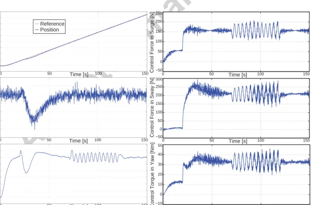
disturbance is still acting on the vehicle. Figures 2 and left column of Figure 3 show the displacements, displacement errors, and velocities in the DOF of interest. As we can see, the actual position and velocities of the vehicle track their reference as per the control design objectives. The controller recover the trajectory tracking even under the action of a constant disturbance, which acts on the vehicle from t = 20s until the end of the simulation. The sinusoidal disturbance produces a bounded error, which vanishes with exponential decay as the disturbance subsides. The control forces and torque are shown in the right column of Figure 3. It can be seen that the control actions are bounded within admissible values.
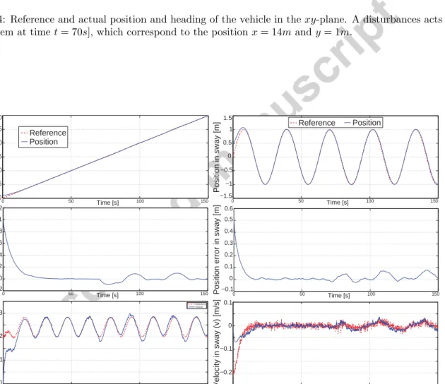
In the second simulation scenario, we consider a sinusoidal trajectory as shown in Fig-ure 4. The vehicle starts at an initial position given by x(0) = 1m, y(0) = 0.5m and
ψ(0) =π/2rad and with no disturbance acting on it. A disturbance is added in the simula-tion att = 70sec. This disturbance is constant in the NED frame but time varying in body-fixed frame. The values of the disturbance forces are set to FN = −10N and FE = −10N,
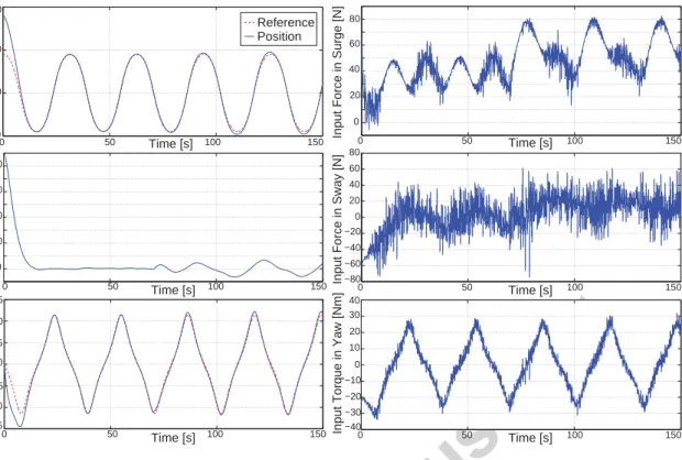
which are the disturbance components in the North and East directions respectively. Figure 4 shows that the vehicle follows the desired trajectory. Figures 5 and left column of Figure 6 show the displacements, displacement errors, and velocities in the DOF of interest. As in the first scenario, the controller shows good performance tracking the references as desired, and ensures ensures exponential convergency of the trajectory error, and bounded error under the action of the disturbance. The control forces and torque are shown in the right column of Figure 6. It can be seen that the control actions are bounded within admissible values.
As shown in simulations, the designed controller demonstrate the stability properties proven and perform satisfactorily for both tracking and disturbance rejection tasks.
6. Conclusions
This paper presents port-Hamiltonian models of marine vehicle dynamics in six DOF in both body-fixed and inertial momentum coordinates. The model in inertial coordinates resembles general port-Hamiltonian model of mechanical systems with a coordinate depen-dent mass matrix. This model opens the possibility of specialising passivity-based control
−4 −3 −2 −1 0 1 2 3 4 Position in surge [m] 0 50 100 150 0 0.1 0.2 0.3 0.4 Time [s] Velocity in surge [m/s] −0.2 −0.1 0 0.1 0.2 0.3
Position error in surge [m]
−4 −3 −2 −1 0 1 2 3 4 Position in sway [m] −0.1 0 0.1 0.2 0.3 0.4 0.5 0.6
Position error in sway [m]
−0.2 −0.1 0 0.1 Velocity in sway [m/s] 150 100 50 0 Time [s] 0 50 Time [s] 100 150 0 50 Time [s] 100 150 0 50 Time [s] 100 150 150 100 50 0 Time [s] Reference
Position ReferencePosition
Figure 2: Reference and measured motion variables for forward motion (left column) and lateral motion (right column). −50 0 50 100 150 200 250
Control Force in Surge [N]
−50 0 50 100 150 200 250 300
Control Force in Sway [N]
−10 0 10 20 30 40 50
Control Torque in Yaw [Nm] 0 50 Time [s] 100 150 200
400 600 800
heading angle [deg]
0 50 100 150 −1 0 1 2 3 4 5 6 7 8
Yaw rate [deg/s]
Time [s] −25 −20 −15 −10 −5 0 5 10
heading error [deg]
0 0 50 Time [s] 100 150 0 50 Time [s] 100 150 Reference Position 150 100 50 0 Time [s] 150 100 50 0 Time [s]
Figure 3: Reference and measured motion variables for heading (left column), and control forces and torque in the DOF of interest.
0 5 10 15 20 25 30 −2 −1 0 1 2 3 4 y [m] x [m] Reference Position Disturbance
Figure 4: Reference and actual position and heading of the vehicle in thexy-plane. A disturbances acts on
the system at timet= 70s], which correspond to the positionx= 14mandy= 1m.
0 5 10 15 20 25 30 −0.2 0 0.2 0.4 0.6 0.8 1 1.2 0 0.1 0.2 0.3 Reference Velocity Position in surge [m] Velocity in surge [m/s] P
osition error in surge [m]
0 50 Time [s] 100 150 0 50 Time [s] 100 150 0 50 Time [s] 100 150 −1.5 −1 −0.5 0 0.5 1 1.5 −0.1 0 0.1 0.2 0.3 0.4 0.5 0.6 −0.2 −0.1 0 0.1 0 50 Time [s] 100 150 Position in sway [m]
Position error in sway [m]
Velocity in sway (v) [m/s] 0 50 Time [s] 100 150 0 50 Time [s] 100 150 Reference Position Reference Position
Figure 5: Reference and measured motion variables for forward motion (left column) and lateral motion (right column).
−50 0 50 100 0 10 20 30 40 −15 −10 −5 0 5 10 15
Heading angle [deg]
Heading error [deg]
Yaw rate [deg/s]
0 50 Time [s] 100 150 0 20 40 60 80 −80 −60 −40 −20 0 20 40 60 80 −40 −30 −20 −10 0 10 20 30 40
Input Force in Surge [N]
Input Force in Sway [N]
Input Torque in Yaw [Nm] 0 50 100 150
Time [s] 0 50 Time [s] 100 150 0 50 Time [s] 100 150 0 50 Time [s] 100 150 0 50 Time [s] 100 150 Reference Position
Figure 6: Reference and measured motion variables for heading (left column), and control forces and torque in the DOF of interest..
strategies developed for mechanical systems for the motion control of marine vehicles, which will be a topic of future research.
The body-fixed coordinate model generalises our previous work in this field. We show how the two models in the two momentum coordinates are related via a momentum trans-formation, and we indicate how these models relate to vector models commonly used in the literature of motion control of marine vehicle dynamics. The body-fixed coordinate model is then used to design a robust IDA-PBC tracking controller. This is a very attractive technique for designing motion controllers for mechanical systems. Having the models in pH form allows to see energy properties of the system, which the designer can choose to preserve. Indeed, in the control design developed in the paper, we choose to maintain the open-loop mass matrix in the kinetic energy component of the error dynamics. We also show how to augment the state and the target Hamiltonian in order to achieve disturbance rejection of fully actuated vehicles. We prove exponential stability in the case of constant disturbances and bounded errors in the case of bounded time-varying disturbances.
Finally, we use simulation example to illustrate the stability properties and the perfor-mance of the controller.
References
[1] R. Ortega, A. van der Schaft, B. Maschke, G. Escobar, Interconnection and damping assignment passivity-based control of port-controlled Hamiltonian systems, Automatica 38 (4) (2002) 585–596.
[2] A. van der Schaft, L2-Gain and Passivity Techniques in Nonlinear Control, Communications and Con-trol Engineering, Springer Verlag, London, 2000.
[3] T. I. Fossen, S. P. Berge, Nonlinear vectorial backstepping design for global exponential tracking of marine vessels in the presence of actuator dynamics, in: IEEE Conf. on Decission and Control, San Diego, 1997, pp. 4237– 4242.
[4] T. I. Fossen, Handbook of Marine Craft Hydrodynamics and Motion Control, Wiley, 2011.
[5] R. Ortega, A. Loria, P. J. Nicklasson, H. Sira-Ramirez, Passivity-Based Control of Euler Lagrange Systems, Springer, 1998.
[6] A. J. Sorensen, O. Egeland, Design of ride control system for surface effect ships using dissipative control, Automatica 91 (32) (1995) 183–199.
[7] C. Woolsey, N. Leonard, Stabilizing underwater vehicle motion using internal rotors, Automatica 38 (12) (2002) 2053–2062.
[8] A. Donaire, T. Perez, Port-Hamiltonian theory of motion control for marine craft, in: 8th IFAC
Conference on Control Applications in Marine Systems, Rostock, Germany, 2010.
[9] A. Donaire, T. Perez, C. Renton, Manoeuvring control of fully-actuated marine vehicles — a
port-Hamiltonian system approach to tracking, in: Australian Control Conference, Melbourne, Australia,
2011.
[10] A. Donaire, T. Perez, Dynamic positioning of marine craft using a port-Hamiltonian framework, Au-tomatica 48 (5) (2012) 851–856.
[11] A. Astolfi, D. Chabra, R. Ortega, Asymptotic stabilisation of some equilibria of an underactuated underwater vehicle, Systems & Control letters 45 (3) (2002) 193–206.
[12] F. Valentinis, A. Donaire, T. Perez, Control of an underactuated-slender-hull unmanned underwater ve-hicle using port-hamiltonian theory, in: IEEE/ASME International Conference on Advanced Intelligent Mechatronics, Wollongong, Australia, 2013.
[13] J. Romero, A. Donaire, R. Ortega, Robust energy shaping control of mechanical systems, System & Control Letters 62 (9) (2013) 770–780.
[14] J. G. Romero, D. Navarro-Alarcon, E. Panteley, Robust globally exponentially stable control for me-chanical systems in free/constrained-motion tasks, in: IEEE Conf. on Decision and Control, Firenze, Italy, 2013.
[15] A. Donaire, J. Romero, T. Perez, Passivity-based trajectory-tracking for marine craft with disturbance rejection, in: IFAC Conference on Manouvring and Control of Marine Craft, Copenhagen, Denmark, 2015.
[16] C. Lanczos, The variational principles of mechanics, 4th Edition, Dover Publications, 1986.
[17] A. van der Schaft, Port-Hamiltonian systems: an introductory survey, in: Proceeding of the Interna-tional Congress of Mathematicians, Vol. 3, 2006, pp. 1339–1365.
[18] R. Ortega, E. Garc´ıa-Canesco, Interconnection and damping assignment passivity-based control: A survey, European Journal of Control 10 (2004) 432–450.
[19] A. van der Schaft, Port-Hamiltonian systems: an introductory survey, in: International Congress of Mathematicians, Madrid, Spain, 2006.
[20] T. I. Fossen, Marine Control Systems: Guidance, Navigation and Control of Ships, Rigs and Underwater Vehicles, Marine Cybernetics, Trondheim, 2002.
[21] D. Greenwood, Advanced Dynamics, Cambridge University Press, 2003.
[22] A. Venkatraman, R. Ortega, I. Sarras, A. van der Schaft, Speed observation and position feedback stabilization of partially linearizable mechanical systems, IEEE Transactions on Automatic Control 55 (5) (2010) 1059–1074.
![Figure 1: Reference and actual vehicle position in the xy-plane. The plots correspond to different time intervals: t ∈ [0s, 63s] (left plot), t ∈ [55s, 110s] (middle plot), and t ∈ [100s, 150s] (right plot).](https://thumb-us.123doks.com/thumbv2/123dok_us/9058276.2803944/14.892.128.786.166.344/figure-reference-actual-vehicle-position-correspond-different-intervals.webp)