Investigation of a Neural Network Approach in Modeling and Diagnostics of an Engine-out NOx Sensor

(1)

Graduate Theses, Dissertations, and Problem Reports

2017

Investigation of a Neural Network Approach in Modeling and

Diagnostics of an Engine-out NOx Sensor

Zackery S. Layhew

Follow this and additional works at: https://researchrepository.wvu.edu/etd

Recommended Citation Recommended Citation

Layhew, Zackery S., "Investigation of a Neural Network Approach in Modeling and Diagnostics of an Engine-out NOx Sensor" (2017). Graduate Theses, Dissertations, and Problem Reports. 6046. https://researchrepository.wvu.edu/etd/6046

This Thesis is protected by copyright and/or related rights. It has been brought to you by the The Research Repository @ WVU with permission from the rights-holder(s). You are free to use this Thesis in any way that is permitted by the copyright and related rights legislation that applies to your use. For other uses you must obtain permission from the rights-holder(s) directly, unless additional rights are indicated by a Creative Commons license in the record and/ or on the work itself. This Thesis has been accepted for inclusion in WVU Graduate Theses, Dissertations, and Problem Reports collection by an authorized administrator of The Research Repository @ WVU. For more information, please contact [email protected].

(2)

Investigation of a Neural Network Approach in Modeling and

Diagnostics of an Engine-out NOx Sensor

Zackery S. Layhew

Thesis submitted

to the Benjamin M. Statler College of Engineering and Mineral Resources

at West Virginia University

in partial fulfillment of the requirements for the degree of Master of Science in

Mechanical Engineering

Arvind Thiruvengadam Padmavathy, PhD, Committee Chairperson Scott Wayne, PhD

Greg Thompson, PhD

Department of Mechanical and Aerospace Engineering

Morgantown, West Virginia 2017

(3)

ABSTRACT

Investigation of a Neural Network Approach in Modeling and

Diagnostics of an Engine-out NOx Sensor

Zackery Layhew

The objective of this study was to develop a method for fault detection of an engine-out oxides of nitrogen (NOx) sensor. The aim of the developed method was not only to isolate a fault with the NOx sensor, but to also diagnose faults in other engine subsystems that may result in higher engine-out NOx production. The developed fault diagnostics are aimed at providing reliable, accurate determinations of sensor output, in-lieu of physical sensors.

The data for the development of numerical models in this study was derived from in-use emissions data of a 2014 Freightliner equipped with a 2013 Cummins ISX15 engine. Data included engine control unit (ECU) data from a variety of vehicle operation in southern California that included interstate, highway, regional, local, and near dock locations.

For this method of fault detection, a virtual sensor was created using an artificial neural network (ANN) with an input configuration using 12 engine parameters, which provided the most accurate results in this study. These parameters included engine speed, engine torque, fuel rate, intake temperature, boost pressure, exhaust temperature, coolant temperature, oil pressure, the first derivative of engine speed, the first derivative of engine torque, the second derivative of engine speed, and the second derivative of engine torque. The neural network could then be used to predict expected NOx values.

(4)

The ANN NOx model was trained on a subset of the data and later validated with another subset of the available ECU data. Two different sets of training data, and seven validation data sets were used for prediction evaluation. The study also included the insertion of fault data and run against the model to test for fault detection with the best performing data set. It was found that the network is able to predict NOx within 1-5% at highway operation, when trained with highway data, enabling the detection of NOx sensor faults as well as faults in engine subsystems that were included in the input parameters for the neural network. Three different types of sensor failures, including a step, ramp, and square function failure, were implemented in the validation data, which caused an increase in error between the actual and predicted NOx production to increase between 15-200%, creating the means of detection.

(5)

iv

ACKNOWLEDGMENTS

I would first like to thank my Committee Chairperson Dr. Arvind Thiruvengadam for providing me with the opportunity to do research in the field of engines and OBD. I would also like to thank my other committee members, Dr. Greg Thompson and Dr. Scott Wayne. A special thank you to Dr. Wayne for everything you have taught me, and the mentorship you have provided throughout my entire undergraduate career, from SAE to Formula to everything else in between.

Next I would like to thank Dr. Melissa Morris, Saroj Pradhan and Pragalath Thiruvengadam for all the help and support in completing my research.

To Pat and Pam, I cannot thank you enough for the support and family-like treatment you have provided in the last two years.

I would like to thank my parents for helping me achieve everything I have so far in my life and shaping me into the person I have become. Without them, I would never have been able to achieve the things I have so far in my life.

Finally, to my wife Emily who has dealt with me spending long days and nights at engineering, and always being as supportive and as helpful as possible. I am thankful to have a true partner.

(6)

v

LIST OF FIGURES

Figure 1-Human Neuron [11] ... 5

Figure 2-Model of a Neuron [9] ... 6

Figure 3-Diagram of Neural Network Layers ... 8

Figure 4-Time Delay Neural Diagram ... 9

Figure 5-Speed Breakdown of Test Data ... 15

Figure 6-Interstate vs. Highway Torque ... 16

Figure 7-Neural Network Diagram ... 20

Figure 8-Performance vs. R Value ... 29

Figure 9-Training Output for Highway 1... 30

Figure 10-Training output for Combined Data ... 31

Figure 11-Scatterplot of Highway 2 Validation Test with NN Trained with Training Data 1 ... 33

Figure 12-Actual vs. Predicted NOx for Highway 3 with 50 Point Smoothing ... 35

Figure 13-Enlarged Actual vs. Predicted for Highway 3 ... 35

Figure 14- Scatterplot of Highway 3 Validation Test with NN Trained with Training Data 1 ... 36

Figure 15- Scatterplot of Regional Validation Test with NN Trained with Training Data 1 ... 39

Figure 16- Scatterplot of Local Validation Test with NN Trained with Training Data 1 ... 41

Figure 17- Scatterplot of Neardock Validation Test with NN Trained with Training Data 1 ... 43

Figure 18- Scatterplot of Interstate 1 Validation Test with NN Trained with Training Data 1 ... 45

Figure 20-Scatterplot of Highway 2 Validation Test with NN Trained with Training Data 2 ... 49

Figure 21- Scatterplot of Highway 3 Validation Test with NN Trained with Training Data 2 ... 52

Figure 22- Scatterplot of Regional Validation Test with NN Trained with Training Data 2 ... 55

Figure 23- Scatterplot of Local Validation Test with NN Trained with Training Data 2 ... 57

(10)

ix Figure 24- Scatterplot of Neardock Validation Test with NN Trained with Training

Data 2 ... 60

Figure 26- Scatterplot of Intersate 2 Validation Test with NN Trained with Training Data 2 ... 64

Figure 27-Step NOx Sensor Failure ... 69

Figure 28-Ramp NOx Sensor Failure ... 69

Figure 29-Square Wave NOx Sensor Failure ... 70

Figure 30-Boost Pressure Sensor Step Failure ... 72

Figure 31-Boost Pressure Sensor Ramp Failure ... 72

(11)

x

LIST OF TABLES

Table 1-1971 ARB Emissions Regulations ... 2

Table 2-Percent Reduction of Pollutants from 1990 to 2015 [7]... 3

Table 3-Description of Tests ... 14

Table 4-Input Configurations ... 19

Table 5-Optimal Neural Network Configuration ... 20

Table 6-Test Matrix with Input Set 1 ... 25

Table 10-Highway 2 Validation Test Errors when Trained with Training Data 1 .... 32

Table 11-R Values for Highway 2 ... 33

Table 12-Highway 2-200 Second Errors... 34

Table 13- Highway 3 Validation Test Errors when Trained with Training Data 1 ... 36

Table 14-R Values for Highway 3 ... 37

Table 15-Highway 3-200 Second Errors... 38

Table 16- Regional Validation Test Errors when Trained with Training Data 1 ... 39

Table 17-Regional R Values ... 39

Table 18-Regional-200 Second Errors ... 40

Table 19- Local Validation Test Errors when Trained with Training Data 1 ... 41

Table 20-Local R Values ... 42

Table 21-Local-200 Second Errors ... 42

Table 22- Neardock Validation Test Errors when Trained with Training Data 1 ... 43

Table 23-Neardock R Values ... 44

Table 24-Neardock Percent Errors ... 44

Table 25- Interstate 1 Validation Test Errors when Trained with Training Data 1 ... 45

Table 26-Interstate 1 Correlation Values ... 45

Table 27-Interstate 1-200 Second Errors ... 46

Table 29-Interstate 2 Correlation Values ... 47

Table 30-Interstate 2-200 Second Errors ... 48

Table 31- Highway 2 Validation Test Errors when Trained with Training Data 2 ... 49

Table 32-Highway 2 Correlation Values ... 50

Table 33-Highway 2 Training Data 2-200 Second Errors ... 51

(12)

xi

Table 35-Highway 3 Training Data 2 Correlation Values ... 53

Table 36-Highway 3 Training Data 2-200 Second Errors ... 54

Table 37- Regional Validation Test Errors when Trained with Training Data 2 ... 55

Table 38-Regional Training Data 2 Correlation Values ... 56

Table 39-Regional Training Data 2-200 Second Errors ... 56

Table 40- Local Validation Test Errors when Trained with Training Data 2 ... 57

Table 41-Local Training Data 2 Correlation Values ... 58

Table 42-Local Training Data 2-200 Second Errors ... 59

Table 43- Neardock Validation Test Errors when Trained with Training Data 2 ... 59

Table 44-Neardock Training Data 2 Correlation Values ... 60

Table 45-Neardock Training Data 2-200 Second Errors ... 61

Table 47-Interstate 1 Training Data 2 Correlation Values ... 62

Table 48-Interstate 1 Training Data 2-200 Second Errors ... 63

Table 50-Interstate 2 Training Data 2 Correlation Values ... 64

Table 51-Interstate 2 Training Data 2-200 Second Errors ... 65

Table 52-Average Percent Errors Table ... 66

Table 53-Average R Values ... 66

Table 54-Error Comparison of Low Power Removed ... 67

Table 55-R Value Comparison of Low Power Removed ... 68

Table 56-NOx Sensor Fault Errors ... 71

Table 57-Boost Pressure Sensor Failure Errors ... 74

(13)

xii

SYMBOLS

AARE Average Absolute Relative Error

ANN Artificial Neural Network

BFG Quasi-Newton

CAFEE Center for Alternative Fuels, Engines and Emissions CARB California Air Resources Board

CGF, CGP, CGB Conjugate Gradient Backpropagation

CO2 Carbon Dioxide

ECU Engine Control Unit

EGR Engine Gas Recirculation

GD Gradient Descent backpropagation

GDm Gradient Descent backpropagation with momentum IMEP Indicated Mean Effective Pressure

ITE Indicated Thermal Efficiency

LM Levenberg-Marquardt

MIL Malfunction Indicator Light

MSE Mean Squared Error

NN Neural Network

NAR Nonlinear Autoregressive

NARX Nonlinear Autoregressive with External

NOP Needle Opening Pressure

NOx Oxides of Nitrogen

NRMSE Normalized Root Mean Square Error

OBD On-Board Diagnostics

RMSE Root Mean Squared Error

SOI Start Of Injection

(14)

1

1 INTRODUCTION

1.1 M

OTIVATION

The motivation for this study was to develop a model that could be used for the advancement of on-board diagnostics (OBD) for heavy-duty diesels. It can be seen in the California Code of Regulations [1] that fault limits decrease from 2010 to 2013, and will continue to decrease as new laws are published. This means that more accurate detection strategies must continue to be developed. The Code of Federal Regulations [2] states that a monitor must be able to make an evaluation within ten seconds and determine if there is a fault. The need for highly accurate, quick evaluation techniques is driving the development of new methods, like explored in this study.

1.2 O

BJECTIVE

The objective of this study is to lay the groundwork for the development of an OBD system using a virtual NOx sensor output and the readings of the engine out NOx sensor. If an accurate model can be developed to predict the NOx production in real time, this value can be compared to the NOx sensor reading to determine if there is either a problem with the NOx sensor or within one of the engine subsystems. A deviation in the prediction and NOx sensor reading may be used for fault detection and identification. The tasks to accomplish the overall objectives are listed below.

• Develop a well performing ANN

(15)

2 • Investigate fault detection of NOx sensor and engine subsystem sensors with the

ANN

1.3 B

ACKGROUND

1.3.1 D

IESEL

E

NGINES AND

E

MISSIONS

The California Air Resources Board (CARB) was created in 1967, after merging the California Motor Vehicle Pollution Control Board and the Bureau of Air Sanitation. There were some studies for the control of smoke and odor began in 1942, with the most significant paper from General Motors in 1956, but it was not until the enactment of Assembly Bill 357 that the Air Resources Board (ARB) was required to develop standards for carbon monoxide (CO), oxides of nitrogen (NOx), and hydrocarbon (HC) emissions. This bill stated that the standards had to be developed by January 1, 1971, and would begin to be enforced January 1, 1973 [3].

Table 1-1971 ARB Emissions Regulations

1971 ARB Emissions Regulations

HC+NOx 16 g/hp-hr

CO 40 g/hp-hr

Ever since the first set of emissions regulations was set in 1971 (Table 1), there has been a continuous push for lower and lower emissions. Heavy duty engines emit four main types of pollutants; CO, HC, NOx, and particulate matter (PM). CO is an odorless, colorless gas, that is poisonous to people and animals [4]. CO forms from incomplete combustion, as a result of less than ideal air and fuel mixture. [5]. CO can cause headache, dizziness, weakness, upset stomach,

(16)

3

vomiting, chest pain, and confusion, and if enough is inhaled it can lead to a person passing out, or death [4]. HC are a result of unburnt fuel in the combustion process. HC are a mix of chemicals that not only contribute to the formation of ozone, but also are toxic to humans and animals and may be a cause of cancer [5]. NOx are produced when combustion temperature is in the 2500-3000 K temperature range [6]. NOx emissions directly contribute to the formation of ozone and have negative health effect on the respiratory system [5]. PM includes particles that are smaller than 2.5 microns and can pass through the nose and upper lungs that can cause irritation in the respiratory system [5].

Emissions regulations are important for the maintenance and improvement of air quality in the United States, and around the world. The Clean Air Act has reduced the levels of six pollutants: PM 2.5, ozone, lead, carbon monoxide, nitrogen dioxide, and sulfur dioxide [6]. Results show five of the six pollutants have reduced by an average of 70% from 1970 to 2015. The exclusion to this is ozone, which has only been reduced by 3%. Table 2 shows the percentage reduction of pollutants in the air from 1990 to 2015 [7].

Table 2-Percent Reduction of Pollutants from 1990 to 2015 [7] Percent Reduction of Pollutants

Lead 85%

Carbon Monoxide 84%

Sulfur Dioxide 67%

Nitrogen Dioxide 60%

Ozone 3%

Fine Particle Concentrations 37% Coarse Particle Concentration 69%

(17)

4

1.3.2 O

N

-

BOARD

D

IAGNOSTICS

On-board diagnostics is computer software that monitors emissions related components in an engine to ensure that everything is operating within the manufacture set range of values. The Clean Air Act Amendments (CAAA) of 1990 was the first OBD requirements [8]. These amendments required the monitoring of the catalyst and oxygen sensor at a minimum [8]. OBD is important to identify failure in any component of emissions control system that can result in higher levels of tailpipe emissions leading to non-compliant operation.

OBD for heavy-duty vehicles began in 2005 and were required for all vehicles over 14,000 pounds (gross vehicle weight rating) in 2013. These requirements include the illumination of a malfunction indicator light (MIL) and the storage of data in the ECU on the faulty component so that it can be downloaded. The primary reason OBD is needed is to regulate components over time. It was reported that the oldest twenty percent of vehicles cause sixty percent of pollution [9]. Other benefits include the early detection of failures and the elimination or unnecessary repairs [9].

CFR 40 86.1806-05.n.3.iii states “(iii) NOxsensors. If equipped, sensor deterioration or malfunction resulting in exhaust emissions exceeding any of the following levels: for 2007 through 2009 model years, 5 times the applicable PM standard, or 4 times the applicable NOx standard and, for 2010 through 2012 model years, 4 times the applicable PM standard, or the applicable NOX standard 0.6 g/mi and, for 2013 and later model years, the applicable PM standard 0.04 g/mi, or the applicable NOX standard 0.3 g/mi.” This rule declares that an OBD system must be able to capture a deteriorating NOx sensor, or any fault that may affect the NOx emissions. The CFR also states in section86.1806-05.n.7 “(7)Performance of OBD functions. Any

(18)

5

sensor or other component deterioration or malfunction which renders that sensor or component incapable of performing its function as part of the OBD system must be detected and identified on engines so equipped.” This rule declares that the functionality of all sensors in the engine must perform within a tolerance to detect any problems in any subsystem of the engine. [2]

1.3.3 A

RTIFICIAL

N

EURAL

N

ETWORK

An artificial neural network (ANN) is a computation system based on the function of the human brain. An ANN consists of parallel computing with interconnections of neurons. The connections between the neurons resemble the connectivity within the human brain as seen in Figure 1 [11].

(19)

6

Figure 2-Model of a Neuron [9]

Figure 2 shows the relation to the neuron in a neural network and how it compares to the biological neuron. The inputs [a1, a2, … an] are multiplied by weights [w1, w2, … wn] in the synapses

and then the summation of the inputs and weight are put through the transfer (or activation) function Ψ in the neuron. The equation for the modified inputs and transfer function can be seen in Equation 1, where o is the output and θ represents a bias value [12].

𝑜(𝑡) = 𝛹[∑ 𝑤_𝑖𝑎_𝑖 + 𝜃

𝑛

𝑖=1

Equation 1-Neuron Transfer Function

There are several transfer functions that can be used within a neural network. These include linear unbounded, unipolar binary, bipolar binary, unipolar linear, bipolar semi-linear, unipolar sigmoid, bipolar sigmoid, multimodal sigmoid, and radial basis. For this study, the hidden layer incorporated a bipolar sigmoid and the output layer incorporated a linear

(20)

7

unbounded transfer function. These two functions are the default function configuration for a time series neural network within Matlab. The transfer functions can be changed to test for added accuracy, but this was not performed in this study. Equation 2 shows the bipolar sigmoid, and Equation 3 shows the linear unbounded, where oj is the output of neuron j, ij is the total

input and α is a constant.

𝑜_𝑗(𝑡) = 𝛹[𝑖_𝑗(𝑡)] = tanh⁡[𝛼𝑖_𝑗]

Equation 2-Bipolar Sigmoid

𝑜𝑗(𝑡) = 𝛹[𝑖𝑗(𝑡)] = 𝛼𝑖𝑗 Equation 3-Linear Unbounded

There are three different types of neurons within a neural network. There are input, output, and hidden neurons. A neural network can have multiple numbers of hidden layers. In this study, only one hidden layer was used. A single hidden layer is most common in neural networks, and is the default in the Matlab toolbox. The hidden layer size was an iterated variable tested for maximum performance that will be outlined in section 2.2.3. The number of neurons in the input and output layers are equal to the number of inputs and outputs used in the data. The number of neurons in the hidden layer is user defined. The number of hidden layer neurons was iterated for accuracy within this study. Figure 3 shows a diagram of the interaction of the three types of layers within the neural network [13].

(21)

8

Figure 3-Diagram of Neural Network Layers

There are several different types of training algorithms used for neural networks. For this study, a backpropagation algorithm was used. A backpropagation algorithm uses two passes to adjust the weights and biases in the neural network. On the forward pass, the weights and biases are not adjusted. The difference between the output and the actual value is propagated backwards to update the weights and biases [14]. The two methods used in this study are Bayesian Regularization (BR) and Levenberg-Marquardt (LM). Both training methods utilize the Levenberg-Marquardt optimization, but Bayesian Regularization creates a network that generalizes well by minimizing a group of squared errors and weights [15]. The Levenberg-Marquardt optimization algorithm can be seen in Equation 4, where J is the Jacobian matrix, k is the time step, I is the identity matrix, µ is the learning rate, and e is the vector of network errors. [16]

(22)

9

Equation 4-Levenberg-Marquardt Optimization Algorithm

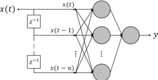
Another aspect of the neural network used in this study consists of the time delay. To better capture the operating state of the engine a time delay was incorporated into the neural network. The term time delay is used in the subject of an ANN to represent which data points are used to make the prediction. A two second time delay would describe the ANN using the data at the current time step and the previous two seconds of data to predict the outcome. In this study, the data was one hertz data so the input delay was equal to time in seconds. This technique is useful in transient situations where a history of the inputs is used for prediction. The time delay goes into the input layer of the neural network which incorporates the previous values to a defined number. Figure 4 shows the incorporation of the previous inputs into the current time step of the neural network [17].

(23)

10

1.4 L

ITERATURE

R

EVIEW

To develop a background of how neural networks have been used in the past, a few different studies were reviewed to evaluate the process of developing a neural network to predict NOx production from an engine.

In a study conducted by Anand et al. [18], they used a neural network to predict NOx emissions and efficiency of a spark ignited biogas engine. Anand et al. created a model using five inputs, which created two outputs. The inputs included, equivalence ratio, compression ratio, spark plug position, engine speed, and carbon dioxide (CO2) fraction. Their neural network

consisted of one hidden layer and varied the number of neurons from two to 12. Anand et al. found that by varying the number of neurons in the hidden layer and measuring the Mean Squared Error (MSE), a hidden layer size of seven neurons provided the best results. While they did not disclose percentages in NOx prediction from their study, a MSE of 7.824e-05 was found from NOx prediction.

A second study by Gadallah et al. [14] used an artificial neural network to predict NOx production and indicated thermal efficiency (ITE) for a direct injection hydrogen engine equipped with water direct injection for NOx control. For the development of the ANN, Gadallah et al. used this study to examine the effects of training algorithms and transfer functions on performance of the neural network. All training algorithms used were backpropagating. The training algorithms included Gradient Descent backpropagation (GD), Gradient Descent backpropagation with momentum (GDm), Conjugate Gradient backpropagation (CGF), (CGP), (CGB), Quasi-Newton (BFG), and Levenberg-Marquardt (LM). Gadallah et al. also used four transfer functions including logistic sigmoid, symmetric logistic, hyperbolic tangent sigmoid, and linear.

(24)

11

To begin their testing, a training algorithm was selected and the number of neurons in the hidden layer was held constant at four. The transfer functions were then iterated for the hidden layer and output layer. The root mean squared error (RMSE) and average absolute relative error (AARE) were recorded for each iteration. The procedure was then repeated varying the number of hidden layer nodes from four to 40. The combination that gives the lowest RMSE and AARE was considered for the best possible solution. This process was conducted for every training algorithm.

Six inputs: equivalence ratio, indicated mean effective pressure (IMEP), hydrogen start of injection (SOI), spark ignition timing, water injection quantity, and water injection timing, were used. The output of the neural network included NOx and indicated thermal efficiency (ITE). The results showed that the Levenberg-Marquardt algorithm, 18 neurons in the hidden layer, hyperbolic tangent sigmoid and linear for the hidden and output layers, respectively, gave the best prediction results.

In another study, Huayi et al. [17] used a multilayer neural network to predict NOx emissions and smoke production in a light-duty turbocharged diesel engine. Huayi et al. considered NOx production at steady state and transient conditions. For steady state prediction engine speed, fueling, main injection timing, injection pressure, intake pressure, intake temperature, and mass air flow were selected. To predict NOx in transient operation engine speed, fueling, intake pressure, intake temperature, mass air flow, and delays of 0.2, 0.4, 0.6, 0.8, and 1 second for fueling, intake pressure, intake temperature, and mass air flow were selected. This resulted in 25 total inputs for transient NOx prediction. For training of the neural network, the Levenberg-Marquardt method was used. The neural network used incorporated two hidden

(25)

12

layers. The neural network was able to predict NOx production with a correlation coefficient of 0.9978.

This study predicted NOx emissions for a two liter, four cylinder, common rail, turbocharged, diesel engine [19]. For the neural network, a total of six inputs were used, including engine speed, engine torque, injection timing, air flow rate, rail pressure, and oil temperature. Zhang et al. used a nonlinear tangent sigmoid function within the hidden layer and a weighted summation within the output layer. The number of neurons in the hidden layer were varied between one and twenty. It was found that with fourteen neurons in the hidden layer, the network showed the best predictions. They concluded that the Normalized Root Mean Square error (NRMSE) was found to be between 5.11 and 8.12 percent difference in predicted versus actual NOx for the four drive cycles tested.

The final study reviewed was based on the development of a neural network for the prediction of NOx from a standard six cylinder, 12 liter heavy-duty EURO-2 engine, at transient operation [20]. The inputs used for the neural network included, engine speed, engine torque, intake pressure, and intake temperature. The intake variables incorporated a time delay different for each variable. Engine speed was used at the current time step and the previous time step. Engine torque included the current time step and the four previous time steps. Intake air pressure was used for the current time step and two previous steps, and no delays were used for the intake air temperature. The number of hidden layers was iterated between zero, one, or two, and the number of neurons was varied between eight and 40. Krijnsen et al. found that the optimal number of hidden layers was one, and the number of neurons within the hidden layer was not clear. With the number of neurons between 20 and 40, the network produced results

(26)

13

between 5-5.5 percent difference between predicted and measured NOx. It was decided that 30 neurons would be used for the study. Upon running the validation data, it was found that there was an average of 6.7 percent error between predicted and actual values for 291 measurements. To investigate the deterioration of a NOx sensor over time, a study conducted by Orban et al. was reviewed [21]. In this study 25 NOx sensors were exposed to exhaust gas for 6000 hours. The sensors underwent calibration checks at the beginning of the test, and after every 2000 hours. The results concluded that depending on the location of the NOx sensor, the degradation of the NOx sensor was between two and 20 percent. This shows the need for a monitor to evaluate the performance of the NOx sensor over the life of the vehicle to ensure accurate NOx readings.

In a study conducted by the US Army Ordnance Center & School and Pacific Northwest Laboratory [22], they explored the use of a neural network to obtain real-time fault diagnostics with more accurate results. In this study derivatives of some input parameter were computed and the neural network functioned in real time within the ECU. This shows the low level of computational intensity of a neural network based on the small number of basic functions used to make the prediction. This study concluded that the use of a neural network would save time and improve diagnostic capabilities.

(27)

14

2 EXPERIMENTAL DATA AND PROCEDURES

2.1 D

ATA

2.1.1 T

EST

D

ATA

All the data used for this study was collected by the Center for Alternative Fuels, Engines and Emissions (CAFEE) at West Virginia University. The data was recorded during in-use vehicle operation in California in 2015. The vehicle used for testing was a 2014 Freightliner implemented with a 2013 ISX15 engine, and an Allison ten speed manual transmission. The testing utilized the same driver for all operation of the truck. The data was broken into eight data sets, dependent on operating states. All cold start and regen operation were excluded for the data used. The data set names and descriptions can be found inTable 3.

Table 3-Description of Tests

Test Name Route Duration

Highway 1 Ontario to Sacramento part 1

5000 sec. Highway 2 Ontario to Sacramento part

2

5100 sec. Highway 3 Ontario to Sacramento part

3

5500 sec Interstate 1 Irvine Route part 1 2850 sec. Interstate 2 Irvine Route part 2 2750 sec.

Regional LA to Ontario 3750 sec.

Local Intermodal Way 4500 sec.

(28)

15

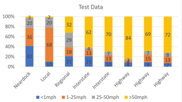
Figure 5-Speed Breakdown of Test Data

As shown in Figure 5 the test data sets contain the percentages of speed breakdown for the data sets. These four ranges were arbitrarily selected to represent idle, city, suburban, and highway driving conditions. These locations consist of vastly different vehicle operations based on percentage of time spent within each speed range. This provided the opportunity to observe how the model would perform during all operating speeds of the vehicle.

42

10

21

10

8

9

7

36

68

18 ₁₃

13

4

15

13

20

29

4

7

3

7 ₈

3

2

32

62 ₇₀

84

69

72 0%

20%

40%

60%

80%

100%

Test Data

<1mph

1-25mph

25-50mph

>50mph

(29)

16

2.1.2 I

NTERSTATE VS

.

H

IGHWAY

D

ATA

C

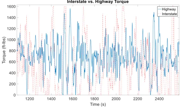
OMPARISON

Figure 6-Interstate vs. Highway Torque

Although the interstate and highway speed breakdown in Figure 5resemble each other, can be seen in Figure 6that torque demand is much different. The torque in the interstate data has larger variations throughout the test than the highway. This means that even though the interstate data resembles highway data from the speed percentage breakdown, the NOx production is different due to the low speed and idle portions mixed throughout the dataset. The low speed and idle portions, mixed throughout the test, create large portions of braking and hard acceleration, which can be seen in Figure 6. With the increased torque demand and engine speed, the NOx production from the engine is much different than that of highway operation.

One objective of this study was to monitor the subsystems of the engine and determine if there was an operating problem. To properly achieve this objective the NOx production for a properly running engine was desired for comparison. All the data collected was from a properly

(30)

17

running engine with no known faults, and excluded operation during cold starts, or when a sensor was not reading properly.

2.1.3 C

OMBINED

T

RAINING

D

ATA

S

ET

For an alternative training method, a combined data set was created. This combined data set consisted of a portion of four different tests. The combined training data set was 3500 seconds of data. The first 500 seconds came from the 500-1000 second portion of the Neardock data set. The next 1000 seconds came from the 1000-2000 second portion of the Regional data set. The following 1000 seconds came from the 1000-2000 second portion of the Interstate 1 data set. The last 1000 seconds came from the 1000-2000 second portion of the Highway 1 data set. This combined data set captured a slice of vehicle operation at many of the locations.

2.2 T

RAINING

2.2.1 M

ODEL

S

ELECTION

There are a variety of types of ANNs. For this study, a prediction of transient data was desired; therefore, a time series type of ANN was required. A Nonlinear Input-Output neural network was chosen. A Nonlinear Autoregressive with External (Exogenous) Input (NARX) or Nonlinear Autoregressive (NAR) type of time series ANN could not be used because of the use of a feedback loop. The feedback loop would enable the model to learn deterioration and drift of the NOx sensor. One objective of this study was to be able to determine NOx sensor failure, which could be in the form of a deterioration drift over time from the true emissions production. With the use of a feedback loop, the neural network would continually learn the output value, meaning that if the sensor developed a drift in either the positive or negative direction, the neural network

(31)

18

would learn this and adjust accordingly. Therefore, the neural network would begin to predict an offset value, eliminating differentiation between the prediction and offset drifted value.

2.2.2 I

NPUTS

The inputs to the network needed to serve two purposes. The first purpose was to give a sufficient amount of detail to make an accurate prediction of NOx production. The second purpose of the chosen inputs was to be a gateway that could be used to monitor engine subsystems. Since proprietary manufacturer data was not available, channels that could represent the amount of Exhaust Gas Recirculation (EGR), Variable Geometry Turbocharger (VGT) position, combustion characteristics, and operating states were desired. This needed to be done with publicly accessible data through the OBD port which was all that was available for this study. For example, intake temperature could be used for detection of changes in EGR position since an increase in EGR flow would cause a change in intake temperature. Eight ECU parameters were chosen to be used in the neural network. The eight parameters chosen were engine speed, engine torque, fuel rate, intake temperature, boost pressure, exhaust temperature, coolant temperature, and oil pressure. The inputs in this study were all engine based, and did not incorporated vehicle parameters. All inputs were normalized between either 0 and 1 or -1 and 1, depending on the nature of the variable.

To further increase the prediction abilities of the neural network, additional forms of the engine speed and engine torque parameters were created. The first and second derivatives along with five-point smoothing of the speed and torque were created. The smoothing was completed using the ‘smooth’ function inside Matlab. The parameters were smoothed due to the high frequency transients throughout the data. The first and second derivatives of the engine speed

(32)

19

and torque parameters were helpful in capturing peaks of NOx production during sudden braking/acceleration occurrences.

Table 4-Input Configurations

Input Configurations

Input Configuration 1 Input Configuration 2 Input Configuration 3 _{Input Configuration 4}

Engine Speed Engine Speed Engine Speed Engine Speed

Torque Torque Torque Torque

Fuel Rate Fuel Rate Fuel Rate Fuel Rate

Intake Temperature Intake Temperature Intake Temperature Intake Temperature Boost Pressure Boost Pressure Boost Pressure Boost Pressure Exhaust Temperature Exhaust Temperature Exhaust Temperature Exhaust Temperature Coolant Temperature Coolant Temperature Coolant Temperature Coolant Temperature

Oil Pressure Oil Pressure Oil Pressure Oil Pressure

First Derivative of Engine Speed First Derivative of Engine Speed First Derivative of Engine Speed First Derivative of Torque Second Derivative of Engine Speed Second Derivative of Engine Speed First Derivative of Torque First Derivative of Torque Second Derivative of Torque Second Derivative of Torque 5-point Smoothing of Engine Speed 5-point Smoothing of Torque

2.2.3 M

ODEL

O

PTIMIZATION

To find the best neural network strategy, a test matrix was constructed. The test matrix iterated different input configurations, delay times, hidden layer size, and computational type. The Pearson Correlation Coefficient (R value) [18] and performance in the form of Mean Squared Error (MSE) were recorded for each of the tests. The R value describes the correlation between the predicted and actual values. An R value of one describes a perfect match between a predicted value and the measured value. R values in between zero and one are broken

(33)

20 into five categories, 0-0.19 is very weak, 0.2-0.39 is weak, 0.4-0.59 is moderate, 0.6-0.79 is strong, and 0.8-1.0 is very strong [23].

Equation 5-Pearson Correlation Coefficient (R Value)

Equation 6-Mean Squared Error

These results can be seen in the Neural Network Development section of the results. The R value and performance were then plotted against each other for evaluation to select the optimal neural network combination. The optimal combination can be seen in Table 5. Figure 7 shows the layout of neural network.

Table 5-Optimal Neural Network Configuration

Inputs Hidden Layer Size Input Delay Training Algorithm

Input Configuration 3 20 2 Bayesian Regularization

(34)

21

2.3 V

ALIDATION

After an ANN combination was selected, it could then be trained. For this study two different sets of training data were used. The first set of training data was Highway 1, and the second set was the combined training data. After the network was trained it could be used to predict NOx on the other data sets. For validation using the first training data set, the Highway 1 data was used for training and then validated against all the other data sets which can be seen in Table 3. This allowed for the complete separation of training and validation data. For validation when the ANN was trained with the combined training data, there was some overlap. The highway portion of the combined training data was excluded since the Highway 1 data was not used for validation, but the other portions had some overlap. Due to the limited amount of data for this study, the Neardock, Regional, and Interstate validation tests, included some overlap with the combined training data. The predicted values could then be compared to the actual data and evaluated. A summed percent error between the predicted and actual values were computed for each of the data sets. A time segment of 200 seconds was arbitrarily selected to sum the actual and predicted NOx values to use for further performance comparison in terms of percent error. Since a neural network prediction will change slightly each time it is trained, the validation tests were performed five times on each data set, retraining the network before each iteration. The validated was run five times to obtain enough values in order to calculate an average representative of the performance with each data set.

2.4 E

XPLORATION OF

P

OOR

P

REDICTION

A

REAS

One hypothesis was that the ANN performed poorly at low power operating states. To explore this hypothesis, all data points in the bottom 20 percent of maximum power were

(35)

22

eliminated from the data sets to be evaluated. The average values of percent error and R for the five iterations of validation testing with and without the low power points were recorded for evaluation.

2.5 OBD

D

EVELOPMENT

Once a neural network had been created, an investigation could be conducted to determine if and when there was a problem with the NOx sensor or one of the ANN input parameters. To begin the fault detection investigation, fault inserted data sets were created to be run against the ANN. Three different types of sensor failure methods were simulated. These three failure methods include a step, ramp, and square wave failure. A ramp failure could simulate a deteriorating NOx sensor that has a reading drifting from the actual value. The step and square wave failures can simulate the failure or loss of communication from the NOx sensor to the vehicle ECU. To investigate the use of the neural network to be able to detect these failures the neural network trained with training data 1, and the Highway 3 data set was used. This combination of neural network and validation data was used since it provided the most accurate prediction. The Highway 3 data set was manipulated to incorporate faults, of the NOx sensor and boost pressure sensor, and compared to the nominal NOx values.

2.5.1 NO

X

S

ENSOR

F

AILURE

For fault detection of the NOx sensor, each of the three failure types had to be simulated in the NOx sensor readings. For the step failure, the value was untouched for the first half of the test and then would step to a value forty percent above nominal value. For the second failure method, a ramp failure was simulated by increasing the value of the reading gradually over the length of the test. The final value would be twenty-five percent above nominal value. The third

(36)

23

failure method would represent the ECU losing connection to the NOx sensor every 400 seconds for 400 seconds. The 400 seconds was arbitrarily chosen just to show the fluctuation of the signal several times over the length of the data set. To simulate this failure method, the NOx values were forced to zero alternating on and off every 400 seconds.

2.5.2 B

OOST

P

RESSURE

S

ENSOR

F

AILURE

The objective of this study was to not only investigate fault detection of the NOx sensor, but to also detect a fault in an engine subsystem. There are sensors in the engine that can change the NOx production if the reading is not correct. Some of these sensors include, the coolant temperature sensor, exhaust temperature, fuel rate, and intake temperature. To investigate the detection of a problem in an engine subsystem the boost pressure channel was selected to be manipulated for this study. The three types of sensor failures were implemented into the boost pressure signal to observe how the neural network prediction would be affected. Like the simulated NOx sensor failure, the boost pressure signal underwent the step, ramp, and square wave function in identical offsets.

(37)

24

3 RESULTS AND DISCUSSION

3.1 N

EURAL

N

ETWORK

D

EVELOPMENT

As discussed in the procedures for optimizing the neural network in Section 2.2.3, a test matrix was constructed to test for the optimal design parameters. The resulting Performance and R value can be seen in Tables 6, 7, 8, and 9.

(38)

25

(39)

26

(40)

27

(41)

28

(42)

29

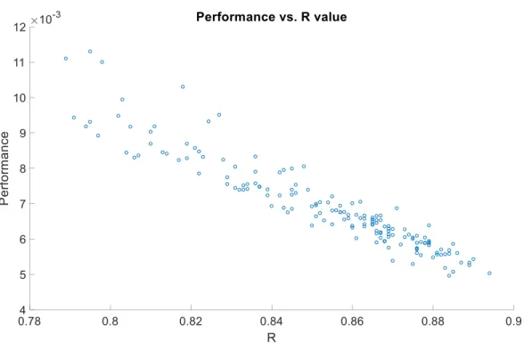
After obtaining the Performance and R value for each of the test combinations, the values could be plotted against each other. Figure 8shows the scatter plot of performance versus R value for the preliminary model tests. A minimal performance value and a maximum R value is desired for the best prediction capabilities. Since the results were linear it was possible to determine which point corresponded to the optimal configuration.

Figure 8-Performance vs. R Value

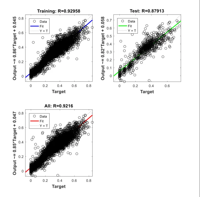
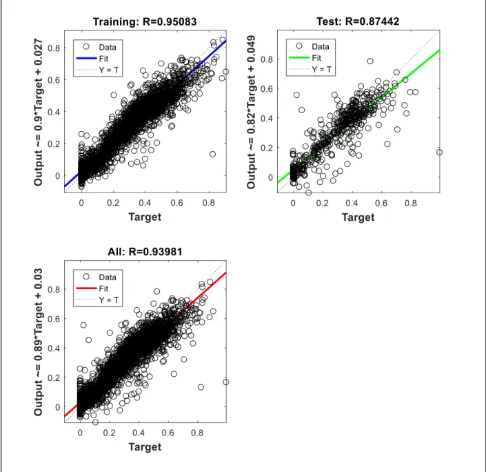
Once a model had been selected, it could be trained. Figure 9 shows the training output when using Highway 1 for the training data, and Figure 10 shows the output of the training data for Training data set 2.

(43)

30

(44)

31

Figure 10-Training output for Combined Data

3.2 T

RAINING

D

ATA

S

ET

1

In this section of the results, the validation tests of the neural network trained with training data set 1 will be shown. The percent error for each of the tests, a correlation plot, the five

(45)

32

correlation values, and the errors in 200 second increments will be shown. The tables include the values for each of the five iterations and the average of these five values. The percent errors calculated are summed errors for the time under evaluation. For the total percent error, the actual and predicted values are summed over the length of the test and then compared. For the error in 200 seconds, the actual and predicted values are summed every 200 seconds and compared. The 200 second increment was arbitrarily chosen for evaluation in a shorter period compared to the length of the test data. The figures depicting the predicted NOx values versus the actual values over time can be seen in Appendix G.

3.2.1 H

IGHWAY

2

The results of the validation testing of Highway 2 can be seen in Table 10. The average error of the five validation tests was 5.37 percent.

Table 10-Highway 2 Validation Test Errors when Trained with Training Data 1

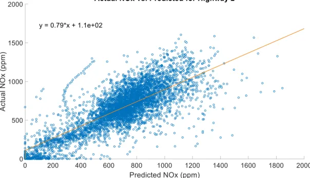
To further describe the performance of the validation of the neural network with the Highway 2 test, the scatterplot of predicted versus actual sensor readings can be seen in Figure 11. This graph shows the correlation of predicted to actual values. The R values for each of the five iterations can be seen in Table 11. The average R value was 0.79 which shows a strong correlation between the predicted and actual values.

(46)

33

Figure 11-Scatterplot of Highway 2 Validation Test with NN Trained with Training Data 1

Table 11-R Values for Highway 2

The last measure of performance was the evaluation of the error in 200 second segments along the test. These values can be seen in Table 12. In the 2001-2201 second range the error is much higher than anywhere else, due to uncharacteristically accelerations within this time period. With a few other exceptions, the error values are below ten percent for all five iterations.

(47)

34

Table 12-Highway 2-200 Second Errors

3.2.2 H

IGHWAY

3

The Highway 3 validation test using training data set 1 had the best results, in terms of percent error, in this entire study. The resulting predicted versus actual sensor readings can be seen in Figure 12. To better observe how the prediction matches the actual values, an enlarged portion of the test is shown in Figure 13.

(48)

35

Figure 12-Actual vs. Predicted NOx for Highway 3 with 50 Point Smoothing

Figure 13-Enlarged Actual vs. Predicted for Highway 3

The percent error values for all five iterations can be seen in Table 13. All five of the tests resulted in less than two percent error over the length of the test.

(49)

36

Table 13- Highway 3 Validation Test Errors when Trained with Training Data 1

Figure 14 shows the correlation of predicted to actual values for Highway 3. The R values for each of the five iterations can be seen in Table 14. The average R value was 0.83, which shows a strong correlation between the predicted and actual values.

(50)

37

Table 14-R Values for Highway 3

Table 15 shows the errors in 200 second increments for the Highway 3 test. In the 2500-2800 and 3400-3600 sections the error is due to uncharacteristic accelerations within these time periods. Excluding these two sections the errors are generally quite low, with almost all sections falling below five percent error.

(51)

38

Table 15-Highway 3-200 Second Errors

3.2.3 R

EGIONAL

Table 16 shows the percent errors for each of the five iterations for the Regional tests. The results for this test were inconsistent with errors ranging between 1.08 and 26.3 percent.

(52)

39

Table 16- Regional Validation Test Errors when Trained with Training Data 1

It can be seen is Figure 15 that there is correlation between the predicted and actual values, but the spread of points is much greater than the Highway tests. Table 17 shows the correlation values for all five iterations.

Figure 15- Scatterplot of Regional Validation Test with NN Trained with Training Data 1 Table 17-Regional R Values

(53)

40

In Table 18, the inconsistency of the prediction is evident. The error percentages range between 69.94 and 0.00 throughout all parts of the test.

Table 18-Regional-200 Second Errors

3.2.4 L

OCAL

The Local validation test resulted in the worst prediction of any test performed, in terms of percent error. The percent error was as high as 70.75 percent for one of the iterations. The error percentages for all the iterations can be seen in Table 19.

(54)

41

Table 19- Local Validation Test Errors when Trained with Training Data 1

Figure 16 shows the correlation between actual and predicted values of the Local test. The correlation values for all the iterations can be seen in Table 20. Although the Local test was the worst performance of the neural network, the average R value was still a 0.6, which means there is still correlation between the actual and predicted values.

(55)

42

Table 20-Local R Values

Table 21 shows how poorly the neural network predicted for the Local test. Errors as high as 155.64 percent can be seen.

(56)

43

3.2.5 N

EARDOCK

The results for the Neardock test show average prediction for this location. The errors for each of the iterations can be seen in Table 22. The errors are higher than the Highway tests but less than the Regional and Interstate tests.

Table 22- Neardock Validation Test Errors when Trained with Training Data 1

Figure 17 shows the correlation of predicted to actual values. The correlation values can be seen in Table 23. The average correlation value is 0.63.

(57)

44

Table 23-Neardock R Values

Table 24 shows the errors in 200 second increments. Since the Neardock data set is much shorter than the rest of the tests, there are less results to compare.

Table 24-Neardock Percent Errors

3.2.6 I

NTERSTATE

1

The Interstate 1 validation test prodcued some interesting results. The average error in the five iterations was 24.29 percent, which can be seen in Table 25. This error value does not describe an entirely accurate prediction, but the average correlation factor between the predicted and actual values is very strong at 0.8, which can be seen in Table 26. Figure 18 shows that while there is a strong correlation between the prediction and actual values, the spread of points ranges much further than the more accurate predictions of the Highway tests.

(58)

45

Table 25- Interstate 1 Validation Test Errors when Trained with Training Data 1

Figure 18- Scatterplot of Interstate 1 Validation Test with NN Trained with Training Data 1

Table 26-Interstate 1 Correlation Values

Table 27 shows that other than a few exceptions, the error is generally between fifteen and thirty percent for all areas of the test.

(59)

46

Table 27-Interstate 1-200 Second Errors

3.2.7 I

NTERSTATE

2

Interstate 2 had similar error results (Table 28) to Interstate 1; however, it can be seen in Table 29 that there is less correlation between the predicted and actual for Interstate 2 (Figure 19).

(60)

47

Table 29-Interstate 2 Correlation Values

Table 30 shows the errors in 200 second increments for Interstate 2. This table shows the variability of a neural network each time it is trained. The errors are fairly consistent except for the third iteration. The third iteration yielded much higher errors than the other four tests. The average error for the third iteration was 42.89% compared to 14.05%, 14.89%, 15.96%, and 13.26%, for iterations one, two, four, and five, respectively.

(61)

48

Table 30-Interstate 2-200 Second Errors

3.3 T

RAINING

D

ATA

S

ET

2

In this section of the results, the validation tests with the neural network trained with the Combined Training Data, training data set 2, will be analyzed. The percent error values, correlation values, and 200 second increment errors will be displayed for each test. The plots for the predicted values versus the actual values can be found in Appendix H.

3.3.1 H

IGHWAY

2

It was found that using training data set 2 caused an increase in error for Highway 2, which can be seen in Table 31. The prediction results are still below eleven percent error for all five iterations, but are higher than when tested with training data set 1.

(62)

49

Figure 20 shows the plot of correlation between predicted and actual values for Highway 2. Table 32 lists the correlation values for all five iterations. The average correlation is 0.76 which is a moderate-strong value.

(63)

50

Table 32-Highway 2 Correlation Values

Table 33 shows the errors in 200 second increments for Highway 2. It can be seen that there are certain areas where the error increases from the results in Section 4.2.1, but also a number of areas still have predictions under five percent.

(64)

51

Table 33-Highway 2 Training Data 2-200 Second Errors

3.3.2 H

IGHWAY

3

The Highway 3 validation test had the biggest effect from switching the training data. By switching the training data Highway 3 changed from the best performing validation test to the worst performing validation test. The percent error increased from 0.926% (Table 13) to 37.24% (Table 34). The correlation coefficient goes from 0.83 (Table 14) to 0.56 (Table 35). This shift in performance can be contributed to the test data compared to the training data. Highway 3 data

(65)

52

is similar to the data in training data 1, but training data 2 includes data from a number of different locations. A plot of the predicted versus actual values can be seen in Figure 21.

(66)

53

Table 35-Highway 3 Training Data 2 Correlation Values

Table 36 shows the 200 second increment errors throughout the Highway 3 test. Iteration 4 is another example of how the results can vary based on training iterations. The results for iteration four are much better than the other iterations, but overall the performance of the prediction was poor compared to the other validation tests.

(67)

54

Table 36-Highway 3 Training Data 2-200 Second Errors

3.3.3 R

EGIONAL

The Regional test using training data 2 begins to show the improvement of the prediction for all the tests except for the Highway tests. The average error of 6.91 percent can be seen in Table 37.

(68)

55

Table 37- Regional Validation Test Errors when Trained with Training Data 2

Figure 22 shows the correlation between predicted and actual values for the Regional test. The correlation values for all five iterations can be seen in Table 38. The average correlation coefficient is 0.82, which means there is a strong correlation between the predicted and actual values.

(69)

56

Table 38-Regional Training Data 2 Correlation Values

Looking at Table 39, extremely high errors can be seen between 2000-2600 seconds. Outside of this range the error appears to be below five percent, with a few exceptions.

(70)

57

3.3.4 L

OCAL

The local validation test produced very inconsistent results. Table 40 shows the errors for each of the five iterations. The error values range from 1.25-16.82.

Table 40- Local Validation Test Errors when Trained with Training Data 2

A plot of the correlation between the actual and predicted value can be seen in Figure 23. The values for the correlation are listed in Table 41.

(71)

58

Table 41-Local Training Data 2 Correlation Values

Table 42 shows how inconsistent the results were for the Local test. In the first 200 seconds two iterations had results of three percent and lower, while another iteration had a 34.48 percent error. In the 2600-2800 section two iterations have error of nineteen percent and higher while two other iterations have an error of 1.95 and below. Section 3400-3600 has a range of errors from 28.19 to 68.18, and the worst section is 2800-3000 where the errors range between 8.21-85.84.

(72)

59

Table 42-Local Training Data 2-200 Second Errors

3.3.5 N

EARDOCK

The Neardock validation test showed decent results. The average of the five iterations was a 6.47 percent error, which can be seen in Table 43.

(73)

60

Figure 24 shows the correlation plot for the predicted to actual values for the Neardock test. The correlation values can be seen in Table 44. The average correlation value was 0.79 which shows a strong correlation.

Figure 24- Scatterplot of Neardock Validation Test with NN Trained with Training Data 2

Table 44-Neardock Training Data 2 Correlation Values

Table 45 shows the error in 200 second increments. The results for the first half of the test (0-600 sec.) resulted in errors less than five percent for every iteration. The last 400 seconds of the test (800-1200 sec.) show a major increase in error. There is an average increase of 19.25% between the first 600 seconds and the last 400 seconds.

(74)

61

Table 45-Neardock Training Data 2-200 Second Errors

3.3.6 I

NTERSTATE

1

Interstate 1 had the best results when the neural network was trained with training data 2, in terms of percent error. The average error was 5.81, shown in Table 46.

(75)

62

Figure 25 shows the correlation between the predicted and actual values. The values for all five iterations can be seen in Table 47. The average correlation value was 0.90 which shows a very strong correlation between the actual and predicted values.

Table 47-Interstate 1 Training Data 2 Correlation Values

Table 48 shows the error every 200 seconds throughout the length of the test. This table shows that other than the first and last 200 seconds of the test the errors are generally under ten percent.

(76)

63

Table 48-Interstate 1 Training Data 2-200 Second Errors

3.3.7 I

NTERSTATE

2

Interstate 2 results resembled the results for Interstate 1. The average error was 7.94, shown in Table 49. The correlation value is slightly lower for Interstate 1, than it was for Interstate 2. The average value for Interstate 2 was 0.82, which is still a strong correlation between the actual and predicted values. The values for the correlation for the five iterations can be seen in Table 50. A plot of the correlation can be seen in Figure 26.

(77)

64

Figure 26- Scatterplot of Intersate 2 Validation Test with NN Trained with Training Data 2

Table 50-Interstate 2 Training Data 2 Correlation Values

Table 51 shows the errors in 200 second increments for the duration of the test. The first 400 seconds show mixed results between the five iterations. The first and fifth iteration show decent prediction during this time; however, the second, third, and fourth iteration have errors between 18-35 percent. The only other area of poor prediction is between 2000-2200 seconds.

(78)

65

Table 51-Interstate 2 Training Data 2-200 Second Errors

3.4 C

OMPARISON OF

T

RAINING

D

ATA

1

TO

2

The average values for percent error and R value for each of the validation tests trained with data set one and two can be used to compare performance. Table 52 gives a good summary to how the neural network predicted values using the different training data sets. When using the highway training data set, resulted in good prediction for the highway validation tests, but a much greater error in all other validation tests. The results for prediction using training data 2 show the opposite results. Using training data 2 caused the prediction of the highway values to decrease, but improved the prediction on all other validation tests.

(79)

66

Table 52-Average Percent Errors Table

Table 53 shows the same results as Table 52. Training data 1 provided good prediction results for the highway tests, but training data 2 improved the results of every other validation test.

Table 53-Average R Values

Table 52 and 53 shows that if highway training data is used, the neural network can predict NOx production within a few percent at highway operation, but suffers greatly for other operating conditions. Changing the training data to a mix of different locations will improve the accuracy of NOx prediction globally, but will not provide the same level of accuracy as highway prediction with highway training, with any validation tests.

(80)

67

3.5 E

LIMINATION OF

L

OW

P

OWER

O

PERATION

To explore the hypothesis that elimination of low power operation the error and R value were evaluated for the validation tests with and without the low power data points. Table 54 shows the comparison of the errors for each data set with and without the low power points. The validation testing with the neural network trained with Training Dataset 1 shows that the error increases in each test except for Highway 3, Local, and Interstate 1. The only test to improve the error by more than one percent was the Local data set. For the validation testing with the neural network trained with Training Dataset 2, only Highway 3 and Local showed a reduction in error. The Local test improved by less than one percent.

Table 54-Error Comparison of Low Power Removed

Table 55 shows the average R values for the validation tests with and without the low power points. With the elimination of the low power points negatively affected the R value for all the data sets.

Investigation of a Neural Network Approach in Modeling and Diagnostics of an Engine-out NOx Sensor

Investigation of a Neural Network Approach in Modeling and

Investigation of a Neural Network Approach in Modeling and

Diagnostics of an Engine-out NOx Sensor

Diagnostics of an Engine-out NOx Sensor

Investigation of a Neural Network Approach in Modeling and

Diagnostics of an Engine-out NOx Sensor

ABSTRACT

Investigation of a Neural Network Approach in Modeling and

Diagnostics of an Engine-out NOx Sensor

ACKNOWLEDGMENTS

Table of Contents

LIST OF FIGURES

LIST OF TABLES

SYMBOLS

1

INTRODUCTION

1.1

M

1.2

O

1.3

B

1.3.1

D

E

E

1.3.2

O

-

D

1.3.3

A

N

N

1.4

L

R

2

EXPERIMENTAL DATA AND PROCEDURES

2.1

D

2.1.1

T

D

42

10

21

21

10

8

9

7

36

68

18

13

13

4

15

13

20

20

29

4

7

3

7

8

3

2

32

62

70

84

69

72

0%

20%

40%

₁₃

₈

₇₀