PERPUSTAKAAN UMP
100
IH IH I0 111 01111111
0000092489
WATER LEVEL FORECASTING USING ARTIFICIAL NEURAL NETWORK IN SUNGAI PAHANG, TEMERLOH
AINUL AFIFAH BINTI ZAKARIA
Report submitted in fulfillment of the requirements For the award of the degree of
B.ENG (HONS) CIVIL ENGINEERING
Faculty of Civil Engineering and Earth Resources UNIVERSITI MALAYSIA PAHANG
ABSTRACT
Flood forecasting models are a necessity, as they help in planning for flood events, and thus help prevent loss of lives and minimize damage. Current studies have shown that artificial neural networks (ANN) which is a parallel computing model have been successfully applied in water level forecasting studies. (ANN) models require historical data of the subject being study. This data is normally separated into a training dataset and a validation dataset. Several performance measures such as Nash-Sutcliffe efficiency, root mean square error and error distribution are used to evaluate forecasting results. BASIC256 software and Microsoft Excel are other way used to implement to ANN modelling technique. The daily water level data can be taken from the Department of Irrigation and Drainage (DID), Malaysia. Water level forecasting is important for environmental protection and flood control since, when flood events occur, reliable water level forecasts enable the early warning systems to mitigate the flood effects. Importantly, the forecasting model developed based on (ANN) successfully achieves high accuracy forecasting result and satisfactory performance result.
ABSTRAK
Kajian yang dijalankan menunjukkan rangkaian neural tiruan (ANN) yang merupakan model perkomputeran selari telah berjaya diaplikasikan dalam kajian ramalan paras air. Model (ANN) memerlukan data paras air yang terdahulu. Data harian paras air telah diambil dari Jabatan Pengairan dan Saliran (JPS) yang dibahagikan kepada dataset latihan dan dataset pengesahan. Beberapa ukuran prestasi seperti NSC, RMSE dan taburan ralat (B) dijalankan untuk menilai ketepatan ramalan. Perisian Basic256 dan Microsoft Excel membantu dalam mendapatkan nilai NSC dan RMSE. Ramalan paras air membolehkan sistem amaran awal seterusnya membantu dalam memelihara alam sekitar dan mengawal banjir. Model ramalan yang dibina berasaskan (ANN) telah berjaya mencapai ketepatan yang tinggi hasil ramalan dan hasil prestasi yang memuaskan.
TABLE OF CONTENTS Page SUPERVISOR'S DECLARATION STUDENT'S DECLARATION ACKNOWLEDGEMENT iv ABSTRACT ABSTRAK vi TABLE OF CONTENTS LIST OF TABLES x LIST OF FIGURES xi
LIST OF ABBREVIATIONS xii
CHAPTER 1 INTRODUCTION
1.1. Introduction 1
1.2. Problem Statement 2
1.3. Objectives of the Study 3
1.4. Scope of Study
1.5. Significance of Study 4
CHAPTER 2 LITERATURE REVIEW
2.1 What is Artificial Neural Network (ANN) 2.2 Neural Network Architecture
VIII
2.2.2 Activation Function 9
2.3 Advantages and disadvantages of (ANN) 9
CHAPTER 3 METHODOLOGY
3.1 Introduction 11
3.2 Artificial Neural Network 11
3.2.1 Sigmoid Function 13
3.3 Datasets 13
3.4 Network Model 14
3.5 Performance Measures 15
CHAPTER 4 RESULTS AND DISCUSSIONS
4.1 Introduction 16
4.2 Forecasting Model 16
4.3 Performance Measures
18
CHAPTER 5 CONCLUSION AND RECOMMENDATION
5.1 Conclusion
23
5.2 Recommendation 24
LIST OF TABLES
Table No. Title Page
4.1 Neural Network Architecture 16
4.2 Data validation and data training with different architecture 17
4.3 Architecture 3-3-1 with different epoch 17
LIST OF FIGURE
Figure No. Title Page
2.1 Feed Forward Network 7
2.2 A 3 layer perceptron 8
3.1 Artificial Neural Network 12
4.1 NSC using Microsoft Excel 18
4.2 RMSE using Basic256 software 20
4.3 Error distribution chart for architecture 3-3-1 at 2000 epoch 21
4.4 Percentage of error distribution for architecture 3-3-1 at 2000 epoch 22
LIST OF ABBREVATIONS
ANFIS Adaptive Neuro Fuzzy Inference System
ANN Artificial Neural Network
ARMA Autogressive Moving Average
ATF Activation Transfer Function
DID Department of Irrigation and Drainage
E Error
MLP-NN Multilayer Perceptron Neural Network
MLP Multilayer Perceptron
NSC Nash-Sutcliffe Efficiency
CHAPTER 1
INTRODUCTION
1.1 Background
Flood is the most significant disaster in Malaysia. Historically, major floods were recorded from 1960 to 2003. The Pahang River Basin which is located in the East Coast of Peninsular Malaysia, usually records heavy rains during November to February due to monsoon season. Sungai Pahang is the longest river in Peninsular Malaysia of about 435 km and drains an area of 29,300 km 2, of which 27,000 km2 lies within Pahang (about 75% of the State) and 2300 km 2 is located in Negeri Sembilan. It is divided into the
Mai
and Tembeling rivers which meet at the confluence near Kuala Tembeling at about 304 km from the river mouth in the central north. Jelai River originates from the Central Mountain Range while Tembeling River has its origin at the Besar Mountain Range.The Pahang river system begins to flow in the south east and south directions from the north passing along such major towns as Kuala Lipis, Jerantut and Temerloh, finally turning eastward at Mengkarak in the central south flowing through Pekan town near the coast before discharging into the South China Sea. Such heavy rains cause flood, which destroys properties, affects economic activities and inundates agriculture lands. Due to the fact that the damages caused by flood are huge, rigorous researches are needed to give an early flood warning system that will save life and properties in the flood affected areas.
Flood forecasting models are a necessity, as they help in planning for flood events,and thus help prevent loss of lives and minimize damage. Current studies have shown that artificial neural networks ANN which is a parallel computing model have been successfully applied in water level forecasting studies. ANN computing is based on the way the human brain processes information. The ANN can define hidden patterns within sample datasets and forecast based on new dataset inputs. Thus, in many areas of study such as forecasting river flow, the ANN does not require defined physical conditions of.the subject, which in this case is the river.
ANN models require historical data of the subject being study. This data is normally separated into a training dataset and a validation dataset. ANN learns the hidden patterns in the historical data through the training dataset. Once the learning process is completed and the knowledge is saved, forecasting can be done using new data input. To verify the success of the data training, forecasting results using the validation dataset are evaluated. Historical records should also be as accurate as possible to ensure reliable forecasting results. Once this is verified, forecasting can be made using the ANN model to produce forecasting result. The accuracy of the results is evaluated using statistical performance model.
1.2 Problem Statement
Flood can occur at any time of the year and are caused by heavy rainfall. Heavy rainfall raises the water level. When the water level is higher than the river bank or the dams, the water comes out from the river, there will be flooding. Besides, flooding can cause death and devastating losses to communities including homes, property and infrastructure. Therefore, flood forecasting is needed to provide better warning for people. The warning process begins when an agency has determined a flood is possible.
1.3 Objectives
1. To predict flood event at Sungai Pahang, Temerloh.
2. To determine whether water level at the station can be used in conjunction with ANN to predict flood event.
3. To determine the neural network parameters that will provide the best prediction for impending floods.
1.4 Scope of Study
This study focuses on water level data that will be recorded at one region, where is in Sungai Pahang,Temerloh. The daily water level data can be taken from the Department of Irrigation and Drainage (DID), Malaysia. Artificial Neural Network (ANN) is one of the most widely used technique in the forecasting field such in this study is to forecast flood event. BASIC 256 software and Microsoft Excel will be used to implement to ANN modelling technique. ANN is used because of its simplicity, easy implementation and demonstrated success in forecasting studies. Several performance measures such as Nash-Sutcliffe efficiency, root mean square error and error distribution are used to evaluate forecasting results.
A flood prediction model can play a key role in providing relevant information of possible impending floods in populated locations. The development of such models can reduce the damage in areas such as by decreasing the economic and environmental impacts of floods. More importantly, a prediction system developed for Pahang River, especially Temerloh area, can effectively lower the risk of harm and loss of life. If artificial neural network (ANN) models can provide sufficiently accurate forecasts, even one day ahead, the subsequent flood emergency measures can be better planned and executed.
Water level forecasting is important for environmental protection and flood control since, when flood events occur, reliable water level forecasts enable the early warning systems to mitigate the flood effects. The ability to forecast water level also helps predict the occurrence of future flooding, enabling better preparation to avoid the loss of lives and minimize property damage. Forecasting studies normally require a series of historical datasets so that future events can be predicted based on past events. It is vital for local agencies such as the water authority to maintain good quality river flow data to facilitate reliable river flow forecasting.
CHAPTER 2
LITERATURE REVIEW
2.1 What is Artificial Neural Network (ANN)
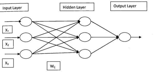
An Artificial Neural Network (ANN) is a parallel-computing mathematical model for solving dynamic nonlinear time series problems. There are many types of ANN, the most common being the multilayer perceptron neural network (MLP-NN) (Zhang et al., 1998) that is used in this study. The architecture of the MLP-NN, shown in Figure 1, contains three types of layer that are ordered in sequence. The first layer is an input layer, the last layer is an output layer and there can be one or more hidden layers in between. Each layer consists of one or more neurons.
The function of the neurons in the input layer is to receive data input and pass this data to the neurons in the second layer. The function of neurons in the hidden and output layers is to receive the input and the weight of input from the neurons in the previous layer and compute the activation transfer function (ATF). There are many types of ATF, and again we use the most common of which is the sigmoid function (Zhang et al., 1998; Maier et al., 2000).
Input= 0 (wx) (1)
The equations for computing the inputs are shown-as above where x is the output from the previous neuron, w is the weight of the output and k is the gradient of the sigmoid function. In most studies, the numbers of input and hidden neurons are determined by trial and error (Coulibaly et al., 2000; Joorabchi et al., 2007; Solaimani and Darvari, 2008; Turan and Yurdusev, 2009).
The number of outputs is normally one, which can be a forecasted week, day or hour, or a forecast at M-hour intervals. The neurons in the network architecture are interconnected between the layers. These interconnections represent the flow of computation in the ANN. The computation process starts from input neurons where data inputs are received, and then propagates to hidden neurons and further to the neurons in the output layer, which produce the model output. The computational process described above is called feed-forward computation.
The process of data training is used to determine the weights. Data training is the process of using sample historical data as the input and output of the network model so that it can simulate the sample data. The training process involves feed-forward and back-propagation computation cycles. Back-propagation computation adjusts the weights of the output and hidden neurons based on the gradient descent method. These weights are normally initialized with random values to speed up the training process. Among the performance measures to evaluate the simulation are mean squared error, root mean squared error and sum of squared error (Zhang et al., 1998).
Once data training is successfully completed, data forecasting can be made with new data input. To evaluate forecasting performance, validation data are used for the input to the network where only feed-forward computation processes the data. Several performance measures are applied to the output of the model and the outputs are Compared with observations from the validation dataset to determine the accuracy and reliability of the network model developed.
2.2 Neural Network Architecture
One class of ANN architecture is the feed-forward network as shown in Figure 2.1. For this class of ANN, data signals always propagate in one direction from the input layer to the output layer and without consideration of any time delays. The neural unit processes the input information. Each of these units is a simplified model of a neuron and transforms its input information into a neuronal output response. This transformation involves the activation of the neuron as computed by the weighted sum of its inputs. This activation is then transformed into a response by using a transfer function.
Ei
utLayer ] I Hidden Layer Output LayerFigure 2.1 Feed Forward Network
The network architecture determines the number of connection weights and also the way information flows through the network. The determination of the best network architecture is one of the difficult tasks in the model building process but one of the most important step to be taken. The ANN models employed in this study are feed-forward networks with hidden layers of neurons. The following neural networks are Commonly used for flood prediction.
8
2.2.1 Multi Layer Perceptrone (MLP)
ML implements feed-forward artificial neural networks or, more particularly, multi-layer perceptronS (MLP), the most commonly used type of neural networks. MLP consists of the input layer, output layer, and one or more hidden layers. Each layer of MLP includes one or more neurons directionally linked with the neurons from the previous and the next layer. The example below represents a 3-layer perceptron with three inputs, two outputs, and the hidden layer including five neurons.
Hidden Input
0
o/)Q
Output(Th><(V
D1
-
Figure 2.2 A 3-layer perceptron
All the neurons in MLP are similar. Each of them has several input links (it takes the output values from several neurons in the previous layer as input) and several output links (it passes the response to several neurons in the next layer). The values retrieved from the previous layer are summed up with certain weights, individual for each neuron, plus the bias term. The sum is transformed using the activation function that may be also different for different neurons.
2.2.2 Activation Function
Activation transfer function (ATF) is the main computing element of ANN and plays an important role in achieving the best forecasting performance. The most common type of activation transfer function is the sigmoid function (Zhang et al. 1998). However, several studies have used different types of ATFs within the ANN to improve the forecasting performance. Shamseldin et al. (2002) used logistic, bipolar, hyperbolic tangent, arc-tan and scaled arc-tan to explore the potential improvement of ANN forecasting. Joorabchi et al. (2007) applied log-sigmoid and hyperbolic tangent sigmoid transfer functions to produce their output. Han et al. (1996) introduced optimization of the variant sigmoid function using a genetic algorithm to optimize the ANN convergence speed and generalization capability.
Many researchers have studied the exterior architecture of the ANN using a trial and error approach. Others have investigated the interior architecture of the ANN, but have been limited to testing different types of ATF in the ANN architecture. The sigmoid function, which is the most commonly used computing function for ATF, has been widely used in the ANN because of its ability to influence the performance of the ANN. The improved performance of the ANN water level forecasting could assist water authorities in managing water resources.
2.3 Advantages and disadvantages of ANN
The ANN learns how to relate the inputs to the outputs without being given any explicit equations when compared with other method, such as K-Nearest Neighbour and ARJ4A method. The only real requirements for the ANN model are for sufficient data for flood modelling events, and the specification of appropriate neural network parameters values to be used. ANNs have relatively low computational demands and can easily be integrated with other techniques. They perform tasks that a linear programme cannot, and when an element of the neural network fails, it can Continue without any problem due to their highly parallel nature [Openshaw and Openshaw, 1997].
Disadvantage of ANNs is that the optimal form or value of most network design parameters can differ for each application and cannot be theoretically defined in general. However, these values are commonly approximated using trial and error approaches [Kumar et al., 2004]. The other disadvantage of neural networks is that they require training to operate,and this may require much processing time for large neural networks [NeuroAI2007, 2007]. Hence the neural network as non-linear model is a promising approach compared to linear models for flood forecasting. As indicated by the results found during this research, their performance results are comparable with other prediction modelling techniques.
CHAPTER 3
RESEARCH METHODOLOGY
3.1 Introduction
In this study, an artificial neural network will be analyzed to forecast water level in Pahang River, Temerloh station. Several performance measures such as Nash-Sutcliffe efficiency, root mean square error and error distribution are used to evaluate forecasting results. BASIC 256 software and Microsoft Excel are other way used to run ANN. Data that will be used in our study is daily water level data. The daily water level data can be taken from the Department of Irrigation and Drainage (DID), Malaysia. Data from year 2003 to 2009 are taken for forecasting result.
3.2 Artificial Neural Network
Artificial Neural Network (ANN) is a parallel computing mathematical solutions for solving linear and nonlinear problems. The modeling algorithm of ANN is based on imitation of how human brain performed. ANN is built based On interconnection between input layer, hidden layer and output layer. Data are assigned at the input layer, and the number of data input is depends on the problem of being solved. Before the ANN model can process the input data, the data are usually normalized or scaled to values between 1 to —1 or 0 to 1. The processing of data starts from the input layer and propagates to hidden layer.
12
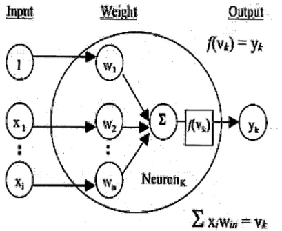
In the hidden layer, there are neurons that processed the data input and weight of the input to the neuron and convert the inputs into an output through activation function. The output of the activation function will become an input to next layer either another hidden layer or output layer. .Sigmoid, linear, step and sign functions are among activation functions that are commonly use in ANN computing. A bias value of one is included as an input to the neurons to make adjustment on the result of activation function. An artificial neuron is shown in Fig. 3.1. At final stage of the computation, the computed output from the output layer is compared to an output of an actual data, and adjustments are made to neuron weights in a backward form. This process is called back propagation learning processes.
Input Weight Oiipit
=
NY
'I I
x1
j
\
p(wJ Neu "on1/
XWfrj:Vk
Figure 3.1 An artificial neural network (Sulaiman M et al. 2011)
Each adjustment to neuron weights and computation from an input to an output layer is called an epoch or iteration. The number of epoch depends on the number chosen by user. Attempt is made so that the computed output is to have a similar result of the actual output data. The whole process of computation and learning is called a training process. Once training is completed, the knowledge acquired is stored in the neuron weights.
Based on this knowledge, forecasted data are assigned as input and computation process propagated from the input to the output layer through the hidden layer. The computed output is called forecasting result. There are many models of ANN and the models are defined based on the network structure of the neurons, connection strengths and processing performed at computing elements or neurons. The most common of ANN model is Multi Layer Perceptron Neural Network (MLP-NN).
3.2.1 Sigmoid Function
The activation transfer function (ATF) forces incoming values to range between o to land ito-i depending on the type of function used. The most commonly used ATF in the ANN is the sigmoid function The sigmoid function is a differentiable function in which the gradient method can be applied to the ANN to adjust the ANN weights so that the model output and observed data reach a target performance value during data training.
y =11(1 + e-kx (3)
The sigmoid function is defined as above, where y is the sigmoid value, k is the sigmoid steepness coefficient and x is the data or incoming values. As in the case of the neural network, the incoming values are the summation of the input and weight values. Additional input with a value of i and its weights are added as a threshold value so that the computed sigmoid function will result in an activation value between 0 and 1.
3.3 Datasets
Hourly historical water level data from the period 2003-2009 were collected from the Department of Irrigation and Drainage (DID). The data was divided into training and validation datasets. The dataset is organized into sets of inputs and output where the number of data inputs depends on the network requirements. In this study, the number of inputs ranges from three to seven water level observations prior to the forecasted period.
The reason a minimum of three data inputs are used to determine the best number of inputs for forecasting is that pre-analysis using less than three data points resulted in a poorer forecasting performance than using three or more data inputs. This could be because there are not enough patterns in the data when using fewer inputs. On the other hand, pre-analysis using more than seven inputs did not improve forecasting performance, possibly due to too many input patterns causing the loss of a distinct pattern within the training dataset. The results presented in this study use from three to seven data inputs, which is reasonable for developing a water level forecasting model.
3.4 Network model
This study uses network models with the following features. One hidden layer is used, since this is adequate for approximating non-linear equations, based on the universal approximation theorem (Homik et al., 1989; Maier and Dandy, 2000). The number of input neurons is the same as the number of the data inputs, and the number of neurons in the hidden layer is the same as the number of neurons in the input layer. Preanalysis using more hidden neurons than input neurons did not produce any significant improvement in forecasting performance, but it was apparent that more hidden neurons made the data training process slower.
The activation transfer function used in the hidden and output neurons is the sigmoid function. We stop the data training process in this study when there is no improvement to the data training performance. Many ANN studies have reported that this approach could cause over-fitting, that is, the performance of the data training increases while the validation performance deteriorates. In this study, a small number of hidden neurons are used to avoid over-fitting. The final data forecasting performance is Compared to the data training performance to verify that over-fitting does not occur. Data training performance is evaluated using Nash-Sutcliffe efficiency.
3•5 Performance Measures
Performance of the forecasting models were evaluated using Nash-Sutcliffe efficiency coefficient (NSC) and root mean square error (RMSE).
(QO-Qm)"2
NSC=1— >(QO-Qmean)"2 (4)
RMSE = p.xQO-Qm)"2 (5)
The equations for these are shown above, where Q ° is observed value, Qm is modelled value, Qmean is mean of the observe value and N is the number of records evaluated. Each of the performance measure will be analysed and it will determine either the data is suitable to be. used or not. Additional performance measures which include in this study is error distribution. Error distribution is calculated by finding the difference between modelled and observed water levels data.
Error = (Q° - Qm) (6)
The equation is as above, where Qm is modelled value and Qo is the observed value. The value obtain describes the precision of the forecasting results in physical values, which will help . water authorities to more understand and sense the accuracy of the forecasting model developed.
CHAPTER 4
ANALYSIS AND DISCUSSION
4.1 Introduction
The result of water level forecasting using (ANN) that have been conducted are presented in this chapter. The goals of this project were to determine whether water level at the station can be used in conjuction with ANN to predict flood event in Sungai Pahang, Temerloh and neural network parameters that will provide the best prediction for impending floods:
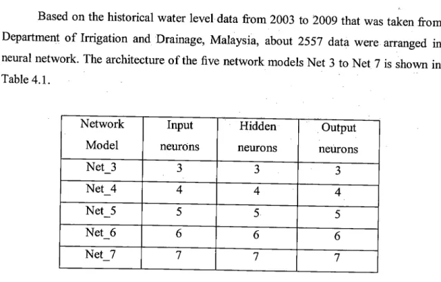
4.2 Forecasting Model
Based on the historical water level data from 2003 to 2009 that was taken from Department of Irrigation and Drainage, Malaysia, about 2557 data were arranged in neural network. The architecture of the five network models Net 3 to Net 7 is shown in Table 4.1. Network Model Input neurons Hidden neurons Output neurons Net-3 3 3 3 Net-4 4 4 4 Net-5 5 5 5 Net-6 6 6 6 Net _7 7 7 7