550 Technical Gazette 27, 2(2020), 550-557
Entropy based Software Reliability Growth Modelling for Open Source Software Evolution
Abhishek TANDON, Meera SHARMA, Madhu KUMARI, V. B. SINGH
Abstract: During Open Source Software (OSS) development, users submit "new features (NFs)", "feature improvements (IMPs)" and bugs to fix. A proportion of these issues get fixed before the next software release. During the introduction of NFs and IMPs, the source code files change. A proportion of these source code changes may result in generation of bugs. We have developed calendar time and entropy-dependent mathematical models to represent the growth of OSS based on the rate at which NFs are added, IMPs are added, and bugs introduction rate.The empirical validation has been conducted on five products, namely "Avro, Pig, Hive, jUDDI and Whirr" of the Apache open source project. We compared the proposed models with eminent reliability growth models, Goel and Okumoto (1979) and Yamada et al. (1983) and found that the proposed models exhibit better goodness of fit.
Keywords: entropy; feature improvement; new feature; open source software 1 INTRODUCTION
OSS evolution is based on the bug triaging process where different reports about the issues are filed. The various attributes related to the issues are also filed during the reporting. The reported issues are assigned to different developers for fixing. The issues which are reported by the users are mainly NFs, IMPs and bugs [28].
In line with the OSS architecture model proposed in [1], we expanded it by incorporating requests, namely feature improvements shown as green colour boxes in Fig. 1. Fig. 1 shows that to fix different issues, developers modify the source code which may result in bugs. In order to fix the issues a lot of changes must be made in the source code. These modifications to the source code were quantified using measurement dependent upon entropy called the "complexity of code changes" [2, 3]. Code changes are quantified based on Shannon entropy [6]. Cobb-Douglas based two dimensional and three dimensional models have been proposed to predict the entropy of software systems by considering bugs, NFs and IMPs [13].
Figure 1 A classification of open source users and developers [1]
In this paper, we proposed calendar time and entropy based models for a software product to estimate the number of issues fixed and to predict the leftover issues which need to be fixed over a long run. The models consider different rates at which different issues are fixed and the rate at which bugs are generated during fixing of these issues.
We have taken into consideration two existing SRGMs [11, 12] to compare with our proposed models. The existing and proposed models have been validated using data collected from the various products of Apache open source project. Results show that the proposed models exhibit better goodness of fit.
In this paper, we have extended the work proposed in [28]. The authors presented a model to represent the OSS growth using the IMPs rate due to fixing of NFs and IMPs. The proposed models have been validated on five products, namely "Avro, Pig, Hive, jUDDI and Whirr" of Apache project.
The remaining part of the paper has been divided into 5 sections. A review of the available literature related to the proposed work in the paper has been presented in section 2. In section 3, the data collection and the mathematical formulation to embody the OSS development have been proposed. Experimental setup has been presented in section 4. The numerical illustrations to validate the proposed models presented in section 5. The paper has been concluded in sections 6.
2 RELATED WORK
Many current OSS quality models come from the standard scheme ISO 9126 [29, 30]. Many different models of open source efficiency and maturity, and their comparative analysis is available in [31].
In a study [32] it was reported that a majority of OSS quality assurance models primarily concentrate on data-dominant software evaluations. A study proposed a framework of process to address the challenges for the evaluation and selection of OSS [33]. The evolution of OSS is characterized by the number of issues that are reported or requests made for their enhancements. The major requests made by users are for the NFs and IMPs in addition to the bugs reports. Therefore, when to release open source software depends not only on the bugs fixed, but also on NFs and IMPs implementation. In OSS
development paradigm software are released frequently without waiting to fix all the requested features [10]. A study has been proposed by incorporating uncertainties in the SRGM [14]. A model based on Dempster-Shafter theory and improved differential evolution has been proposed for allocation of reliability growth and predefined budget in multimedia systems [15]. An optimal release time problem by applying risk-reduction approach with the delay incurred cost has been proposed in [16]. Multi-criteria based dynamic selection model has been used to improve a software reliability prediction model [17]. The modelling of the software correction process consists of bug detection and correction process. After a fault is found the bug correction process will be delayed for some time. By considering these factors, a model has been proposed and validated in [18].
A testing effort and multivariate function based fault prediction rate has been proposed for SRGM [19]. Recently, entropy based SRGMs were proposed to measure the software reliability growth and these models were further used to predict software release time [23, 34]. In another studies [4, 25] remaining software faults from previous release and current faults based multirelease SRGM has been proposed.
Here, a quantified approach for multi version software system has been proposed by considering the NFs and IMPs implementations and bugs generated from these implementations. The proposed model based on Non Homogenous Poisson Process(NHPP), which has been widely used in SRGM [7, 8, 9, 20, 27]. Our model is unique and has the novelty in the sense that it incorporates the rates at which NFs and IMPs are introduced and the bugs generated from the introduction of NFs and IMPs. Our proposed model is an improved model and quite different from the models proposed in [7, 8, 9, 20, 21, 22, 27].
3 DESCRIPTION OF DATASETS AND MODEL CONSTRUCTION
In this section, different datasets used to validate the proposed models followed by the proposed models have been described.
3.1 Description of Datasets
Apache open source products data has been used to validate the proposed models [5].
Tab. 1 shows the data collection time period of different Apache products considered for study.
Table 1 Data collection time period of different Apache products [23] and [28]
Apache products Time period
Avro July 2009 to July 2014
Hive April 2009 to April 2014
Pig April 2009 to October 2013
jUDDI Feb 2009 to Feb 2014
Whirr Sept 2010 to April 2013
Tab. 2 shows the versions for which we have taken the cumulative data and renamed as different release numbers [23].
Once the different issues are reported by the users, these issues are fixed by modifying the code in different files of the software products. Due to these modifications
in the code , the complexity of code changes increases and hence an uncertainty arises. This measure of uncertainty is called entropy.
Table 2 Different versions taken as releases for different Apache products
Release
Number Avro Pig Apache products Versions Hive jUDDI Whirr
Release 1 1.3.2 0.5.0 0.4.1 3.0.1 0.4.0
Release 2 1.5.0 0.8.0 0.6.0 3.1.0 0.7.0
Release 3 1.6.3 0.9.2 0.8.1 3.1.3 0.7.1
Release 4 1.7.4 0.10.0 0.10.0 3.1.5 0.8.1
Release 5 1.7.7 0.12.0 0.13.0 - -
Based on information theory [6], the "complexity of code changes/Entropy" was firstly proposed by Hassan [2]. Shannon entropy [6] is defined as:
2 1 1 ( ) log 0 and 1 n n i i i n i i i H X P P P P = = = − ≥ =
∑
∑
Normalizing Shannon's entropy results in Normalized Static Entropy, H defined as
( )
( )
2 2 2 1 1 1 1 ( ) 1 1 ( log ) log log ( log ) where 0, 1, 2, , and 1 n n n i i i n i n i i n i i i H X H XMax Entropy for Distribution
H X p p n n p p p i ... n p . = = = = ⋅ = ⋅ = ⋅ − ∗ = − ∗ ≥ ∀ ∈ =
∑
∑
∑
t i hnumber of timesi file has beenchanged in a time period the total number of changes in all the fil
p
es during that time period =
3.2 Developing Models For Multi Release Software Product
In OSS, once the issues are reported, the triaging takes place and different issues are assigned to developers. Once the issues are fixed, the source code modifies and in result of this new releases take place. But, there are some issues which are still left in the current release, which get fixed in the next release. A mathematical model is necessary here, which will predict the issues that can be fixed over a long period of time. It is important to note that all issues of the current release could not be fixed due to time constraint and can be remained unresolved and added to the next release.
The proposed models have been compared with Goel-Okumoto model [11] given in (1) and Yamada delayed S-shaped model [12] given in (2).
(
)
( ) 1 exp( ) Y t =i − −bt (1)(
)
( ) 1 (1 )exp( ) 0 Y t =i − +bt −bt i, b > (2)Y(t) cumulative number of fixed errors at any time t; i -potential errors; b - rate of error fixing per remaining error.
552 Technical Gazette 27, 2(2020), 550-557
NHPP based time-dependent SRGMs have been proven to be successful models for quantitative quality evaluation of the software products [7, 26].
Let N(t) denote the total number of issues detected at time t, and Y(t) denote its expectation. Then Y(t) = E[N(t)], and the failure rate λ(t) are related as follows:
0 ( ) = ( )dt Y t
∫
λ t t (3) and d ( ) ( ) d Y t t t =λ (4) Here, i denotes the different issues, i.e. the sum of bugs, NFs and IMPs reported in the issue tracking system. These issues are fixed by active users. Let the rate at which new features are introduced be p and the rate at which feature improvements are incorporated for these new features introductions, be q. It has been assumed that fixing of these issues may result in bugs. Let r be the rate of bugs generated from the introduction of new features fixed out of total issues and s be the rate of bugs generated from feature improvements. This results in the following equation:(
)
(
)
(
)
(
)
d ( ) ( ) ( ) ( ) + d ( ) ( ) + ( ) + ( ) Y t p i Y t qY t i Y t t i prY t i Y t qsY t i Y t i i = + ⋅ ⋅ − ⋅ − − − (5)The number of issues fixed at any time t is denoted by Y(t). In the above Eq. (5), the number i − Y(t) represents the left over issues at time t. p(i − Y(t)) is the number of new features introduced with rate p in the software.
( ) ( ( ))
qY t i Y t
i ⋅ − is the number of feature improvements
incorporated with rate q for the new features added with rate p. prY t i Y t( ) ( ( ))
i ⋅ − is the number of bugs generated
with rate r from the addition of new features added with rate p. qsY t i Y t( ) ( ( ))
i ⋅ − is the number of bugs generated with
rate s from the feature improvements incorporated with rate q. Solving (5) at t = 0, Y(t) = 0 results in the following equation:
(
)
(
)
(
)
(
)
(
)
1 exp (1 ) (1 ) ( ) 1 1 exp (1 ) (1 ) p r q s t Y t i q s rp p r q s t p q − − + + + = + + + − + + + (6)For nth release, Eq. (6) can be written as
( )
(
)
(
)
( )(
)
1 exp (1 ) (1 ) ( ) 1 1 exp (1 ) (1 ) n n n n n n n n n n n n n n n n n n n p r q s t Y t i q s r p p r q s t p q − − + + + = + + + − + + + (7)where Yn(tn) is the issues fixed at any time tn in nth release.
in is the potential issue to be fixed over a long run in the nth
release. pn and qn are the rates at which new features and
improvements in features are introduced in the nthrelease
of the software. rn and sn are the rates of bugs generations
from the incorporation of these new features and improvements in features.
The model given in (6) can also be written in the following form: ( ) ( ) Y t =iG t and
(
)
(
)
(
)
(
)
(
)
1 exp (1 ) (1 ) ( ) 1 1 exp (1 ) (1 ) p r q s t G t q s rp p r q s t p q − − + + + = + + + − + + + (8)where, G(t) follows a distribution function, at t = 0, G(0) = = 0 and at t = ∞, G(∞) = 1.
For nth release, Eq. (8) can be written as:
( )
(
)
(
)
( )(
)
1 exp (1 ) (1 ) ( ) 1 1 exp (1 ) (1 ) n n n n n n n n n n n n n n n n n n p r q s t G t q s r p p r q s t p q − − + + + = + + + − + + + (9) The issues that can be fixed over the long run can be predicted by using the model given in Eq. (6).In the following section, we have assimilated the code changes in order to fix different issues. Eentropy based model for issues prediction has been proposed by considering the code changes in the software.
In the line of proposed model given in (6), we have developed the following entropy i.e. H(t), based model for issues prediction. Y(H(t)) is the mean value function. This results in (10): ( )
(
(
( ))
)
( )(
)
1 exp (1 ) (1 ) ( ) ( ) 1 1 exp (1 ) (1 ) ( ) p r q s H t Y H t i q s rp p r q s H t p q − − + + + = + + + − + + + (10)A software is evolved with its multi-versions. For each version the issues are reported by open source community to meet their own requirements. It is not possible to fix all the reported issues in the current version of the software, therefore the remaining issues are carried over for the next release. The equation given in (6), has been used to evaluate the mean value of the issues.
In order to express mathematically the different releases of the software where a proportion of issues of a long run fixed in the current release and remaining issues passed on to the next release, we formulated the Eq. (11), Eq. (12), Eq. (13), and Eq. (14). The following models presented in Eq. (11), Eq. (12), and Eq. (13) are for Release 1, Release 2, Release 3 and Eq. (14) represents for the nth
release of the software product [4, 23, 24].
1 1
( ) ( ), 0
The number of issues which will be addressed over the future for the first release is i1 at time t1. The quantity i1(1
– G1(t1)) is the leftover issues of Release 1 and it will be
added to the Release 2 to be fixed at the rate G2(t – t1). The
following expression presents the issues for the Release 2.
(
)
(
)
2( ) 2 1 1 1 1( ) 2( 1), 1 2
Y t = i i+ −G t G t t− t ≤ <t t (12) Here, the number of issues over long run to be fixed in Release 2 is i2.
The cumulative number of issues fixed for Release 3 by considering the leftover issues of just previous release is given by:
(
)
(
)
3( ) 3 2 1 2 2( ) 3( 2), 2 3
Y t = i i+ −G t G t t− t ≤ <t t (13) Here, the number of issues over long run to be fixed in Release 3 is i3.
Table 3 Issues based release planning
Issues (Bug, NFs and IMPs) based Release Planning Case 1 Issues Prediction based on Eq. (1)
Case 2 Issues Prediction based on Eq. (2)
Case 3 Issues Prediction based on proposed model given in Eq. (6) Case 4 Issues Prediction based on entropy given in Eq. (10)
Based on the approaches applied for the issues fixing modelling for Release 1, Release 2 and Release 3, the following mathematical equation for nth release can be
written.
(
)
(
1 1 1)
1 1 ( ) 1 ( ) ( ), n n n n n n n n n Y t = i +i− −G− t − G t t− − t− ≤ <t t (14)Similarly, entropy based mathematical expressions for different releases can be derived. The following equation shows the entropy based cumulative modelling for nth
release.
( ( ))
(
1(
1 1( ( 1)))
)
( ( ) ( 1) , ) 1n n n n n n n n n
Y H t = i i+ − −G− H t− G H t H t− − t− ≤ <t t (15)
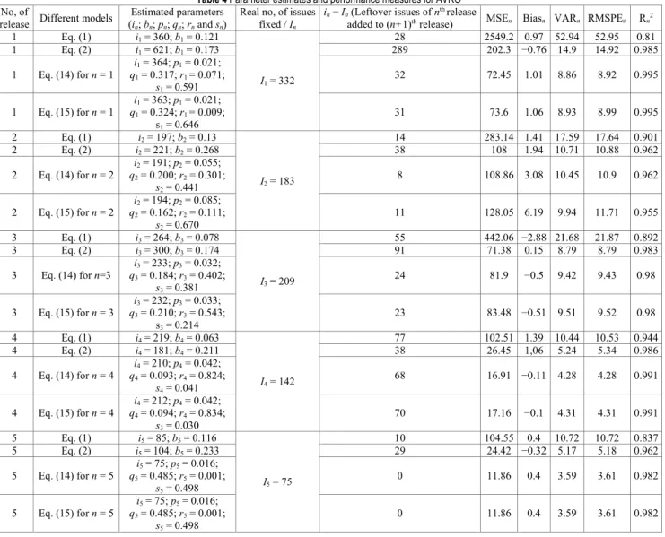
Table 4 Parameter estimates and performance measures for AVRO
No, of
release Different models (Estimated parameters in; bn; pn; qn; rn and sn)
Real no, of issues fixed / In
in−In (Leftover issues of nthrelease
added to (n+1)th release) MSEn Biasn VARn RMSPEn Rn2
1 Eq. (1) i1 = 360; b1 = 0.121 I1 = 332 28 2549.2 0.97 52.94 52.95 0.81 1 Eq. (2) i1 = 621; b1 = 0.173 289 202.3 −0.76 14.9 14.92 0.985 1 Eq. (14) for n = 1 qi11 = 0.317; = 364; p1r = 0.021; 1 = 0.071; s1 = 0.591 32 72.45 1.01 8.86 8.92 0.995 1 Eq. (15) for n = 1 qi11 = 0.324; = 363; p1r = 0.021; 1 = 0.009; s1 = 0.646 31 73.6 1.06 8.93 8.99 0.995 2 Eq. (1) i2 = 197; b2 = 0.13 I2 = 183 14 283.14 1.41 17.59 17.64 0.901 2 Eq. (2) i2 = 221; b2 = 0.268 38 108 1.94 10.71 10.88 0.962 2 Eq. (14) for n = 2 qi22 = 0.200; = 191; p2r = 0.055; 2 = 0.301; s2 = 0.441 8 108.86 3.08 10.45 10.9 0.962 2 Eq. (15) for n = 2 qi22 = 0.162; = 194; p2r = 0.085; 2 = 0.111; s2 = 0.670 11 128.05 6.19 9.94 11.71 0.955 3 Eq. (1) i3 = 264; b3 = 0.078 I3 = 209 55 442.06 −2.88 21.68 21.87 0.892 3 Eq. (2) i3 = 300; b3 = 0.174 91 71.38 0.15 8.79 8.79 0.983 3 Eq. (14) for n=3 qi33 = 0.184; = 233; p3r = 0.032; 3 = 0.402; s3 = 0.381 24 81.9 −0.5 9.42 9.43 0.98 3 Eq. (15) for n = 3 qi33 = 0.210; = 232; p3r = 0.033; 3 = 0.543; s3 = 0.214 23 83.48 −0.51 9.51 9.52 0.98 4 Eq. (1) i4 = 219; b4 = 0.063 I4 = 142 77 102.51 1.39 10.44 10.53 0.944 4 Eq. (2) i4 = 181; b4 = 0.211 38 26.45 1,06 5.24 5.34 0.986 4 Eq. (14) for n = 4 qi44 = 0.093; = 210; p4r = 0.042; 4 = 0.824; s4 = 0.041 68 16.91 −0.11 4.28 4.28 0.991 4 Eq. (15) for n = 4 qi44 = 0.094; = 212; p4r = 0.042; 4 = 0.834; s3 = 0.030 70 17.16 −0.1 4.31 4.31 0.991 5 Eq. (1) i5 = 85; b5 = 0.116 I5 = 75 10 104.55 0.4 10.72 10.72 0.837 5 Eq. (2) i5 = 104; b5 = 0.233 29 24.42 −0.32 5.17 5.18 0.962 5 Eq. (14) for n = 5 q5i = 0.485; 5 = 75; p5r = 0.016; 5 = 0.001; s5 = 0.498 0 11.86 0.4 3.59 3.61 0.982 5 Eq. (15) for n = 5 q5i = 0.485; 5 = 75; p5r = 0.016; 5 = 0.001; s5 = 0.498 0 11.86 0.4 3.59 3.61 0.982 4 EXPERIMENTAL DESIGN
We have investigated the leftover issues of previous releases that will be remained unresolved and added to the issue content of the next releases. We formulated the following cases in our study (Tab. 3). The proposed models
discussed above have validated for issues datasets of five Apache products [5].
The parameters i, b, p, q, r and s of the models have been estimated in Statistical Package for Social Sciences (SPSS) software using Nonlinear regression (NLR).
554 Technical Gazette 27, 2(2020), 550-557 5 NUMERICAL ILLUSTRATION
For different cases given in Tab. 3, different issues estimation results have been observed across all the datasets. We have taken 5 products of Apache project for model validation and discuss the findings.
The results of only 3 products have been presented due to space limitation. We have predicted the number of issues
contributing on the content of subsequent release for each case. Tab. 4 to Tab. 6 show parameter estimates and performance measures for issues of different products for different cases given in Tab. 3. In shows the real number of
issues fixed in nth release of the software product. in is the
potential number of issues that need to be fixed in nth
release and (in− In) is the left over issues of that release.
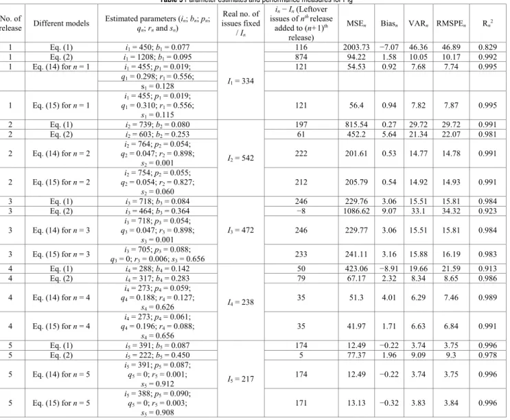
Table 5 Parameter estimates and performance measures for Pig
No. of
release Different models Estimated parameters (qn; rn and sn) in; bn; pn;
Real no. of issues fixed / In in−In (Leftover issues of nth release added to (n+1)th release)
MSEn Biasn VARn RMSPEn Rn2
1 Eq. (1) i1 = 450; b1 = 0.077 I1 = 334 116 2003.73 −7.07 46.36 46.89 0.829 1 Eq. (2) i1 = 1208; b1 = 0.095 874 94.22 1.58 10.05 10.17 0.992 1 Eq. (14) for n = 1 i1 = 455; p1 = 0.019; 121 54.53 0.92 7.68 7.74 0.995 q1 = 0.298; r1 = 0.556; s1 = 0.128 1 Eq. (15) for n = 1 qi11 = 0.310; = 455; p1r = 0.019; 1 = 0.556; s1 = 0.115 121 56.4 0.94 7.82 7.87 0.995 2 Eq. (1) i2 = 739; b2 = 0.080 I2 = 542 197 815.54 0.27 29.72 29.72 0.991 2 Eq. (2) i2 = 603; b2 = 0.253 61 452.2 5.64 21.34 22.07 0.981 2 Eq. (14) for n = 2 qi22 = 0.047; = 764; p2r = 0.054; 2 = 0.898; s2 = 0.001 222 201.61 0.53 14.77 14.78 0.991 2 Eq. (15) for n = 2 qi22 = 0.054; = 754; p2r = 0.055; 2 = 0.827; s2 = 0.060 212 205.79 0.54 14.92 14.93 0.991 3 Eq. (1) i3 = 718; b3 = 0.084 I3 = 472 246 229.76 3.06 15.51 15.81 0.984 3 Eq. (2) i3 = 464; b3 = 0.364 −8 1086.62 9.07 33.1 34.32 0.923 3 Eq. (14) for n = 3 qi33 = 0.047; = 718; p3r = 0.054; 3 = 0.898; s3 = 0.001 246 229.77 3.06 15.51 15.81 0.984 3 Eq. (15) for n = 3 i3 = 705; p3 = 0.088; q3 = 0; r3 = 0.006; s3 = 0.656 233 241.11 3.16 15.88 16.19 0.983 4 Eq. (1) i4 = 288; b4 = 0.142 I4 = 238 50 423.06 −8.91 19.66 21.59 0.913 4 Eq. (2) i4 = 317; b4 = 0.283 79 67.17 2.32 8.34 8.65 0.986 4 Eq. (14) for n = 4 qi44 = 0.188; = 273; p4r = 0.059; 4 = 0.127; s4 = 0.626 35 51.3 4.01 6.29 7.46 0.989 4 Eq. (15) for n = 4 qi44 = 0.196; = 273; p4r = 0.061; 4 = 0.088; s4 = 0.656 35 41.97 1.71 6.63 6.84 0.991 5 Eq. (1) i5 = 391; b5 = 0.087 I5 = 217 174 12.49 −0.22 3.74 3.75 0.996 5 Eq. (2) i5 = 222; b5 = 0.450 5 77.37 1.96 9.09 9.3 0.978 5 Eq. (14) for n = 5 i5q = 391; 5 = 0; rp5 = 0.001; 5 = 0.087; s5 = 0.912 174 12.49 −0.22 3.74 3.75 0.996 5 Eq. (15) for n = 5 i5q = 388; 5 = 0; rp5 = 0.003; 5 = 0.090; s5 = 0.908 171 13.13 −0.32 3.83 3.84 0.996
From Tab. 4, the estimated issues (potential issues) is 364 for case 3 given in Tab. 3 for Release 1. The real number of issues that have been fixed for Release 1 is 332. This implies that 364 – 332 = 32 issues are unresolved and added to Release 2 issue content. The estimated number of issues in Release 2 is (i2 + i1(1 − G1(t1))) = 191. The real
number of issues that have been fixed for Release 2 is 183. This implies that 191 – 183 = 8 issues are unresolved and added to Release 3 issue content. Similarly, 24 issues added to Release 4 from Release 3. In Release 4, 68 issues remained unresolved, and added to the intial issue content of Release 5.
We observed from the results of the proposed entropy based model (case 4 of Tab. 3) that 332 issues have been fixed in Release 1 and the estimated value of the issues is 363. This shows that 363 – 332 = 31 issues are still to be fixed in Release 1 but, they are now added to Release 2
issue content. In Release 2, 183 issues have been fixed and the estimated value for issues is 194 which shows that 11 issues of Release 2 will be now fixed in Release 3. 142 issues have been fixed in Release 4 and the predicted issue is 212, it means 70 issues need to be fixed in Release 4 but they are now added to Release 5.
Similar inference can be drawn for GO and S-shaped models.
We get maximum R2, i.e. 0.99 (in case 3 and case 4);
0.96 (in case 2 and case 3); 0.98 (in case 2, case 3 and case 4); 0.99 (in case 3 and case 4) and 0.98 (in case 3 and case 4) for different releases respectively.
In the proposed models (case 3 and case 4 of Tab. 3), to analyze the rate at which bugs are generated due to NFs and IMPs incorporated, we have taken the average values of p, q, r and s across different releases of a product.
In Avro product, the rates at which new features and feature improvements are incorporated are 0.03 and 0.26. Bugs are generated at the rate of 0.32 and 0.39 due to the addition of NFs and incorporation of IMPs. This shows that the rate of bugs generated due to feature improvements is greater than the rate of bugs generated due to new features incorporation. We get maximum R2 value 0.995 (in case 3
and case 4); 0.99 (in case 1, case 3 and case 4); 0.98 (in case 1, case 3 and case 4); 0.99 (in case 4) and 0.99 (in case
1, case 3 and case 4) for different releases respectively. In Pig product, the rates at which new features and feature improvements incorporated are 0.06 and 0.11. Bugs are generated at the rate of 0.32 and 0.51 due to the addition of NFs and incorporation of IMPs. This shows that the rate of bugs generated due to feature improvements is greater than the rate of bugs generated due to new features incorporation.
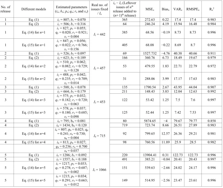
Table 6 Parameter estimates and performance measures for Hive
No. of
release Different models (Estimated parameters in; bn; pn;qn; rn and sn)
Real no. of issues fixed / In in− In (Leftover issues of nth release added to (n+1)th release)
MSEn Biasn VARn RMSPEn Rn2
1 Eq. (1) i1 = 807; b1 = 0.070 I1 = 442 365 272.63 0.22 17.4 17.4 0.983 1 Eq. (2) i1 = 506; b1 = 0.316 64 246.24 4.19 15.94 16.48 0.984 1 Eq. (14) for n=1 qi11 = 0.020; = 827; p1r = 0.055; 1 = 0.921; s1 = 0.004 385 68.56 −0.19 8.73 8.73 0.996 1 Eq. (15) for n=1 qi11 = 0.022; = 847; p1r = 0.056; 1 = 0.766; s1 = 0.156 405 68.08 −0.22 8.69 8.7 0.996 2 Eq. (1) i2 = 526; b2 = 0.097 I2 = 457 69 1527.732 −4.76 40.38 40.66 0.911 2 Eq. (2) i2 = 623; b2 = 0.189 166 360.76 6.73 18.49 19.67 0.979 2 Eq. (14) for n=2 qi22 = 0.082; = 510; p2r = 0.062; 2 = 0.729; s2 = 0.128 53 479.55 1.83 22.71 22.79 0.972 2 Eq. (15) for n=2 qi22 = 0.235; = 488; p2r = 0.042; 2 = 0.709; s2 = 0.014 31 288.06 3.99 17.17 17.63 0.983 3 Eq. (1) i3 = 588; b3 = 0.078 I3 = 453 135 1790.54 2.67 43.95 44.04 0.907 3 Eq. (2) i3 = 664; b3 = 0.179 211 148.43 3.83 12.04 12.63 0.992 3 Eq. (14) for n=3 qi33 = 0.182; = 575; p3r = 0.032; 3 = 0.720; s3 = 0.063 122 53.42 1.25 7.5 7.6 0.997 3 Eq. (15) for n=3 qi33 = 0.180; = 578; p3r = 0.037; 3 = 0.685; s3 = 0.098 125 52.44 1.25 7.42 7.53 0.997 4 Eq. (1) i4 = 795; b4 = 0.081 I4 = 715 80 5874.65 −4 79.67 79.77 0.858 4 Eq. (2) i4 = 1434; b4 = 0.120 719 723.74 8.66 26.51 27.89 0.983 4 Eq. (14) for n=4 i4 = 807; p= 0.241; r4 = 0.025; q4 = 0.730; 4 s4 = 0.004 92 799.65 12.57 26.36 29.21 0.981 4 Eq. (15) for n=4 i4 = 813; p4 = 0.027; 98 760.56 11.89 25.9 28.5 0.982 q4 = 0.236; r4 = 0.700 s4 = 0.037 5 Eq. (1) i5 = 1286; b5 = 0.092 I5 = 1066 220 13904.41 0.31 122.73 122.73 0.996 5 Eq. (2) i5 = 1557; b5 = 0.188 491 385.21 −0.84 20.41 20.43 0.997 5 Eq. (14) for n=5 qi55 = 1217; = 0.278; pr55 = 0.033; = 0.687; s5 = 0.002 151 539.63 −2.66 24.02 24.17 0.996 5 Eq. (15) for n=5 qi55 = 1215; = 0.291; pr55 = 0.034; = 0.663; s5 = 0.012 149 514.95 −2.56 23.47 23.61 0.996
The maximum R2 value is 0.99 (in case 3 and case 4),
0.98 (in case 4), 0.99 (in case 3 and case 4), 0.98 (in case 2, case 3 and case 4) and 0.99 (in all cases) for different releases respectively.
In Hive product, the rates at which NFs and IMPs are incorporated in the software are 0.04 and 0.16. Bugs are generated at the rate of 0.76 and 0.04 due to addition of NFs and incorporation of IMPs. This shows that the rate of bugs generated due to new features addition is greater than the rate of bugs generated due to feature improvements.
In case of jUDDI, we get maximum R2 value, i.e. 0.97
(in case 3 and case 4), 0.95 (in case 2), 0.87 (in case 4) and 0.96 (in case 3 and case 4) for different releases respectively.
In jUDDI product, the rates at which NFs and IMPs are incorporated are 0.11 and 0.12. Bugs are generated at the rate of 0.33 and 0.24 due to the addition of NFs and incorporation of IMPs. This shows that the rate of bugs generated due to new features addition is greater than the rate of bugs generated due to feature improvements.
In case of Whirr product, we get maximum R2 value,
i.e. 0.99 (in case 3 and case 4), 0.96 (in case 3 and case 4), 0.81(in case 4) and 0.76 (in case 3 and case 4) for different releases respectively.
In Whirr product, the rates at which new features and feature improvements are incorporated are 0.08 and 0.11. Bugs are generated at the rate of 0.29 and 0.32 due to the addition of NFs and incorporation of IMPs. This shows that the rate of bugs generated due to feature improvements is
556 Technical Gazette 27, 2(2020), 550-557
greater than the rate of bugs generated due to new features incorporation.
The proposed models give better performance in terms of R2 for all the cases described in Tab. 3. For all the
releases of every product we have taken maximum R2
across all the four cases defined in Tab. 3. Results show that we have 21 cases of maximum R2 for case 4 (proposed
model), 18 cases of maximum R2 for case 3 (proposed
model), 5 cases of maximum R2 for case 2 and 4 cases of
maximum R2 for case 1 out of total 48 cases of maximum
R2 across all the products and releases. During our
experiment, it has been observed that proposed models based on total issues fixed mentioned in case 4 defined in Tab. 3, give the highest cases of maximum goodness of fit.
5.1 Applications of the Proposed Models
The reliability of a software product is an important performance quality attribute. To meet the enormous and frequent requirements, a software is released frequently. The frequent releases must also meet a predefined reliability level. The model predicts the rate at which NFs and IMPs are introduced in the software and also the bugs generated from these introductions. This information will also help in understanding the growth pattern of the software. Based on the proposed models optimal release time can be determined which will assist the release managers in taking release related decisions based on the number of issues fixed.
6 CONCLUSION
We have developed the first mathematical model for issues prediction based on OSS development paradigms: NFs introduction, IMPs and bugs generated from these additions. We have also extended the proposed model by considering the entropy using information theory based measures. We estimated the potential (over a long run) value of different issues in multiple releases of Avro, Pig, Hive, jUDDI and Whirr products of the Apache project. During experimentation, it has been observed that a proportion of issues which is unresolved in the current release are included to the content of future release. Results show that we have 21 cases of maximum R2 for proposed
entropy based model, 18 cases of maximum R2 for the
proposed time based model, 5 cases of maximum R2 for
S-shaped model and 4 cases of maximum R2 for GO model
out of total 48 cases of maximum R2 across all the products
and releases. Entropy based model proposed in this paper gives maximum cases of maximum R2.
The proposed research work will help managers to evaluate the progress in the software products' reliability. In the future, the proposed work will be extended by using Bio inspired algorithms.
Acknowledgement
The authors acknowledge the support by the SCIENCE & ENGINEERING RESEARCH BOARD (SERB), (a statutory body of the Department of Science & Technology, government of India) under grant number MTR/2019/001564.
7 REFERENCES
[1] Gacek, C. & Arief, B. (2004). The many meanings of open source. IEEE software, 21(1), 34-40.
https://doi.org/10.1109/MS.2004.1259206
[2] Hassan, A. E. (2009). Predicting faults using the complexity of code changes. In Proceedings of the 31st International
Conference on Software Engineering (pp. 78-88). IEEE Computer Society. https://doi.org/10.1109/ICSE.2009.5070510
[3] Chaturvedi, K. K., Kapur, P. K., Anand, S., & Singh, V. B. (2014). Predicting the complexity of code changes using entropy based measures. International Journal of System Assurance Engineering and Management, 5(2), 155-164.
https://doi.org/10.1007/s13198-014-0226-5
[4] Kapur, P. K., Pham, H., Aggarwal, A. G., & Kaur, G. (2012). Two dimensional multi-release software reliability modeling and optimal release planning. IEEE Transactions on Reliability, 61(3), 758-768.
https://doi.org/10.1109/TR.2012.2207531
[5] http://www.apache.org/
[6] Shannon, C. E. (1948). A mathematical theory of communication. Bell system technical journal, 27(3), 379-423. https://doi.org/10.1002/j.1538-7305.1948.tb01338.x
[7] Farr, W. Handbook of Software Reliability Engineering, Lyu, M., R. Editor (1996). chapter Software Reliability Modeling Survey, 71-117, McGraw-Hill, New York, NY. [8] Pham, H. (2006) System Software Reliability. Springer.
https://doi.org/10.1007/1-84628-295-0
[9] Xie, M. (1999). Software Reliability Modeling. World Scientific.
[10] Michlmayr, M., Fitzgerald, B., & Stol, K. J. (2015). Why and how should open source projects adopt time-based releases?.
IEEE Software, (2), 55-63. https://doi.org/10.1109/MS.2015.55
[11] Goel, A. L. & Okumoto, K. (1979). Time-dependent error-detection rate model for software reliability and other performance measures. IEEE transactions on Reliability,
28(3), 206-211. https://doi.org/10.1109/TR.1979.5220566
[12] Yamada, S., Ohba, M., & Osaki, S. (1983). S-shaped reliability growth modeling for software error detection.
IEEE Transactions on reliability, 32(5), 475-484.
https://doi.org/10.1109/TR.1983.5221735
[13] Singh, V. B. & Sharma, M. (2014). Prediction of the complexity of code changes based on number of open bugs, new feature and feature improvement. In 2014 IEEE International Symposium on Software Reliability Engineering Workshops (ISSREW), 478-483.
https://doi.org/10.1109/ISSREW.2014.95
[14] Dai, Y. S., Xie, M., Long, Q., & Ng, S. H. (2007). Uncertainty analysis in software reliability modeling by bayesian analysis with maximum-entropy principle. IEEE Transactions on Software Engineering, (11), 781-795.
https://doi.org/10.1109/TSE.2007.70739
[15] Yue, F., Zhang, G., Su, Z., Lu, Y., & Zhang, T. (2015). Multi-software reliability allocation in multimedia systems with budget constraints using Dempster-Shafer theory and improved differential evolution. Neurocomputing, 169, 13-22. https://doi.org/10.1016/j.neucom.2014.09.103
[16] Peng, R., Li, Y. F., Zhang, J. G., & Li, X. (2015). A risk-reduction approach for optimal software release time determination with the delay incurred cost. International Journal of Systems Science, 46(9), 1628-1637.
https://doi.org/10.1080/00207721.2013.827261
[17] Park, J. & Baik, J. (2015). Improving software reliability prediction through multi-criteria based dynamic model selection and combination. Journal of Systems and Software, 101, 236-244. https://doi.org/10.1016/j.jss.2014.12.029
[18] Yang, J., Liu, Y., Xie, M., & Zhao, M. (2016). Modeling and analysis of reliability of multi-release open source software incorporating both fault detection and correction processes.
https://doi.org/10.1016/j.jss.2016.01.025
[19] Zhang, J., Lu, Y., Yang, S., & Xu, C. (2016). NHPP-based software reliability model considering testing effort and multivariate fault detection rate. Journal of systems engineering and electronics, 27(1), 260-270.
[20] Musa, J. D., Iannino, A., & Okumoto, K (1987). Software Reliability: Measurement, Prediction, Application. McGrawHill, New York.
[21] Tamura, Y. & Yamada, S. (2008). A component-oriented reliability assessment method for open source software.
International Journal of Reliability, Quality and Safety Engineering, 15(01), 33-53.
https://doi.org/10.1142/S0218539308002915
[22] Tamura, Y. & Yamada, S. (2009). Optimisation analysis for reliability assessment based on stochastic differential equation modelling for open source software. International Journal of Systems Science, 40(4), 429-438.
https://doi.org/10.1080/00207720802556245
[23] Singh, V. B., Sharma, M., & Pham, H. (2018). Entropy based software reliability analysis of multi-version open source software. IEEE Transactions on Software Engineering,
44(12), 1207-1223. https://doi.org/10.1109/TSE.2017.2766070
[24] Kapur, P. K., Tandon, A., & Kaur, G. (2010, December). Multi up-gradation software reliability model. In 2010 2nd International Conference on Reliability, Safety and Hazard-Risk-Based Technologies and Physics-of-Failure Methods (ICRESH), 468-474.
https://doi.org/10.1109/ICRESH.2010.5779595
[25] Zhu, M. & Pham, H. (2017). A multi-release software reliability modeling for open source software incorporating dependent fault detection process. Annals of Operations Research, 1-18. https://doi.org/10.1007/s10479-017-2556-6
[26] Gokhale, S. S. & Trivedi, K. S. (1998, November). Log-logistic software reliability growth model. In High-Assurance Systems Engineering Symposium, 1998, Proceedings. Third IEEE International (pp. 34-41). IEEE. [27] Kapur, P. K., Kumar, S., & Garg, R. B. (1999). Contributions
to hardware and software reliability. World Scientific. 3.
https://doi.org/10.1142/4011
[28] Raghuvanshi, K. K., Sharma, M., Tandon, A., & Singh, V. B. (2018, May). Quantitative Quality Assessment of Open Source Software by Considering New Features and Feature Improvements. In International Conference on Computational Science and Its Applications, 412-423. Springer, Cham. https://doi.org/10.1007/978-3-319-95174-4_33
[29] Adewumi, A., Misra, S., & Omoregbe, N. (2013a). A review of models for evaluating quality in open source software.
IERI Procedia, 4, 88-92.
https://doi.org/10.1016/j.ieri.2013.11.014
[30] Adewumi, A., Omoregbe, N., Misra, S., & Fernandez, L. (2013). Quantitative quality model for evaluating open source web applications: case study of repository software.
In 2013 IEEE 16th International Conference on
Computational Science and Engineering (pp. 1207-1213). IEEE. https://doi.org/10.1109/CSE.2013.179
[31] Adewumi, A., Misra, S., & Omoregbe, N. (2015, October). Evaluating open source software quality models against ISO 25010. In 2015 IEEE International Conference on Computer and Information Technology; Ubiquitous Computing and Communications; Dependable, Autonomic and Secure Computing; Pervasive Intelligence and Computing (pp. 872-877). IEEE.
https://doi.org/10.1109/CIT/IUCC/DASC/PICOM.2015.130
[32] Adewumi, A., Misra, S., Omoregbe, N., Crawford, B., & Soto, R. (2016). A systematic literature review of open source software quality assessment models. SpringerPlus,
5(1), 1936. https://doi.org/10.1186/s40064-016-3612-4
[33] Adewumi, A., Misra, S., Omoregbe, N., & Sanz, L. F.
(2019). FOSSES: Framework for open‐source software
evaluation and selection. Software: Practice and Experience,
49(5), 780-812. https://doi.org/10.1002/spe.2682
[34] Sharma, M., Pham, H., & Singh, V. B. (2019). Modeling and analysis of leftover issues and release time planning in multi-release open source software using entropy based measure. Computer Systems Science and Engineering, 34(1), 33-46.
Contact information: Abhishek TANDON, Ass. Prof.,
Shaheed Sukhdev College of Business Studies(SSCBS), University of Delhi, PSP Area IV, Dr. K.N. Katju Marg, Sector 16, Rohini, Delhi –110089
E-mail: [email protected]
Meera SHARMA, Ass. Prof., (Corresponding author) Swami Shraddhanand College,
University of Delhi, Alipur, Delhi – 110036, India E-mail: [email protected]
Madhu KUMARI, Ass. Prof., Delhi College of Arts and Commerce,
University of Delhi, Netaji Nagar, New Delhi-110023, India E-mail: [email protected]
V. B. SINGH, Assoc. Prof., (Corresponding author)
Delhi College of Arts and Commerce,
University of Delhi, Netaji Nagar, New Delhi-110023, India E-mail: [email protected]
![Figure 1 A classification of open source users and developers [1]](https://thumb-us.123doks.com/thumbv2/123dok_us/10231885.2927076/1.892.67.414.791.1131/figure-classification-open-source-users-developers.webp)