ensemble classifiers by Genetic Algorithms
Miguel A. Molina-Cabello1, Cristian Accino1, Ezequiel López-Rubio1, and Karl Thurnhofer-Hemsi1
Department of Computer Languages and Computer Science. University of Málaga. Bulevar Louis Pasteur, 35. 29071 Málaga. Spain.
{miguelangel,ezeqlr,karlkhader}@lcc.uma.es, [email protected],
WWW home page:http://www.lcc.uma.es/˜ezeqlr/index-en.html
Abstract. Breast cancer exhibits a high mortality rate and it is the most invasive cancer in women. An analysis from histopathological im-ages could predict this disease. In this way, computational image process-ing might support this task. In this work a proposal which employes deep learning convolutional neural networks is presented. Then, an ensemble of networks is considered in order to obtain an enhanced recognition per-formance of the system by the consensus of the networks of the ensemble. Finally, a genetic algorithm is also considered to choose the networks that belong to the ensemble. The proposal has been tested by carrying out several experiments with a set of benchmark images.
Keywords: Breast cancer classification · medical image processing ·
convolutional neural networks.
1
Introduction
Medicine fields are being enhanced by employing digital image processing. These images are obtained in medical test such as X-ray image, ultrasound image and resonance imaging, among others. According to this information, digital image processing facilitates the analysis of the medical images due to an improvement of them by emphasizing the parts where medical staff focus on. In addition, image processing can be used in order to predict a disease. In this way, a system like this kind could detect an illness by processing an image input. In fact, image processing is essential for pathology detection [8,3,12,16].
An example of the application of image processing could be found in blood sample images obtained in laboratory by microscopy. The hematocrit is the percentage occupied by red blood cells in relation to the total blood. Early detection of several diseases, like anemia, can be indicated by a decrease or growth of the hematocrit value. The image processing supports the analysis of blood images by counting the red blood cells. Several model kinds can be used to this purpose [2,7,9]
Among all types of cancer, breast cancer is the most invasive cancer in women and presents a high mortality rate. Histopathological analysis is currently the most widely used method for breast cancer diagnosis. Thus, automatic classifica-tion of histopathological images can help health professionals to diagnose breast cancer more quickly and effectively. A significant breakthrough in this field was the collection of over 7,900 histopathological image samples, which formed the BreakHis dataset [14], as the previous automated histopathology image recog-nition systems had the limitation of working with small datasets. One of the popular kinds of image recognition is based on the visual feature descriptors to identify patterns on the image [14]. On the other hand, the recent deep learning schema can also be applied to detect and classify the desired parts of the image. In this way, convolutional neuronal networks can be applied to this purpose, for example [13]. In that work, a special kind of Convolutional Neural Network (CNN) has been used, namely AlexNet [5]. It has been previously used in a wide range of fields like vehicle classification in traffic videos [10] as well as blood classification [9].
In this work we outperform the reference model from [13]. In addition, in order to enhance the performance of a network, an ensemble might be considered to this task. In this way, several networks provide their output and an improved output can be obtained by the consensus of the networks [10]. Finally, a genetic algorithm is also considered to choose the networks that belong to the ensemble. The paper is structured as follows. Section 2 presents the methodology of the proposal, differentiating between the considered ensemble types and the genetic algorithm to choose the best possible option for the set of networks which com-prise the ensemble. The experiments have been carried out performed in Section 3, where an optimisation parameter values process and the performance of the ensembles are reported. Finally, the conclusions are provided in Section 4.
2
Methodology
In this section we propose our ensemble methodology in order to improve the performance of Convolutional Neural Network (CNN) classifiers. GivenMclasses and N CNNs, i.e. N classifiers to be combined, let yi be the output vector of thei-th CNN, withi∈ {1, ..., N}. That is,yij is the predicted score for thej-th class by the i-th CNN, for j ∈ {1, ..., M}. Then a subset S ⊆ {1, ...N} of the CNNs can be chosen to form an ensemble of classifiers. Four possible ensemble types are considered:
– Maximum ensemble. The final score for a class is given by the maxima of the scores associated to that class:
zM ax= max{yi |i∈ S} (1)
– Mean ensemble. The final score for a class is given by the arithmetic mean of the scores associated to that class:
– Median ensemble. The final score for a class is given by the median of the scores associated to that class:
zM edian= median{yi|i∈ S} (3)
– Voting ensemble. The final score for a class is given by the number of times that it ranks the highest among the scores yielded by a CNN:
zV oting = i∈ S |j= arg max k∈{1,...,M}{yik} j∈{1,...,M} (4) where|·|stands for the cardinal of a set.
After the ensemble scores are computed, the predicted class is the one which attains the highest score. In order to choose the best possible option for the set of classifiers S which comprise the ensemble, we propose to use a genetic algorithm. Each individual has a chromosome made ofNbinary variables, which indicate whether a specific CNN belongs to the ensemble. The fitness function is the accuracy of the resulting ensemble, measured over a suitable validation set.
3
Experiments
The carried out experiments apply the optimization of the architecture of the neural network proposed in [13] and the fine-tuning of the parameter configura-tion of the trained model openly provided by the authors on [1]. Furthermore, the proposed ensemble methodology is applied as well as the genetic algorithm. The structure of this section is as follows. First of all, Subsection 3.1 shows the software and hardware that have been used. Then, the tested image dataset is specified in Subsection 3.2. After that, the obtained results from the parameter configuration optimisation process are described in Subsection 3.3. And finally, 3.4 exhibits the ensemble process results.
3.1 Methods
Caffe (Convolutional Architecture for Fast Feature Embedding) [4] is the open source deep learning framework chosen for carrying out the experiments. Written in C++, it is developed by Berkeley AI Research (BAIR)1, as well as
commu-nity contributors. Caffe provides GPU (Graphical Processing Unit) acceleration support with CUDA [11]. This is what really makes Caffe fast, as it takes ad-vantage of the fact that images are floating-point matrices that can usually be processed across several computational nodes. In this way, a powerful enough GPU can dramatically accelerate the training of deep neural networks and even becomes vital in order to complete it in a reasonable time.
BAIR and its open community provide a repository of trained models, called Model Zoo, where there are models for a wide variety of purposes. Some of
1
the most well known networks can be found there, such as AlexNet [6] and GoogleNet [15]. As training a network from scratch is always a time-consuming process, sometimes these pre-trained models are taken as starting point. In cases when the purpose of the pre-trained network have something in common, it may be enough to just train some additional layer to achieve a good performance (sometimes even better than by starting from scratch). This technique is known as transfer learning and it is the reason why this kind of repository is very active and supported.
The architecture of the neural network to be optimised, comprises thirteen layers:
– A data layer that expects a LMDB containing 64x64 images. The batch size for training is set to 100.
– Three successive sequences of a convolutional layer, a pooling layer and a ReLU layer. This is a distinctive characteristic of AlexNet.
– Two fully-connected layers. The last of them, which outputs the class scores, is connected to the last layer, a loss layer withsoftmax activation.
All the experiments have been carried out on a 64-bit Personal Computer with an Intel Core i3 Processor (2x 2.0 GHz), 4 GB RAM, NVIDIA GeForce GT 710 as GPU and standard hardware.
3.2 Dataset
In order to evaluate the proposed methodology, a subset from the BreakHist image dataset has been considered to test the approach. It can be downloaded from its website2 upon request.
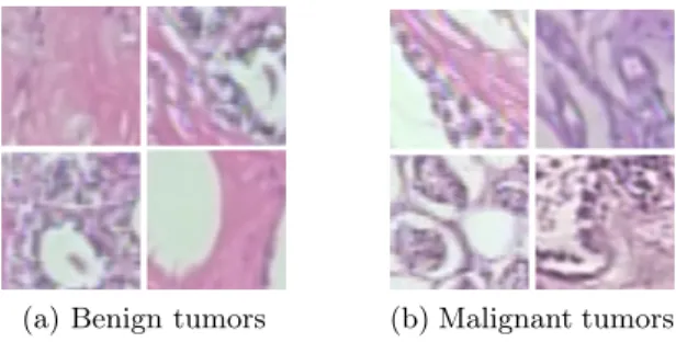
The dataset is composed of the images that were acquired at 40X magni-fication, which consists of 652 benign and 1,370 malignant tumor samples. In addition, we generate 1,000 random 64x64 patches for each image in both sets, as strategy #4 defined in [13] indicates. The resulting dataset is then split into training and test set, which account for 65% and 35%, respectively. Figure 1 exhibits several images from the dataset which show benign and malignant tu-mors.
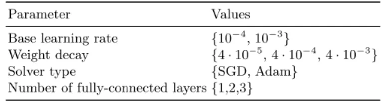
Table 1.Considered parameter values in the CNN optimisation process.
Parameter Values
Base learning rate {10−4,10−3}
Weight decay {4·10−5,4·10−4,4·10−3}
Solver type {SGD, Adam}
Number of fully-connected layers {1,2,3}
2
https://web.inf.ufpr.br/vri/databases/breast-cancer-histopathological-database-breakhis/
(a) Benign tumors (b) Malignant tumors
Fig. 1.64x64 pixel sample patch images used for training the neural networks. They have been generated from random images which belong to the BreakHis dataset. The random patch extraction is already applied on each displayed region. (a) exhibits benign tumors while (b) shows malignant tumors.
3.3 Parameter configuration optimisation process results
In order to compare the performance of the system from a quantitative point of view a well-known measure has been selected: the accuracy (Acc). This measure provides values in the interval[0,1], where higher is better, and represents the percentage of hits of the system, i.e. recognition rate. The definition of this measure can be described as follow:
Acc= T P +T N
T P +F P +F N+T N (5)
where TP is the True positives (number of hits), TN is the True negatives (correct rejections), FN is the False negatives (false alarms) and FP is the False positives (misses).
To quantify our goal, we test the reference model ten times on the test dataset generated. The mean accuracy shown by this model is 0.872±0.015.
The fine-tuning of the parameter configuration is divided into two phases, as it is shown in Figure 2. Each one of this two phases tests the performance of a network by training a network considering different parameters: the first phase tunes the base learning rate and the weight decay, while the second phase tunes the solver type and performs net surgery by either adding or removing a fully-connected layer, so the number of fully-connected layers is also considered. Table 2 exhibits the considered parameter values in this process. The first phase performs the parameter tuning on the reference model and the second one on the model achieving the highest mean accuracy in the first phase, called the first phase candidate model. Finally, the second phase produces the final candidate model, which is the model showing the best performance within such phase.
As training a single network is a quite time-consuming task, the number of iterations is limited to 10,000. Using a batch size of 100 images, there is enough information to extract a tendency of the performance and identify potential candidates.
Fig. 2.CNN optimisation process diagram. Given the reference CNN model, we have tuned several parameter configurations in order to improve the performance of the approach. This process has two different steps: the first one involves the base learning rate and the weight decay, while the second step studies the solver type and the number of fully-connected layers.
Table 2.Considered parameter values in the CNN optimisation process.
Parameter Values
Base learning rate {10−4 ,10−3
}
Weight decay {4·10−5,4·10−4,4·10−3}
Solver type {SGD, Adam}
Number of fully-connected layers {1,2,3}
Besides, 10 models are generated for each configuration so as to reliably mea-sure the performance, since training is not deterministic. Therefore, 60 models are generated at the end of each phase. They will also be useful to apply ensemble learning later on.
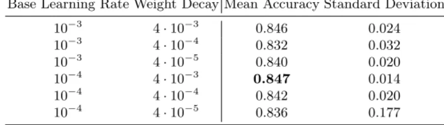
Table 3 gathers all of the combinations tested within the first phase and the performance obtained by each of them in terms of mean accuracy. As it illustrates, a weight decay of 4·10−3 clearly outperforms the rest, while the base learning rates tested do not present any relevant pattern. As a possible explanation of this, we understand that a too lower weight decay does not allow the model to converge fast, since weights can grow too large.
Table 3.Mean accuracy obtained by each parameter configuration tested within the first phase. Best result is highlighted inbold.
Base Learning Rate Weight Decay Mean Accuracy Standard Deviation
10−3 4·10−3 0.846 0.024 10−3 4·10−4 0.832 0.032 10−3 4·10−5 0.840 0.020 10−4 4·10−3 0.847 0.014 10−4 4·10−4 0.842 0.020 10−4 4·10−5 0.836 0.177
For the second phase, the base learning rate and the weight decay are set to
10−4 and4·10−3, respectively, since they showed the best performance in the first phase.
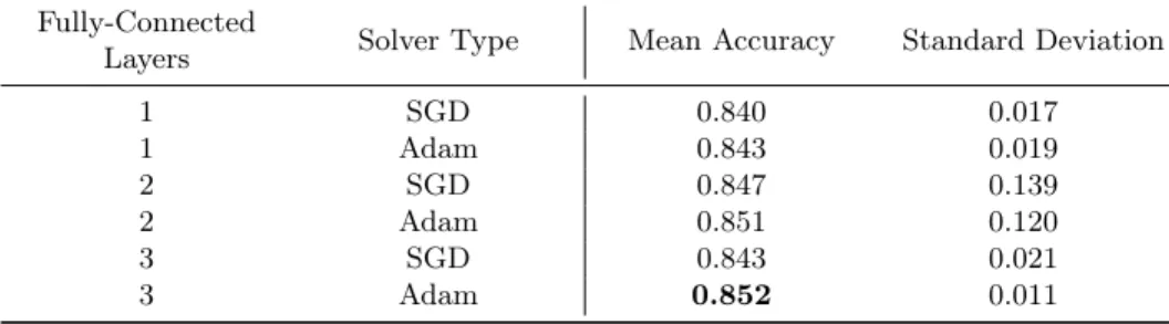
The results obtained throughout the second phase provides more interesting information. Adam solver seems to be more convenient for our dataset, consid-ering that it surpasses SGD for each case. Furthermore, a single fully-connected is not enough to extract rich information, whereas incrementing the number of them does not necessarily means better class scores. Table 6 gathers these results.
Table 4.Mean accuracy obtained by each parameter configuration tested within the second phase. Best result is highlighted inbold.
Fully-Connected
Layers Solver Type Mean Accuracy Standard Deviation
1 SGD 0.840 0.017 1 Adam 0.843 0.019 2 SGD 0.847 0.139 2 Adam 0.851 0.120 3 SGD 0.843 0.021 3 Adam 0.852 0.011
Given the commented results, the final candidate configuration reaches an accuracy of 0.852±0.011 at the 10,000th iteration and consists the parameter values which are shown in Table 5.
Table 5.Considered parameter values after the CNN optimisation process.
Parameter Value
Base learning rate 10−3 Weight decay 4·10−3
Solver type Adam
Number of fully-connected layers 3
Then, we resumed the training for the model with this configuration until the 50,000th iteration. The mean accuracy achieved at the 50,000th is 0.891±
0.020, which surpasses the 0.872±0.015 obtained by the reference model on our test dataset.
3.4 Ensemble process results
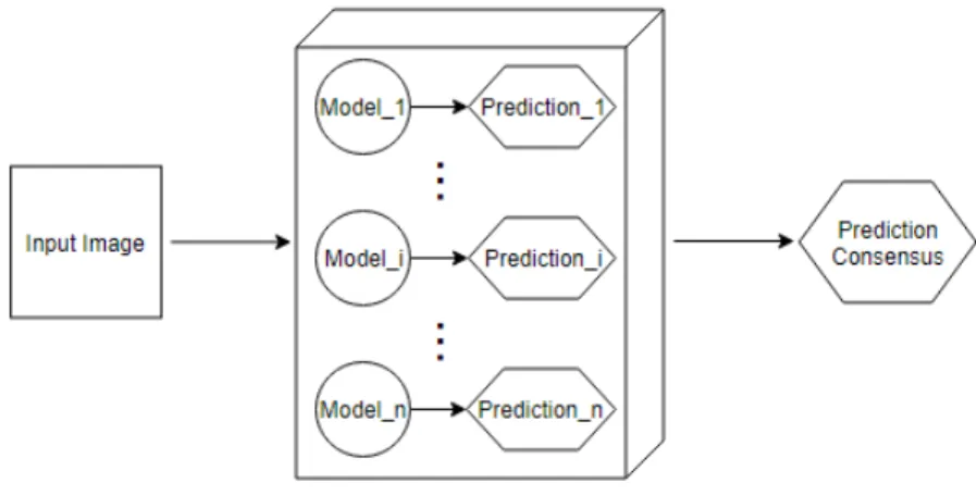
Ensemble learning is a well-known technique used in machine learning to improve robustness over a single estimator. To do that, ensemble methods combine the
predictions of several estimators trained with a given algorithm, as illustrated in Figure 3. In this case, we have considered 30 networks.
Fig. 3. Diagram of an ensemble. It receives an image as input and its output is a consensus on all the predictions generated by each model composing it.
Firstly, we built an voting ensemble comprising the generated neural networks with the final candidate configuration.
In order to measure its performance, we undertook 10 test iterations with a batch size of 100 using the test dataset. Here, each iteration performs a step forward on a model, which computes the class scores for each picture in the batch, and outputs the accuracy achieved on the batch.
The ensembles, with a mean accuracy of 0.863±0.037, outperforms the mean accuracy obtained by a single model, 0.851±0.033. This single model is the one within the ensemble that achieved the best performance in the second phase of the hyperparameter optimisation carried out. Besides, the ensemble shows higher performance at the vast majority of test iterations. However, these accuracy values are lower than those obtained in the second phase. This is basically due to the test images used this time, since the reference model reaches a lower mean accuracy value as well, 0.824±0.047. Therefore, the ensemble represents a performance improvement of 4% over the reference model.
As it seems to be worthwile to apply ensemble learning, we now apply the genetic algorithm proposed in our methodology. In order to do so, we run the evolution of a population of 300 individuals over 1000 generations. Each indi-vidual is an array of 30 boolean elements. A value of 0 means that the neural network represented by the element is left out of the ensemble, whereas a value of 1 includes the neural network within the ensemble. The fitness function is the testing process previously mentioned, which measures the performance of the ensemble that the individual represents. Therefore, the fitness value of each element is the mean accuracy achieved by the ensemble of neural networks being
represented. The aim of the evolution is to maximise the fitness value, whose maximum value is 1. If an individual reached such performance, the evolution would stop.
The first generation starts with 300 individuals generated randomly and each generation undertakes the following actions:
– At the beginning, each pair of individuals within the population may be crossed over with a probability of 0.5.
– Within a generation, each individual may mutate by flipping some of its elements with a probability of 0.2.
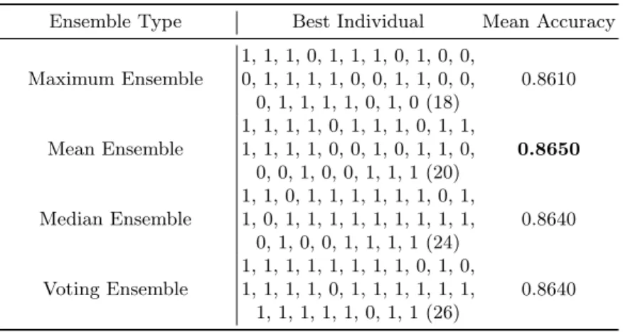
– At the end of each a generation, each evolved individual is evaluated by the fitness function. The next generation starts with the resulting individuals. The performance of all of the ensemble types considered are shown in Table 6. As it can be observed, Mean Ensemble obtains the best performance of the considered ensembles. However, the performance is very similar among them.
Table 6. Best individual after the evolution for each type of ensemble and its mean accuracy achieved. The ones mean the presence of the i-th network in the ensemble whereas the zeros mean the abscence (the number of used networks in the ensemble is shown within the brackets). Best result is highlighted inbold.
Ensemble Type Best Individual Mean Accuracy Maximum Ensemble 1, 1, 1, 0, 1, 1, 1, 0, 1, 0, 0, 0, 1, 1, 1, 1, 0, 0, 1, 1, 0, 0, 0, 1, 1, 1, 1, 0, 1, 0 (18) 0.8610 Mean Ensemble 1, 1, 1, 1, 0, 1, 1, 1, 0, 1, 1, 1, 1, 1, 1, 0, 0, 1, 0, 1, 1, 0, 0, 0, 1, 0, 0, 1, 1, 1 (20) 0.8650 Median Ensemble 1, 1, 0, 1, 1, 1, 1, 1, 1, 0, 1, 1, 0, 1, 1, 1, 1, 1, 1, 1, 1, 1, 0, 1, 0, 0, 1, 1, 1, 1 (24) 0.8640 Voting Ensemble 1, 1, 1, 1, 1, 1, 1, 1, 0, 1, 0, 1, 1, 1, 1, 0, 1, 1, 1, 1, 1, 1, 1, 1, 1, 1, 1, 0, 1, 1 (26) 0.8640
The most significant result is the number of network that the best of each ensemble types uses. The Maximum and Mean ensembles have into account only 18 and 20 networks from the 30 available ones. Nevertheless, the Median and Voting ensembles employ a higher number of the available networks. Thus, a lower computational and memory costs is achieved with the two first approaches.
4
Conclusion
An approach for the detection of breast cancer by using histopathological images has been presented in this work. This proposal is based on the use of the deep
convolutional neural networks, in particular the Alexnet model. Given a model as a base, a two-phase process to optimise the parameter values has been proposed. According to the exhibited results, a not very low weight decay outperforms other higher considered options, while the tested base learning rates do not present any relevant pattern. In addition, Adam solver type works better than SGD type. Furthermore, the more fully-connected layers the architecture employes a higher performance is yielded.
Moreover, several ensemble types have been considered in order to enhance the performance of the system. A genetic algorithm is also applied to improve it. Although the different tested ensemble types provide a similar performance, Maximum and Mean ensembles employ a lower number of networks, so that, they need a lower memory and computational requirements. The obtained results indicate that the presented proposal is suitable to classify breast cancer images correctly with a high efficiency.
Acknowledgments
This work is partially supported by the Ministry of Economy and Competitive-ness of Spain under grant TIN2014-53465-R, project name Video surveillance by active search of anomalous events and TIN2016-75097-P. It is also partially supported by the Autonomous Government of Andalusia (Spain) under projects TIC-6213, project name Development of Self-Organizing Neural Networks for Information Technologies; and TIC-657, project name Self-organizing systems and robust estimators for video surveillance. All of them include funds from the European Regional Development Fund (ERDF). The authors thankfully ac-knowledge the computer resources, technical expertise and assistance provided by the SCBI (Supercomputing and Bioinformatics) center of the University of Málaga. They also gratefully acknowledge the support of NVIDIA Corporation with the donation of two Titan X GPUs used for this research. The authors would like to thank the grant of the Universidad de Málaga.
References
1. Caffe models trained on the images of breakhist acquired with 40x magnification factor. https://web.inf.ufpr.br/vri/databases/ breast-cancer-histopathological-database-breakhis/. Accessed: 2017-05-25
2. Bagui, O.K., Zoueu, J.T.: Red blood cells counting by circular hough transform using multispectral images. Journal of Applied Sciences14(24), 3591–3594 (2014) 3. Davis, R., Boyers, S.: The role of digital image analysis in reproductive biology and
medicine. Archives of pathology & laboratory medicine116(4), 351–363 (1992) 4. Jia, Y., Shelhamer, E., Donahue, J., Karayev, S., Long, J., Girshick, R.,
Guadar-rama, S., Darrell, T.: Caffe: Convolutional architecture for fast feature embedding. In: MM 2014 - Proceedings of the 2014 ACM Conference on Multimedia, pp. 675– 678 (2014)
5. Krizhevsky, A., Sutskever, I., Hinton, G.: ImageNet classification with deep con-volutional neural networks. Advances in Neural Information Processing Systems
25, 1097–1105 (2012)
6. Krizhevsky, A., Sutskever, I., Hinton, G.E.: Imagenet classification with deep con-volutional neural networks. In: Advances in Neural Information Processing Sys-tems, vol. 2, pp. 1097–1105 (2012)
7. Mazalan, S.M., Mahmood, N.H., Razak, M.A.A.: Automated red blood cells count-ing in peripheral blood smear image uscount-ing circular hough transform. In: Artificial Intelligence, Modelling and Simulation (AIMS), 2013 1st International Conference on, pp. 320–324. IEEE (2013)
8. McAuliffe, M.J., Lalonde, F.M., McGarry, D., Gandler, W., Csaky, K., Trus, B.L.: Medical image processing, analysis and visualization in clinical research. In: Computer-Based Medical Systems, 2001. CBMS 2001. Proceedings. 14th IEEE Symposium on, pp. 381–386. IEEE (2001)
9. Molina-Cabello, M.A., López-Rubio, E., Luque-Baena, R.M., Rodríguez-Espinosa, M.J., Thurnhofer-Hemsi, K.: Blood cell classification using the hough transform and convolutional neural networks. In: World Conference on Information Systems and Technologies, pp. 669–678. Springer (2018)
10. Molina-Cabello, M.A., Luque-Baena, R.M., López-Rubio, E., Thurnhofer-Hemsi, K.: Vehicle type detection by ensembles of convolutional neural networks operating on super resolved images. Integrated Computer-Aided Engineering (Preprint), 1– 13 (2018)
11. Nickolls, J., Buck, I., Garland, M., Skadron, K.: Scalable parallel programming with cuda. Queue 6(2), 40–53 (2008). https://doi.org/10.1145/1365490.1365500. URLhttp://doi.acm.org/10.1145/1365490.1365500
12. Nogueira, P.A., Teófilo, L.F.: A multi-layered segmentation method for nucleus detection in highly clustered microscopy imaging: a practical application and vali-dation using human u2os cytoplasm–nucleus translocation images. Artificial Intel-ligence Review42(3), 331–346 (2014)
13. Spanhol, F.A., Oliveira, L.S., Petitjean, C., Heutte, L.: Breast cancer histopatho-logical image classification using convolutional neural network. In: International Joint Conference on Neural Networks (IJCNN 2016) Vancouver, Canada, p. 2560–2567 (2016)
14. Spanhol, F.A., Oliveira, L.S., Petitjean, C., Heutte, L.: A dataset for breast cancer histopathological image classification. IEEE Transactions on Biomedical Engineer-ing 63(7), 1455–1462 (2016)
15. Szegedy, C., Liu, W., Jia, Y., Sermanet, P., Reed, S., Anguelov, D., Erhan, D., Vanhoucke, V., Rabinovich, A.: Going deeper with convolutions. In: Computer Vision and Pattern Recognition (CVPR) (2015). URL http://arxiv.org/abs/ 1409.4842
16. Vishnuvarthanan, A., Rajasekaran, M.P., Govindaraj, V., Zhang, Y., Thiyagara-jan, A.: Development of a combinational framework to concurrently perform tissue segmentation and tumor identification in t1-w, t2-w, flair and mpr type magnetic resonance brain images. Expert Systems with Applications95, 280–311 (2018)