Prediction of Cardiovascular Events Using Heart Rate Variability and Stroke Volume Variability

(1)

PREDICTION OF CARDIOVASCULAR EVENTS USING HEART RATE VARIABILITY AND

STROKE VOLUME VARIABILITY

By

NISHIGANDHA KALE

Bachelor of Engineering in Electronics and Telecommunication Engineering

Pune University Pune, India

2011

Submitted to the Faculty of the Graduate College of the Oklahoma State University

in partial fulfillment of the requirements for

the Degree of MASTER OF SCIENCE

(2)

ii

PREDICTION OF CARDIOVASCULAR EVENTS USING HEART RATE VARIABILITY AND

STROKE VOLUME VARIABILITY

Thesis Approved: Dr. Johnson Thomas Thesis Adviser Dr. Johnson Thomas Dr. David Cline Dr. Bruce Benjamin

(3)

iii

Acknowledgements reflect the views of the author and are not endorsed by committee members or Oklahoma State University.

ACKNOWLEDGEMENTS

The Master’s degree from the Computer Science department, Oklahoma State University has given me immense experience and knowledge in my field of interest. I would like to thank my thesis advisor, Dr. Johnson Thomas for his continuous assistance and encouragement when I was doing my research.

I would like to express my gratitude to my committee members, Dr. Bruce Benjamin and Dr. David Cline for their guidance and support. I would also like to extend my thanks to Dr. Anthony Alfrey for helping us in classifying patients into groups.

Finally, I wish to express my profound gratitude to my family and friends who supported me throughout my years of study.

(4)

iv Name: NISHIGANDHA KALE

Date of Degree: JULY, 2018

Title of Study: PREDICTION OF CARDIOVASCULAR EVENTS USING HEART RATE VARIABILITY AND STROKE VOLUME VARIABILITY

Major Field: COMPUTER SCIENCE Abstract:

Many firefighters die of heart attacks while on duty or even after they have left the profession because of the stress their job puts on their body. Heart attacks were the primary reason of active firefighters’ death. Given that other fields like the military and police have similar high levels of stress at work, it is more likely that those who work in these fields are also susceptible to heart attacks. This calls for close monitoring of the heart condition of such people working in highly stressful environments.

Currently, there are many ways to monitor and measure the health of a heart. One way is to measure the state of the heart is by analyzing heart rate variability (HRV) and Stroke Volume Variability (SVV). Although our long-term goal is to develop a Fire Rescue network to identify on duty firefighters at risk, our preliminary work has focused on people from all walks of life. The first step is to analyze heart rate variability signals of healthy and unhealthy patients to predict a cardiac event with the best sensitivity and specificity. Using machine learning algorithms, we can predict a patient’s heart health using Heart Rate Variability (HRV) and Stroke Volume Variability (SVV). Heart Rate Variability (HRV) is different for a human in different postures and physical conditions. Our study also focuses on Heart Rate Variability (HRV) analysis of patient’s data while they are sitting and lying because patients’ health can be predicted using machine learning algorithms on heart data collected in different postures.

Our result showed that both HRV and SVV analysis predictor variables on the random forest model produces better sensitivity and specificity. Results showed that a distinction could be made using machine learning techniques between postures, healthy and unhealthy people by analyzing HRV and SVV signals.

Keywords: Cardiovascular, Heart Rate Variability, Stroke Volume Variability, Posture Analysis, Random Forest, Sensitivity, Specificity

(5)

v

TABLE OF CONTENTS

Chapter Page

I. INTRODUCTION ...1

II. CARDIOVASCULAR SYSTEM ...4

2.1 Cardiovascular System...4

2.1.1 Circulatory of Cardiovascular System ...4

2.1.1.1 Oxygenated blood fills the left ventricle ...7

2.1.1.2 Blood is ejected from the left ventricle into the aorta ...7

2.1.1.3 Cardiac output is distributed among various organs ...7

2.1.1.4 Blood flow from the organs is collected in the veins ...8

2.1.1.5 Venous return to the right atrium ...8

2.1.1.6 Mixed venous blood fills the right ventricle ...9

2.1.1.7 Blood is ejected from the right ventricle into the pulmonary artery ...9

2.1.1.8 Blood flow from the lungs is returned to the heart via the pulmonary vein ...9

2.1.2 Pressures in the Cardiovascular System ...9

2.1.3 Arterial Pressure in the Systemic Circulation ...10

2.1.3.1 Diastolic Pressure ...10

2.1.3.2 Systolic Pressure ...11

2.1.3.3 Pulse Pressure ...11

2.2 Heart Rate Variability ...11

2.3 Stroke Volume Variability ...13

2.3.1 Stroke Volume ...14

2.3.2 Cardiac Output ...14

III. REVIEW OF LITERATURE ...15

3.1 Related Work ...15

IV. PROBLEM STATEMENT ...17

4.1 Problem Specification ...17

4.2 Proposed Solution ...17

4.2.1 Part 1- Prediction of cardiovascular events using HRV of healthy and unhealthy patients...18

4.2.1.1 Input Data...18

4.2.1.1.1 Smart Health for Assessing the Risk of Events via ECG Database ...18

(6)

vi

4.2.1.2 Methodology ...19

4.2.1.3 Results and Analysis ...19

4.2.1.3.1 Prediction Analysis Results with Data Filtering ...21

4.2.1.3.2 Prediction Analysis Results without Data Filtering ...22

4.2.1.4 Conclusion ...25

4.2.2 Part 2- Heart Rate Variability (HRV) and Stroke Volume Variability (SVV) analysis of patient’s according to their posture ...26

4.2.2.1 Input Data...26

4.2.2.1.1 The EUROBAVAR data set ...26

4.2.2.2.1 ABP Beat Detection ...26

4.2.2.2.2 ABP Feature Selection ...27

4.2.2.2.3 Feature Statistics Calculation ...28

4.2.2.3.1 Prediction Analysis Results with HRV and SVV analysis ...30

4.2.3 Part 3- Prediction of cardiovascular events using HRV and SVV of healthy and unhealthy patients. ...32

4.2.3.1 Input Data...33

4.2.3.1.1 The MGH/MF Waveform Database ...33

4.2.3.1.2 The EUROBAVAR data set ...33

4.2.3.2.1 ECG and ABP Signal Extraction ...33

4.2.3.2.2 Extract RR intervals for HRV analysis ...35

4.2.3.2.3 ABP Beat Detection ...36

4.2.3.2.4 ABP Feature Selection ...37

4.2.3.2.5 Feature Statistics Calculation ...37

4.2.3.2.6 Patients Classification ...38

4.2.3.2.7 Prediction Model ...38

4.2.3.3.1 Prediction Analysis Results with HRV analysis only...41

4.2.3.3.2 Prediction Analysis Results with HRV and SVV analysis ...43

4.2.3.3.3 Prediction Analysis Results with SVV analysis ...45

4.2.3.3.4 Prediction Analysis Results with SVV analysis with Pulse Pressure Standard Deviation as a predictor variable ...47

4.2.3.3.5 Prediction Analysis Results with Combination of HRV and SVV ...49

(7)

vii

4.2.3.3.6 Prediction of Gender with HRV and

SVV analysis ...51

4.2.3.3.7 Prediction of Age with HRV and SVV analysis ...54

4.3 Proposed System Architecture ...57

V. CONCLUSION ...59

REFERENCES ...62

(8)

viii

LIST OF TABLES

Table Page

1. Cardiovascular Responses to Exercise ...13

2. Terminologies ...20

3. Actual and Predicted result for Cardiovascular Events with Data Filtering ...22

4. Actual and Predicted result for Cardiovascular Events without Data Filtering ...23

5. t-test Results ...25

6. Actual and Predicted result for lying and sitting Patients with HRV and SVV analysis ...31

7. Min Max Accuracy and MAPE for posture analysis ...32

8. Actual and Predicted result for Healthy and Unhealthy Patients with HRV analysis ...42

9. Min Max Accuracy and MAPE for healthy and unhealthy patients with HRV analysis ...43

10. Actual and Predicted result for healthy and unhealthy patients with HRV and SVV analysis ...45

11. Min Max Accuracy and MAPE for healthy and unhealthy patients with HRV and SVV analysis ...45

12. Actual and Predicted result for Healthy and Unhealthy Patients with HRV and SVV analysis ...47

(9)

ix

13. Min Max Accuracy and MAPE for healthy and unhealthy

patients with SVV analysis ...47 14. Actual and Predicted result for Healthy and Unhealthy

Patients with HRV and SVV analysis ...49 15. Min Max Accuracy and MAPE for healthy and unhealthy

patients with SVV analysis ...49 16. Actual and Predicted result of gender with HRV and SVV analysis ...53 17. Min Max Accuracy and MAPE for healthy and unhealthy

patients with SVV analysis ...54 18. Actual and Predicted result of age with HRV and SVV analysis ...56 19. Min Max Accuracy and MAPE for healthy and unhealthy

(10)

x

LIST OF FIGURES

Figure Page

1. Heart Chambers and Valves ...5

2. Circuitry of The Cardiovascular System...6

3. Systemic arterial pressure during the cardiac cycle ...10

4. Heart Rate variability ...13

5(a). SDNN with Data Filtering ...21

5(b). SDNN_without Data Filtering ...21

6(a). MeanRR with Data Filtering ...21

6(b). MeanRR without Data Filtering ...21

7(a). DFA Scaling Component with Data Filtering ...24

7(b). DFA Scaling Component without Data Filtering ...24

8. Slope sum function ...27

9(a). MeanRR of Lying and Sitting Patients ...28

9(b). SDRR of Lying and Sitting Patients ...28

10(a). Mean Systolic Pressure of Lying and Sitting Patients...29

10(b). SD Systolic Pressure of Lying and Sitting Patients ...29

11(a). Mean Diastolic Pressure of Lying and Sitting Patients ...29

(11)

xi

12. VarImpPlot for posture analysis ...31

13. Slope sum function ...37

14(a). Mean Systolic Pressure of Healthy and Unhealthy Patients ...39

14(b). Mean Diastolic Pressure of Healthy and Unhealthy Patients ...39

15(a). Standard Deviation of Systolic Pressure of Healthy and Unhealthy Patients ...39

15(b). Standard Deviation of Diastolic Pressure of Healthy and Unhealthy Patients .39 16. Mean Pulse Pressure of Healthy and Unhealthy Patients ...40

17(a). RRMean of Healthy and Unhealthy Patients...40

17(b). Standard Deviation of RR of Healthy and Unhealthy Patients ...40

18. Standard Deviation of Pulse Pressure of Healthy and Unhealthy Patients ...40

19. VarImpPlot for healthy and unhealthy patients with HRV analysis. ...42

20. VarImpPlot for healthy and unhealthy patients with HRV and SVV analysis ...44

21. VarImpPlot for healthy and unhealthy patients with SVV analysis ...46

22. VarImpPlot for healthy and unhealthy patients with Standard Deviation of Pulse Pressure and SVV analysis ...48

23. Min-Max Accuracy and MAPE for Combination of HRV and SVV analysis ...50

24. Variability Plot of Healthy and Unhealthy People ...51

25. VarImpPlot for gender analysis ...53

26. VarImpPlot for age analysis...55

(12)

1

CHAPTER I

INTRODUCTION

The heart is a powerful organ that requires a constant flow of oxygen rich blood to nourish it. When that flow of blood is severely reduced or cut off completely, the heart loses its supply of oxygen and the heart muscle becomes damaged or dies. This event is called a heart attack or a myocardial infarction [1]. There are several risk factors that make a person more likely to have a heart attack. Some common risk factors are smoking, high cholesterol, and obesity. Stress is also a risk factor that greatly increases one’s chances of having a heart attack [2]. This, of course, is important because many jobs cause a great amount of stress that can lead to people having more heart attacks. As an example, firefighters deal with many life-threatening situations throughout their careers. They are expected to deal with high stress situations and exert sustained physical effort for extended periods of time, all without concern for their own safety. Consequently, many firefighters die of heart attacks while on duty or even after they have left the profession because of the stress their job puts on their body. The National Fire Protection Association found that 59 percent of on duty deaths in 2015 were due to stress and medical reasons. 51 percent of these on duty deaths were sudden cardiac deaths [3]. Thus, heart attacks were the primary reason of active firefighters’ death. Given that other fields like the military and police have similar high levels of stress at work, it is more likely that those who work in these fields

(13)

2

are susceptible to heart attacks. This calls for close monitoring of heart condition of on duty servicemen like firefighters, military personnel, and police officers.

Currently, there are many ways to monitor and measure the health of a heart. One such tool to measure the state of the heart is known as heart rate variability (HRV). Although our long-term goal is to develop a Fire Rescue network to identify on duty firefighters at risk, our preliminary work has focused on people from all walks of life. The first step is to analyze heart rate variability signals of healthy and unhealthy patients to predict when a cardiac event will occur with the best sensitivity and specificity. Using machine learning algorithms, we can predict a patient’s heart health using Heart Rate Variability (HRV) and Stroke Volume Variability (SVV). In our preliminary work we used the Random Forest algorithm as the classifier to classify healthy and unhealthy patients. Our results showed that data filtering on the random forest model produces the best sensitivity and specificity. Our next goal is to analyze stroke volume variability because we can predict a patient’s heart health using both HRV and SVV with the best sensitivity and specificity.

Heart Rate Variability (HRV) is different for a human in different postures and physical conditions. For example, a person heart rate variability while lying in bed will be different from heart rate variability while sitting. Our study also focuses on Heart Rate Variability (HRV) analysis of a patient’s data while they are sitting and lying because patients’ health can be predicted using machine learning algorithms on heart data collected in different postures.

(14)

3

In chapter II we describe the essential functioning of the cardiovascular system. Chapter III presents a literature review on work done on heart rate variability and stroke volume variability. In chapter IV we present the problem statement, proposed solution and system architecture. The results are also presented and discussed. In chapter V we have describe our findings and conclusion.

(15)

4

CHAPTER II

CARDIOVASCULAR SYSTEM

2.1 Cardiovascular System

The main function of the cardiovascular system is to deliver nourished blood to tissues. The heart contracts to generate pressure to pump nourished blood through a series of blood vessels [10]. There are two types of blood vessels, Arteries and Veins. The arteries carry blood from the heart to the tissues and the veins carry blood from the tissues to the heart.

The cardiovascular system [10] is involved in numerous homeostatic functions.

▪ Regulate arterial blood pressure

▪ Deliver regulatory hormones (from the endocrine glands to target tissues)

▪ Regulate body temperature

▪ Homeostatic adjustments to changed physiologic states e.g. exercise, hemorrhage, and changes in posture.

2.1.1 Circulatory of Cardiovascular System [10]

The below figure shows the schematic diagram of the circuitry of the cardiovascular system [10]. There are two chambers in each side of heart, an atrium and a ventricle. The Atrium

(16)

5

and Ventricle are connected by one-way valves known as atrioventricular (AV) valves. Blood can flow only in one direction, from the atrium to the ventricle, through AV valves [10].

Figure 1. Heart Chambers and Valves [24]

The Left and right sections of the heart have different functions. The left heart and the systemic arteries, capillaries, and veins are known as systemic circulation [10]. The left ventricle pumps blood to all organs of the body except the lungs. The right heart and the pulmonary arteries, capillaries, and veins are known as pulmonary circulation [10]. The right ventricle pumps blood to the lungs. The left heart and right heart function in series so that blood is pumped sequentially from the left heart to the systemic circulation, to the right heart, to the pulmonary circulation, and then back to the left heart [10].

The rate at which blood is pumped from one of the ventricle is known as cardiac output. Because the two sides of the heart operate in series, the cardiac output of the left ventricle is the same as the cardiac output of the right ventricle in the steady state [10]. The rate at

(17)

6

which blood is returned to the atria from the veins is called the venous return [10]. Venous return to the left heart equals venous return to the right heart in the steady state because the left heart and the right heart operate in sequence. Therefore, in the steady state, cardiac output from the heart is the same as venous return to the heart. The steps involved in one complete cycle through the cardiovascular system are shown in Figure 1. The circled numbers in the figure correspond to the steps described below.

(18)

7

2.1.1.1 Oxygenated blood fills the left ventricle

Oxygenated blood from the lungs returns to the left atrium via the pulmonary vein. This blood then flows from the left atrium to the left ventricle through the mitral valve (the AV valve of the left heart).

2.1.1.2 Blood is ejected from the left ventricle into the aorta

When the left ventricle contracts oxygenated blood goes from the left ventricle to aorta through the aortic valve (the semilunar valve of the left side of the heart), which is located between the left ventricle and the aorta. As mentioned earlier, the amount of blood ejected from the left ventricle per unit time is called the cardiac output. Oxygenated blood then flows through the arterial system, driven by the pressure created by contraction of the left ventricle.

2.1.1.3 Cardiac output is distributed among various organs

The total cardiac output of the left heart is distributed among the organ systems via sets of parallel arteries. So, simultaneously, 15% of the cardiac output is delivered to the brain through the cerebral arteries, 5% is delivered to the heart through the coronary arteries, 25% is delivered to the kidneys through the renal arteries, and so forth. The percentage distribution of cardiac output among the various organ systems is not fixed, however. For example, during intense exercise, the percentage of the cardiac output going to skeletal muscle increases, compared with the percentage at rest.

(19)

8

There are three major mechanisms for achieving such a change in blood flow to an organ system. In the first mechanism, the cardiac output remains constant, but the blood flow is redistributed among the organ systems by the selective alteration of arteriolar resistance. In this case, blood flow to one organ can be increased at the expense of blood flow to other organs.

In the second mechanism, the cardiac output increases or decreases, but the percentage distribution of blood flow among the organ systems is kept constant.

The third scenario is a combination of the first two mechanisms where cardiac output and the percentage distribution of blood flow are changed.

2.1.1.4 Blood flow from the organs is collected in the veins

The blood leaving the organs is venous blood and contains waste products from metabolism, such as carbon dioxide (CO2). Venous blood is collected in veins of increasing size and finally in the largest vein, the vena cava that carries venous blood to the right heart.

2.1.1.5 Venous return to the right atrium

The right atrium fills with venous blood because of higher pressure in the vena cava than the right atrium. In the steady state, venous return to the right atrium equals cardiac output from the left ventricle.

(20)

9

2.1.1.6 Mixed venous blood fills the right ventricle

Mixed venous blood flows from the right atrium to the right ventricle through the AV valve in the right heart, the tricuspid valve.

2.1.1.7 Blood is ejected from the right ventricle into the pulmonary artery

When the right ventricle contracts, blood is ejected through the pulmonic valve (the semilunar valve of the right side of the heart) into the pulmonary artery, which carries blood to the lungs. The cardiac output ejected from the right ventricle is identical to the cardiac output that was ejected from the left ventricle. In the capillary beds of the lungs, oxygen(O2) is added to the blood from alveolar gas, and CO2 is removed from the blood and added to the alveolar gas.

2.1.1.8 Blood flow from the lungs is returned to the heart via the pulmonary vein Oxygenated blood is supplied back to the left atrium via the pulmonary vein to begin a new cardiac cycle.

2.1.2 Pressures in the Cardiovascular System

Blood Pressure is not the same throughout the cardiovascular system. In the cardiovascular system the blood flows because of the pressure difference between the heart and blood vessels [10]. The principle of blood flow in the cardiovascular system is known as hemodynamics [10].

(21)

10

2.1.3 Arterial Pressure in the Systemic Circulation

Even though mean pressure in the arteries is high and constant, there are oscillations or pulsations of arterial pressure. These pulsations reflect the pulsatile activity of the heart: ejecting blood during systole, resting during diastole, ejecting blood, resting, and so forth. Each cycle of pulsation in the arteries coincides with one cardiac cycle [10].

The below figure 2 shows prolonged version of two such pulsations in a large artery.

Figure 3. Systemic arterial pressure during the cardiac cycle [10]

2.1.3.1 Diastolic Pressure

It is the lowest arterial pressure measured during a cardiac cycle and is the pressure in the arteries during ventricular relaxation when no blood is pushed from the left ventricle.

(22)

11

2.1.3.2 Systolic Pressure

It is the highest arterial pressure measured during a cardiac cycle. It is the pressure in the arteries after blood is pushed from the left ventricle during systole.

2.1.3.3 Pulse Pressure

It is the difference between systolic pressure and diastolic pressure.

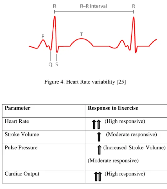
2.2 Heart Rate Variability (HRV)

HRV looks at the variation between each heartbeat. Heart Rate Variability is measured by calculating the variation between heartbeats (RR intervals) within a specific timeframe. A normal healthy heart does not beat at a regular pace but rather is influenced by many factors such as exercise, stress, respiration, and circadian rhythms. For example, increase in physical activity/exercise would increase the heart rate and subsequently lead to an increase in HRV [4]. Table 1 [10] shows the cardiovascular responses to exercise. This variation is caused by the sympathetic and parasympathetic nervous systems of the body. The sympathetic system works to increase heart rate while the parasympathetic system decreases the heart rate [5]. Thus, a decrease in HRV suggests that the sympathetic and parasympathetic nervous systems are not able to change the heart rate very much. This decreased HRV due to a decreased adaptive nervous system is thought to be associated with increased morbidity [6]. Therefore, a healthy heart is considered to have more variation while a less healthy heart would have low HRV. Studies analyzing HRV have found that low HRV is associated with premature heart attack, an increased risk of coronary

(23)

12

heart disease, and the development of a stroke in a healthy subject [7]. Other studies found the same strong association between low HRV and cardiovascular disease and even an association with low HRV and death caused by cancer [8]. Given the importance of low HRV, there have been many attempts to use HRV to predict when a cardiac event will occur. However, these papers do not clearly state their specificity or sensitivity. Sensitivity is the proportion of true positives that the test correctly identifies. Specificity is the proportion of true negatives that the test correctly identifies [9]. For example, we could have a scenario where we look at the HRV of 100 people. Of those 100, 20 ends up having a heart attack. Let’s assume that the HRV test predicted that of those 20 people, 15 would have a heart attack. Thus, we predicted that 15 would be positive for a heart attack but 20 were. So, our sensitivity would be 15/20 or 75 percent since this was the proportion of heart attacks that the HRV test was able to correctly identify. Now since 20 of the 100 had a heart attack, we know that 80 did not have a heart attack. However, let’s assume our HRV test thought that 8 of the people in this group of 80 would have a heart attack. The HRV test was incorrect in these 8 cases of people who did not have a heart attack, but it was able to correctly identify 72 of the 80 people who would be negative for a heart attack. Thus, the specificity would be 72/80 or 90 percent. The higher the sensitivity and specificity of the test, the better the test is. Including specificity and sensitivity would be greatly helpful in future studies as it would show how useful HRV is in predicting heart attacks.

(24)

13

Figure 4. Heart Rate variability [25]

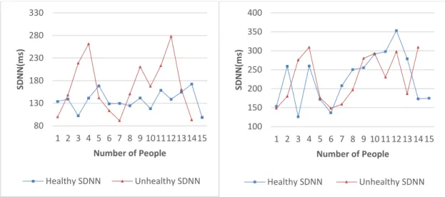
Parameter Response to Exercise

Heart Rate (High responsive)

Stroke Volume (Moderate responsive) Pulse Pressure (Increased Stroke Volume)

(Moderate responsive) Cardiac Output (High responsive)

Table 1. Cardiovascular Responses to Exercise

2.3 Stroke Volume Variability (SVV)

Pulse pressure is the difference between systolic pressure and diastolic pressure. Pulse pressure can be used as an indicator of stroke volume because of the relationships between pressure, volume, and compliance [10]. Compliance of a blood vessel is the volume the vessel can hold at a given pressure. Therefore, if arterial compliance is constant, arterial

(25)

14

pressure depends on the volume of blood the artery contains at any moment in time [10]. Stroke Volume Variability is measured by pulse pressure variation over a period.

2.3.1 Stroke Volume

This is the volume of blood ejected by the ventricle on each beat.

2.3.2 Cardiac Output

The total volume of blood ejected from left ventricle per unit time is the cardiac output. Thus, cardiac output depends on the blood volume ejected in a single beat (stroke volume) and the number of beats per minute (heart rate). Cardiac output is approximately 5000 mL/min in a 70-kg man (based on a stroke volume of 70 mL and a heart rate of 72 beats/min) [10].

(26)

15

CHAPTER III

REVIEW OF LITERATURE

3.1 Related Work

Risk of cardiovascular events can be measured using Heart Rate Variability HRV). Data collected may include undetected beats for example. Such data (unclean data) can seriously affect time and frequency analysis of HRV. Data cleaning is therefore an important task in Heart Rate Variability analysis.

A previous study used chi-squared statistics and a correlation-based feature selection method to filter out irrelevant and redundant features [7]. [15] studied preprocessing data by trend removal and removing ectopic beats. They obtained the standard deviation of RR interval time series (SDRR) of 15 healthy patients and 15 patients suffering from congestive heart failure. The analysis shows that the SDRR values of congestive heart failure patients are depressed compared to the healthy group. A summary of methods from nonlinear dynamics (NLD) have shown new insights into heart rate (HR) variability changes under various physiological and pathological conditions as reported in [16].

(27)

16

Detrended Fluctuation Analysis (DFA) [13], a widely-used technique for detecting correlations in time series, is used to discriminate healthy and unhealthy people. Detrended Fluctuation Analysis (DFA) is a method for scaling the long-term autocorrelation of non-stationary signals. It quantifies the complexity of signals using the fractal property. DFA was first proposed by Peng et al. in 1995 [12]. This method is a modified root mean square method for the random walk. Mean square distance of the signal from the local trend line is analyzed as a function of scale parameter. There is a power-law dependence and scaling component is the exponent [13].

Machine learning algorithms can be implemented on HRV and SVV for analysis and prediction of patients’ heart health. Many classification algorithms exist. Caruana et. al. [18] made a landmark study where they did an empirical comparison of ten well-known supervised learning algorithms. Previous studies [18] [19] [20] showed that random forest gives the better result and therefore we chose random forests in our study.

(28)

17

CHAPTER IV

PROBLEM STATEMENT

4.1 Problem Specification

There are many factors which can cause a heart attack like eating habits, smoking, person’s life style, high cholesterol etc. This is the why we should monitor and measure the health of a heart.

The primary goal of our study is to analyze and predict a cardiac event based on the incoming heart signals of firefighters. One such way is to measure the state of a heart is analysis of Heart rate variability (HRV) and Stroke volume variability (SVV).

4.2 Proposed Solution

Our approach is divided into three sub parts.

First, we show that using machine learning algorithms, cardiovascular events can be predicted. Second, we want to validate our approach is sensitive. To validate the sensitivity of our approach we show that the proposed approach is able to identify differences between lying and sitting postures. Having confirmed the sensitivity of our approach, lastly, we

(29)

18

analyze and predict healthy and unhealthy patient’s data with Heart Rate Variability (HRV) and Stroke Volume Variability (SVV) analysis.

Part 1 – Prediction of cardiovascular events using Heart Rate Variability (HRV) of healthy and unhealthy patients.

Part 2 – Heart Rate Variability (HRV) and Stroke Volume Variability (SVV) analysis of patients according to their posture.

Part 3 – Prediction of cardiovascular events using Heart Rate Variability (HRV) and Stroke Volume Variability (SVV) of healthy and unhealthy patients.

4.2.1 Part 1- Prediction of cardiovascular events using HRV of healthy and unhealthy patients

4.2.1.1 Input Data

4.2.1.1.1 Smart Health for Assessing the Risk of Events via ECG Database [22]

This database includes nominal 24-h electrocardiographic (ECG) Holter recordings of 139 hypertensive patients The ECG Holter was performed after a one-month anti-hypertensive therapy wash-out. The patients aged 55 and over (including 49 females and 90 males, age 72 - 7 years), were followed up for 12 months after the recordings to record major cardiovascular and cerebrovascular events.

4.2.1.1.2 Normal Sinus Rhythm RR Interval Database [23]

This database includes beat annotation files for 54 long-term ECG recordings of subjects in normal sinus rhythm (30 men, aged 28.5 to 76, and 24 women, aged 58 to 73).

(30)

19

4.2.1.2 Methodology

There are many packages and tools available for data analysis of RR interval and HRV analysis. In this study, we used the RHRV package in the R environment for data analysis because it is an open source software package for performing HRV analysis. RHRV uses scripting commands which allows analysis of large volumes of records [21]. RHRV extracts ECG (or Electrocardiogram) signals and creates a data structure that contains RR intervals, non-interpolated heart rate and time.

The automatic removal of outliers is performed with the FilterNIHR function [21]. This function implements an algorithm that uses adaptive thresholds for rejecting or accepting beats. The rule for beat acceptation or rejection is to compare the present beat with the previous one, the following one and with an updated mean of the RR Interval. Time series analysis of filtered/non-filtered data is done to capture Standard Deviation (SD) and Mean of RR intervals. Detrended Fluctuation Analysis is done on filtered/non-filtered data to calculate the scaling component. The scaling component distinguishes long or short fluctuations.

In this work, random forest is performed using SD – Standard Deviation, Mean and DFA – Detrended Fluctuation Analysis scaling component to predict cardiovascular events.

4.2.1.3 Results and Analysis

(31)

20

V Occurrence of Cardiovascular Event (YES/NO)

MeanRR Mean of RR Interval

SD Standard Deviation

SDNN Standard Deviation of RR Interval SDRR Standard Deviation of RR Interval

DFA DFA Scaling Component

ntree Number of Trees

mtry Number of variables randomly sampled as candidates at each split

MeanDecreaseGini This is a measure of how each variable contributes to the equality of the nodes and leaves in the resulting random forest. Each time a variable is used to split a node, the Gini coefficient for the child nodes are calculated and compared to that of the original node. The higher the value the more important the variable.

Sensitivity This is the ability of test to correctly identify those patients? who are diseased (true positive rate)

Specificity This is the ability of a test to correctly identify those patients? who are healthy (true negative rate)

Table 2. Terminologies

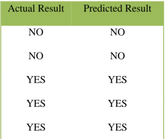
We have used the statistical programming language R to analyze the data. The results are shown below. SDNN represents standard deviation of RR intervals.

(32)

21

Figure 5 (a). SDNN with Data Filtering Figure 5(b). SDNN_without Data Filtering

Figure 6(a). MeanRR with Data Filtering Figure 6(b). MeanRR without Data Filtering

4.2.1.3.1 Prediction Analysis Results with Data Filtering The R code with data filtering is shown below:

randomForest(formula = V ~ Mean + SDNN + DFA, data = data1, ntree = 500, mtry = 3) Type of random forest: classification

80 130 180 230 280 330 1 2 3 4 5 6 7 8 9 101112131415 SD N N (ms) Number of People Healthy SDNN Unhealthy SDNN 100 150 200 250 300 350 400 1 2 3 4 5 6 7 8 9 10 11 12 13 14 15 SD N N (ms) Number of People Healthy SDNN Unhealthy SDNN 400 600 800 1000 1200 1400 1 2 3 4 5 6 7 8 9 101112131415 M e an R R (ms) Number of People

Healthy MeanRR Unhealthy MeanRR

400 600 800 1000 1200 1400 1 2 3 4 5 6 7 8 9 10 11 12 13 14 15 M e an R R (ms ) Number of People

(33)

22

ntree = Number of trees: 500, mtry = No. of variables tried at each split: 3, OOB estimate of error rate: 8.33%

Confusion matrix: MeanDecreaseGini:

NO YES class.error Mean 0.3362796

NO 12 1 0.07692308 SDNN 0.8129905

YES 1 10 0.09090909 DFA 10.2438966

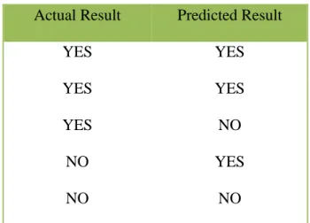
Table 3 below shows actual and predicted result for cardiovascular events with data filtering. This results in High Sensitivity High Specificity.

Actual Result Predicted Result

NO NO

YES YES

Table 3. Actual and Predicted result for Cardiovascular Events with Data Filtering

4.2.1.3.2 Prediction Analysis Results without Data Filtering The R code with data filtering is shown below:

randomForest(formula = V ~ Mean + SDNN + DFA, data = data1, ntree = 500, mtry = 3) Type of random forest: classification

(34)

23

Ntree = Number of trees: 500, mtry = No. of variables tried at each split: 3, OOB estimate of error rate: 29.17%

Confusion matrix: MeanDecreaseGini:

NO YES class.error Mean 6.739465

NO 8 4 0.3333333 SDNN 2.562064

YES 3 9 0.2500000 DFA 2.169304

Below Table 4 shows actual and predicted result for cardiovascular events without data filtering. This results in High Sensitivity Low Specificity.

Actual Result Predicted Result

YES YES

YES NO

NO YES

NO NO

(35)

24

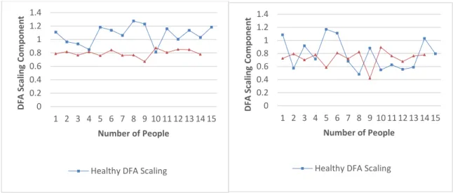
Figure 7(a). DFA Scaling Component Figure 7(b). DFA Scaling Component

With Data Filtering without Data Filtering

Figures 5 and 6 shows that the mean and standard deviation of RR intervals (SDNN and MeanRR) do not yield satisfactory prediction of cardiovascular events, irrespective of whether the data is filtered/cleaned or not. Figure 7(a) shows that using DFA the scaling component is depressed in the records of unhealthy patients compared to healthy patients by 30%.

Table 5 below shows a t-test analysis of the data comparing healthy and unhealthy persons.

0 0.2 0.4 0.6 0.8 1 1.2 1.4 1 2 3 4 5 6 7 8 9 10 11 12 13 14 15 D FA S cal in g C o mp o n e n t Number of People

Healthy DFA Scaling

0 0.2 0.4 0.6 0.8 1 1.2 1.4 1 2 3 4 5 6 7 8 9 10 11 12 13 14 15 D FA S cal in g C o mp o n e n t Number of People

(36)

25

Table 5. t-test Results

These results show that DFA with filtering provides a very reliable classification and can therefore be used as a predictor. The huge impact of filtering is very evident. SDNN with filtering is better than DFA without filtering. The MeanDecreaseGini confirms the t-test results. It shows the importance of the DFA with filtering.

4.2.1.4 Conclusion

In this study, time series analysis is performed for 15 healthy and 14 unhealthy patients’ records aged between 28 and 84. HRV Time series components i.e. RR Interval Mean, Standard deviation and Non-Linear Dynamics measure Detrended Fluctuation scaling component has been calculated.

In this study, we used automatic outlier method for data filtering in the R environment [21]. We get the most accurate results in prediction using Random Forest model with data filtering. Our study shows that DFA Scaling component is depressed in patients who had

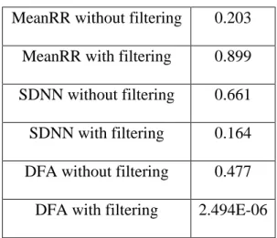
MeanRR without filtering 0.203 MeanRR with filtering 0.899 SDNN without filtering 0.661 SDNN with filtering 0.164 DFA without filtering 0.477

(37)

26

a cardiovascular event in the past. Also, prediction of cardiovascular events is more accurate with data filtering in comparison to non-filtered data.

This study shows that data filtering on the random forest model produces the best sensitivity and specificity.

4.2.2 Part 2 - Heart Rate Variability (HRV) and Stroke Volume Variability (SVV) analysis of patient’s according to their posture

4.2.2.1.1 The EUROBAVAR data set [28]

The database consists of recordings of healthy 23 lying and sitting patients. The recording includes three ECG leads, arterial pressure waveforms.

There are many packages and tools available for data analysis of HRV and SVV analysis. In our study we have used MATLAB to extract features like RR interval, Systolic Pressure and Diastolic Pressure from the dataset. The dataset consists of BP and ECG signals stored in .txt format.

4.2.2.2.1 ABP Beat Detection

The segmentation of the arterial blood pressure (ABP) waveform into individual beats is by a beat detection process. Beat detection is required in extracting arterial blood pressure

(38)

27

features such as systolic pressure, diastolic pressure. We have used an algorithm designed by Zong et al. [29] that detects the onset of each beat in the ABP signal.

The algorithm consists of three components. Low-pass filter, Slope Sum function, Decision rule. The algorithm converts ABP waveform into slope sun function (SSF) to detect the onset of arterial pressure pulses. The slope sum function increases the upslope of the ABP pulse and suppress the remainder of the pressure [29]. The marked onsets allow ABP feature extraction at beat level resolution.

Figure 8. Slope sum function [30]

More information about the algorithm can be found in [29] and its implementation in [30]. [r] = wabp1(abpsignal);

wabp1 function takes ABP signal as an input and outputs onset sample time.

4.2.2.2.2 ABP Feature Selection

There are many ways to extract features from ABP signal. We have used MATLAB WFDB package to extract abpfeatures [30]. abpfeature (wabp, onsettime) function extracts features from ABP waveform such as diastolic pressure, systolic pressure, pulse pressure, mean arterial pressure, pressure area during systole (2 methods), mean of negative slopes (for noise detection), duration of each beat, duration of systole (2 methods), duration of diastole

(39)

28

Heart Rate Variability (HRV) looks at the variation between each heartbeat called RR intervals. RR intervals is measured by calculating the variation between heartbeats within a specific timeframe. Pulse pressure is the difference between systolic pressure and diastolic pressure. Stroke Volume Variability (SVV) is measured by pulse pressure variation over a period. That is why, we have used diastolic pressure, systolic pressure, pulse pressure and duration of each beat to study HRV and SVV analysis.

4.2.2.2.3 Feature Statistics Calculation

Mean and Standard Deviation is calculated for selected ABP features for sitting and lying patients. Statcalculation.m outputs the matrix which consists of the mean and standard deviation of selected ABP features of 23 lying and 23 sitting patients.

The results are shown below. SD represents standard deviation of RR interval, systolic and diastolic pressure.

Figure 9 (a). MeanRR of Lying and Figure 9 (b). SDRR of Lying and Sitting

Sitting Patients Patients

0 0.2 0.4 0.6 0.8 1 1.2 1.4 1 3 5 7 9 11 13 15 17 19 21 RR Mean Number of People Lying Sitting 0 0.1 0.2 0.3 0.4 0.5 0.6 1 3 5 7 9 11 13 15 17 19 21 RR SD Number of People Lying Sitting

(40)

29

Figure 10 (a). Mean Systolic Pressure of Figure 10 (b). SD Systolic Pressure of Lying and Sitting Patients Lying and Sitting Patients

Figure 11(a). Mean Diastolic Pressure of Figure 11(b). SD Diastolic Pressure of Lying and Sitting Patients Lying and Sitting Patients

From these graphs we can conclude that Figure 9(a) shows that RR intervals is depressed in the records of sitting patients compared to lying patients by approximately 11%. Figure

0 20 40 60 80 100 120 140 160 180 1 3 5 7 9 11 13 15 17 19 21 Sy sto lic Pres su re Me an (m m H g) Number of People Lying Sitting 0 2 4 6 8 10 12 14 16 1 3 5 7 9 11 13 15 17 19 21 Sy sto lic Pres su re SD Number of People Lying Sitting 0 20 40 60 80 100 1 3 5 7 9 11 13 15 17 19 21 Dias to lic Pres su re Me an (m m H g) Number of People Lying Sitting 0 1 2 3 4 5 6 1 3 5 7 9 11 13 15 17 19 21 Dias to lic Pres su re SD Number of People Lying Sitting

(41)

30

11(a) shows that the diastolic pressure is higher in the records of sitting patients compared to lying patients by approximately 12% which is significant.

4.2.2.3.1 Prediction Analysis Results with HRV and SVV analysis The R code with HRV and SVV analysis is shown below:

Call:

randomForest(formula = Position ~ SM + DM + SS + DS + PM + RM + RS, data = trainingData, ntree = 500, importance = TRUE)

Type of random forest: classification Number of trees: 500

No. of variables tried at each split: 2 OOB estimate of error rate: 50% Confusion matrix:

Lying Sitting class.error Lying 5 9 0.6428571 Sitting 6 10 0.3750000

Figure 12 below shows the variable importance plot of mean systolic pressure (SM), mean diastolic pressure (DM), mean pulse pressure (PM), mean RR interval (RM), standard deviation systolic pressure (SS), standard deviation of diastolic pressure (DS), standard deviation of RR interval (RS). Figure 12 shows that mean diastolic pressure and mean systolic pressure plays an important role in predicting differences between postures.

(42)

31

Figure 12. VarImpPlot for posture analysis

Table 6 below shows actual and predicted result for lying and sitting patients. This results in Medium Sensitivity Medium Specificity. Table 6 shows that random forest algorithm is able predict 6 lying and 4 sitting patients correctly and 4 patients were incorrectly predicted out of 14 patients.

Lying Sitting

Lying 6 2 Sitting 2 4

Table 6. Actual and Predicted result for lying and sitting Patients with HRV and SVV analysis

(43)

32

Min Max Accuracy MAPE (Mean absolute percentage error)

0.8571 0.25

Table 7. Min Max Accuracy and MAPE for posture analysis

4.2.2.4 Conclusion

In this study, time series analysis is performed for 22 lying and 22 sitting patients’ records HRV and SVV Time series components i.e. Mean, Standard deviation of RR Interval Systolic Pressure, Diastolic Pressure, Pulse Pressure. Figures 9-11 shows that the mean and standard deviation of systolic pressure, diastolic pressure, pulse pressure and RR interval of lying and sitting patients. Figure 11(a) shows that the diastolic pressure is higher in the records of sitting patients compared to lying patients by approximately 12% which is significant. RR intervals is depressed in the records of sitting patients compared to lying patients by approximately 11%. This study shows that both HRV and SVV analysis predictor variables on the random forest model produces the medium sensitivity and specificity.

As a first step in determining the posture of people, we analyzed the lying and sitting patients to determine if a distinction could be made using machine learning techniques between postures using HRV and SVV analysis.

4.2.3 Part 3 -Prediction of cardiovascular events using HRV and SVV of healthy and unhealthy patients

(44)

33

To achieve high accuracy along with HRV analysis we consider SVV and determine a suitable approach that will use HRV and SVV to predict a cardiovascular event with the best sensitivity and specificity.

4.2.3.1.1 The MGH/MF Waveform Database [27]

The database consists of recordings from 250 patients and represents a broad spectrum of physiologic and pathophysiologic states. Individual recordings vary in length from 12 to 86 minutes, and in most cases, are about an hour long. The recording includes three ECG leads, arterial pressure, pulmonary arterial pressure, central venous pressure, respiratory impedance, and airway CO2 waveforms.

4.2.3.1.2 The EUROBAVAR data set [28]

The database consists of recordings of healthy 23 lying and sitting patients. The recording includes three ECG leads, arterial pressure waveforms.

4.2.3.2.1 ECG and ABP Signal Extraction [26]

There are many ways to extract ABP (Arterial Blood Pressure) and ECG signal. In this study, we have used WFDB toolbox available in MATLAB for signal extraction [26]. The WFDB Toolbox for MATLAB is a collection of functions for reading, writing, and processing physiologic signals and time series [26]. rdsamp function is used to extract ECG and ABP (Arterial Blood Pressure) signals. The rdsamp function reads the signal files of

(45)

34

WFDB records by passing recordName, signaList, N, N0, rawUnits, highResolution parameters and returns signal,Fs,tm.

Required Parameters:

• recordName= String specifying the name of the record in the WFDB path or in the current directory.

Optional Parameters are:

• signalList = A Mx1 array of integers. Read only the signals (columns) named in the signalList (default: read all signals).

• N = A 1x1 integer specifying the sample number at which to stop reading the record file (default read all the samples = N).

• N0 = A 1x1 integer specifying the sample number at which to start reading the record file (default 1 = first sample).

• rawUnits = A 1x1 integer (default: 0). Returns tm and signal as vectors according to the following values:

▪ rawUnits=0 - Uses Java Native Interface to directly fetch data, returning signal in physical units with double precision.

▪ rawUnits=1 -returns tm (millisecond precision only!) and signal in physical units with 64 bit (double) floating point precision

▪ rawUnits=2 -returns tm (millisecond precision only!) and signal in physical units with 32 bit (single) floating point precision

▪ rawUnits=3 -returns both tm and signal as 16-bit integers (short). Use Fs to convert tm to seconds.

(46)

35

▪ rawUnits=4 -returns both tm and signal as 64-bit integers (long). Use Fs to convert tm to seconds.

• highResolution = A 1x1 boolean (default =0). If true, reads the record in high resolution mode. Ignored if rawUnits == 0.

• Signal=NxM matrix (doubles) of M signals with each signal being N samples long. Signal data type will be either in double int16 format depending on the flag passed to the function (according to the boolean flags below).

• Fs (Optional) = 1xM Double, sampling frequency in Hz of all the signals in the record.

• tm (Optional) = Nx1 vector of doubles representing the sampling intervals Depending on input flags (see below), this vector can either be a vector of integers (sampling number), or a vector of elapsed time in seconds (with up to millisecond precision only).

4.2.3.2.2 Extract RR intervals for HRV analysis [26]

ann2rr function from WFDB toolbox is used to extract a list of intervals from an annotation file. function takes recordName, annotator, N, N0, consecutiveOnly parameters and returns RR, tms.

Required Parameters:

• record Name = String specifying the name of the record in the WFDB path or in the current directory.

(47)

36

• annotator = String specifying the name of the annotation file in the WFDB path or in the current directory.

Optional Parameters:

• N= A 1x1 integer specifying the sample number at which to stop reading the record file (default read all = N).

• N0 = A 1x1 integer specifying the sample number at which to start reading the annotion file (default 1 = begining of the record).

• consecutiveOnly = A 1x1 boolean. If true, prints intervals between consecutive valid annotaions only (default =true).

• RR = Nx1 vector of integers representing the duration of the RR interval in samples. • tms = Nx1 vector of integers representing the begining of the RR interval in

samples.

4.2.3.2.3 ABP Beat Detection

The segmentation of the arterial blood pressure waveform into individual beats is by beat detection process. Beat detection process is required in extracting ABP features. We have used an algorithm designed by Zong et al. [29] that detects the onset of each beat in the ABP signal.

The algorithm consists of three components. Low-pass filter, Slope Sum function, Decision rule. The algorithm converts ABP waveform into slope sun function (SSF) to detect the onset of arterial pressure pulses. The slope sum function increases the upslope of the ABP pulse and suppress the remainder of the pressure [29]. The marked onsets allow ABP feature extraction at beat level resolution.

(48)

37

Figure 13. Slope sum function [30]

[r] = wabp1(abpsignal);

wabp1 function takes ABP signal as an input and outputs onset sample time.

4.2.3.2.4 ABP Feature Selection

There are many ways to extract features from ABP signal. We have used MATLAB WFDB package to extract abpfeatures [30]. abpfeature (wabp, onsettime) function extracts features from ABP waveform such as diastolic pressure, systolic pressure, pulse pressure, mean arterial pressure, pressure area during systole (2 methods), mean of negative slopes (for noise detection), duration of each beat, duration of systole (2 methods), duration of diastole We only have used diastolic pressure, systolic pressure, pulse pressure and duration of each beat for further data analysis.

4.2.3.2.5 Feature Statistics Calculation

Mean and Standard Deviation is calculated for selected ABP features for 250 unhealthy and 23 healthy patients. Statcalculation_unhealthy.m outputs the matrix which consists of

(49)

38

mean and standard deviation of selected ABP features of 250 ICU patients and Statcalculation_healthy.m outputs the matrix which consists of mean and standard deviation of selected ABP features of 23 healthy lying patients.

4.2.3.2.6 Patients Classification

250 patients from MGH/MF [27] dataset is classified into the following groups • Peripheral Vascular Disease

• Coronary Artery Disease • Carotid Endarterectomy • Cholecystectomy • Endocarditis • Hypertension • Valve Replacement

45 patients who are classified as Peripheral Vascular Disease and Coronary Artery Disease are labeled as unhealthy and 23 healthy lying patients from The EUROBAVAR data set [28] is labeled as healthy and are considered for classifying healthy and unhealthy patients.

4.2.3.2.7 Prediction Model

Random forest is used to classify healthy and unhealthy patients. In our study, a machine learning model is created using random forest and features like mean of diastolic pressure, systolic pressure, pulse pressure, RR interval and standard deviation of diastolic pressure,

(50)

39

systolic pressure, pulse pressure, RR interval is used to predict healthy and unhealthy patients.

Figure 14(a). Mean Systolic Pressure of Figure 14(b). Mean Diastolic Pressure of Healthy and Unhealthy Patients Healthy and Unhealthy Patients

Figure 15(a). Standard Deviation of Systolic Figure 15(b).Standard Deviation of Diastolic Pressure of Healthy and Unhealthy Patients Pressure of Healthy and Unhealthy Patients

0.00 50.00 100.00 150.00 200.00 250.00 1 4 7 101316192225283134374043 Sy sto lic Pres su re Me an (m m H g) Number of People Systolicmean(mmHg)-Unhealthy Systolicmean(mmHg)-Healthy 0.00 20.00 40.00 60.00 80.00 100.00 120.00 1 4 7 101316192225283134374043 Dias to lic Pres su re Me an (m m H g) Number of People Diastolic mean(mmHg)-Unealthy Diastolic mean(mmHg)-Healthy 0.00 10.00 20.00 30.00 40.00 50.00 60.00 1 4 7 101316192225283134374043 Sy sto lic Pres su re SD Number of People Systolic std-Unhealthy Systolic std-Healthy 0.00 5.00 10.00 15.00 20.00 25.00 30.00 1 4 7 101316192225283134374043 Di as to lic Pre ss u re SD Number of People Diastolicstd-Unhealthy Diastolicstd-Healthy

(51)

40

Figure 16. Mean Pulse Pressure of Healthy Figure 17(a). RRMean of Healthy and

and Unhealthy Patients Unhealthy Patients

Figure 17 (b). Standard Deviation of RR of Figure 18. Standard Deviation of Pulse Healthy and Unhealthy Patients Pressure of Healthy and Unhealthy Patients

Figures 14(a) – 18 shows that the mean and standard deviation of systolic pressure, diastolic pressure, pulse pressure and RR interval of healthy and unhealthy patients. Figures 15(a), 15(b) shows that the diastolic pressure, systolic pressure deviation is

0.00 50.00 100.00 150.00 200.00 1 4 7 101316192225283134374043 Pu ls e Pres su re Me an (m m H G ) Number of People Pulsepressuremean(mmHg)-Unhealthy Pulsepressuremean(mmHg)-Healthy 0.00 0.20 0.40 0.60 0.80 1.00 1.20 1.40 1.60 1 4 7 10 13 16 19 22 25 28 31 34 37 40 43 RR Mean Number of People RRmean(sec)-Unhealthy RRmean(sec)-Healthy 0.00 0.10 0.20 0.30 0.40 0.50 0.60 0.70 1 4 7 101316192225283134374043 RR SD Number of People RRstd-Unhealthy RRstd-Healthy 0.00 10.00 20.00 30.00 40.00 50.00 60.00 1 4 7 101316192225283134374043 Pu ls e Pres su re SD Number of People

Pulse Pressure std-Unhealthy Pulse Pressure std-Healthy

(52)

41

depressed in the records of healthy patients compared to healthy patients is around 73% and 53% respectively. This is a very significant difference. Pulse pressure mean, and systolic pressure is depressed in the records of healthy patients compared to healthy patients by approximately 14% and 13% respectively. RR intervals standard deviation is depressed in the records of unhealthy patients compared to healthy patients.

4.2.3.3.1 Prediction Analysis Results with HRV analysis only The R code with HRV analysis only is shown below:

Formula – Call:

randomForest(formula = Healthy ~ RM + RS, data = trainingData, ntree = 500, importance = TRUE)

No. of variables tried at each split: 1 OOB estimate of error rate: 15.62% Confusion matrix:

No Yes class.error No 11 3 0.2142857

Yes 2 16 0.1111111

Figure 19 below shows the variable importance plot of mean RR interval (RM) and standard deviation RR interval (RS). Figure 19 below shows that RR standard deviation plays an important role in predicting healthy and unhealthy people.

(53)

42

Figure 19. VarImpPlot for healthy and unhealthy patients with HRV analysis

Table 8 below shows the actual and predicted result for healthy and unhealthy patients. Table 8 shows that random forest algorithm is able predict 11 healthy and unhealthy patients correctly and 3 patients incorrectly out of fourteen patients. This results in High Sensitivity Low Specificity.

No Yes

No 6 3

Yes 0 5

Table 8. Actual and Predicted result for Healthy and Unhealthy Patients with HRV analysis

(54)

43

0.8928571 0.2142857

Table 9. Min Max Accuracy and MAPE for healthy and unhealthy patients with HRV analysis

4.2.3.3.2 Prediction Analysis Results with HRV and SVV analysis The R code with HRV and SVV analysis is shown below:

Formula – Call:

randomForest(formula = Healthy ~ ., data = trainingData, ntree = 500, importance = TRUE)

No Yes class.error No 11 3 0.2142857 Yes 0 16 0.0000000

Figure 20 below shows the variable importance plot of mean systolic pressure (SM), mean diastolic pressure (DM), mean pulse pressure (PM), mean RR interval (RM), standard

(55)

44

deviation of systolic pressure (SS), standard deviation of diastolic pressure (DS), standard deviation of RR interval (RS). Figure 20 shows that standard deviation of diastolic pressure, standard deviation of RR interval play an important role in predicting healthy and unhealthy people.

Figure 20. VarImpPlot for healthy and unhealthy patients with HRV and SVV analysis

Table 10 below shows the actual and predicted results for healthy and unhealthy patients. Table 10 shows that random forest algorithm is able predict 13 healthy and unhealthy patients correctly and 1 patient incorrectly out of 14 patients. This results in High Sensitivity High Specificity.

(56)

45

No Yes

No 8 1

Yes 0 5

Table 10. Actual and Predicted result for Healthy and Unhealthy Patients with HRV and SVV analysis

0.964 0.071

Table 11. Min Max Accuracy and MAPE for healthy and unhealthy patients with HRV and SVV analysis

4.2.3.3.3 Prediction Analysis Results with SVV analysis The R code with SVV analysis is shown below:

Formula – Call:

randomForest(formula = Healthy ~ SM + DS + DM + SS + PM, data = trainingData, ntree = 500, importance = TRUE)

(57)

46

Figure 21 below shows the variable importance plot of mean systolic pressure (SM), mean diastolic pressure (DM), mean pulse pressure (PM), standard deviation of systolic pressure (SS), standard deviation of diastolic pressure (DS). Standard deviation of diastolic pressure (DS) plays an important role in predicting healthy and unhealthy people.

Figure 21. VarImpPlot for healthy and unhealthy patients with SVV analysis

Table 12 below shows actual and predicted result for healthy and unhealthy patients. Table 12 shows that random forest algorithm is able predict 14 healthy and unhealthy patients correctly out of all 14 patients. This results in High Sensitivity High Specificity.

(58)

47

No Yes No 9 0 Yes 0 5

1 0

Table 13. Min Max Accuracy and MAPE for healthy and unhealthy patients with SVV analysis

4.2.3.3.4 Prediction Analysis Results with SVV analysis with Pulse Pressure Standard Deviation as a predictor variable

Call:

randomForest(formula = Healthy ~ SM + DS + DM + SS + PM + PS, data = trainingData, ntree = 500, importance = TRUE)

No. of variables tried at each split: 2 OOB estimate of error rate: 6.25%

(59)

48

Confusion matrix:

Figure 22 below shows the variable importance plot of mean systolic pressure (SM), mean diastolic pressure (DM), mean pulse pressure (PM), standard deviation of systolic pressure (SS), standard deviation of diastolic pressure (DS), standard deviation of pulse pressure (PS). Figure 22 shows that diastolic pressure and pulse pressure standard deviation plays an important role in predicting healthy and unhealthy people.

Figure 22. VarImpPlot for healthy and unhealthy patients with Standard Deviation of Pulse Pressure and SVV analysis

Table 14 below shows the actual and predicted result for healthy and unhealthy patients. Table 14 shows that random forest algorithm is able predict 14 healthy and unhealthy patients correctly out of 14 patients. This results in High Sensitivity High Specificity.

(60)

49

No Yes No 9 0 Yes 0 5

1 0

4.2.3.3.5 Prediction Analysis Results with Combination of HRV and SVV

To cover maximum number of combinations, out of 7 features i.e. Mean of RR, Systolic Pressure, Diastolic Pressure, Pulse Pressure, Standard Deviation of RR, Systolic Pressure and Diastolic Pressure, a combination of three features are selected to predict the health of person that gives us 35 combinations in total. Figure 23 shows that 5 combinations, namely, Systolic mean + Diastolic Mean + Diastolic Standard Deviation, Systolic Mean + Systolic Standard Deviation + Diastolic Standard Deviation, Systolic Mean + Systolic Standard Deviation + Pulse Pressure Mean, Systolic Mean + Diastolic Standard Deviation + Pulse

(61)

50

Pressure Mean and Systolic Mean + Diastolic Standard Deviation + RR Mean produces high accuracy.

Figure 23. Min-Max Accuracy and MAPE for Combination of HRV and SVV analysis

Figure 24 below shows the deviation of RR, systolic pressure, diastolic pressure and pulse pressure of healthy and unhealthy people. Standard deviation of pulse pressure, diastolic pressure and systolic pressure is higher in unhealthy patients than healthy people.

0.00 0.10 0.20 0.30 0.40 0.50 0.60 0.70 0.80 0.90 1.00 SM +DM + SS SM +DM + P M SM +DM + R S SM +S S+ PM SM +S S+ R S SM +DS +R M SM +PM+ R M SM +R M+ R S DM + SS +PM DM + SS +R S DM + DS + R M DM + P M+ R M DM + R M+ R S SS +DS +R M SS +PM+ R M SS +R M+ R S D S+ PM+ RS PM+ R M+ R S MIn -Ma x Acc u ra cy /MAP E Predictor Variables

(62)

51

Figure 24. Variability Plot of Healthy and Unhealthy People

4.2.3.3.6 Prediction of Gender with HRV and SVV analysis

114 patients who are classified as having Peripheral Vascular Disease, Coronary Artery Disease, Carotid Endarterectomy, Cholecystectomy, Endocarditis, Hypertension, Valve

0.00 10.00 20.00 30.00 40.00 50.00 60.00 1 3 5 7 9 11 13 15 17 19 21 23 25 27 29 31 33 35 37 39 41 43 Sta n d ar d De viat ion Number of People

Systolic std-Unhealthy Diastolicstd-Unhealthy

RRstd-Unhealthy Systolic std-Healthy

Diastolicstd-Healthy RRstd-Healthy

(63)

52

Replacement are labeled as unhealthy. These are considered for predicting the persons gender with HRV and SVV statistics. Random forest algorithm is used as a classifier. Call:

randomForest(formula = Sex ~ ., data = trainingData, ntree = 500, importance = TRUE) Type of random forest: classification

Number of trees: 500

Female Male class.error Female 36 3 0.07692308 Male 16 1 0.94117647

Figure 25 below shows the variable importance plot of mean systolic pressure (SM), mean diastolic pressure (DM), mean pulse pressure (PM), mean RR interval (RM), standard deviation of systolic pressure (SS), standard deviation of diastolic pressure (DS), standard deviation of RR interval (RS). Figure 25 shows that diastolic pressure standard deviation plays an important role in predicting healthy and unhealthy people.

(64)

53

Figure 25. VarImpPlot for gender analysis

Table 16 shows actual and predicted result of a gender. Table 16 below shows that random forest algorithm is able predict nineteen male and female patients correctly and five out twenty-four of patients incorrectly. This results in Medium Sensitivity High Specificity.

Female Male

Female 18 0

Male 5 1

(65)

54

0.896 0.1041667

4.2.3.3.7 Prediction of Age with HRV and SVV analysis

114 patients who are classified as having Peripheral Vascular Disease, Coronary Artery Disease, Carotid Endarterectomy, Cholecystectomy, Endocarditis, Hypertension, Valve Replacement are labeled as unhealthy. A Sample of 100 patients above age 50 is selected from unhealthy dataset and grouped into old and very old. A patient with age between 50-70 is labeled as old and a patient with age between 50-70-88 is labeled as very old. The patient’s age is predicted using HRV and SVV statistics. Random forest algorithm is used as a classifier.

Call:

randomForest(formula = Age ~ ., data = trainingData, ntree = 500, importance = TRUE) Type of random forest: classification

Number of trees: 500

No. of variables tried at each split: 2 OOB estimate of error rate: 35.48%