Temporal Uncertain Databases
Jiaqi Ge1, Yuni Xia1, and Jian Wang2 1
Department of Computer & Information Science, Indiana University Purdue University Indianapolis, Indiana, USA, 46202
2
School of Electronic Science and Engineering, Nanjing University, Jiangsu, China, 210023
1
{jiaqige,yxia}@cs.iupui.edu,[email protected]
Abstract. Uncertain sequence databases are widely used to model data with inaccurate or imprecise timestamps in many real world applica-tions. In this paper, we use uniform distributions to model uncertain timestamps and adopt possible world semantics to interpret temporal uncertain database. We design an incremental approach to manage tem-poral uncertainty efficiently, which is integrated into the classic pattern-growth SPM algorithm to mine uncertain sequential patterns. Extensive experiments prove that our algorithm performs well in both efficiency and scalability.
Keywords: Temporal Uncertainty, Sequential Pattern Mining
1
Introduction
Sequential pattern mining (SPM) provides inter-transactional analysis for times-tamped data and mines frequent patterns in sequence databases. However, it is very common that timestamps of events might be inaccurate or imprecise in real applications. And temporal uncertainty is usually caused by the following reasons:
– The exact time of an event is often unavailable. For example, in temperature monitoring sensor networks, temperatures are measured periodically. The exact time of a sudden temperature change is unknown, and it can only be inferred from raw data probabilistically.
– Temporal uncertainty arises when data are collected in different temporal scales. For example, a handhold GPS device may update the position every 10 minutes; while a GPS on a fast-moving vehicle may report every 5 sec-onds. And the temporal relationship is uncertain between two events within different granularities.
– Temporal uncertainty can also be caused by aggregation operations on tem-poral scales. For example, an economic indicator may be aggregated from weekly or monthly data to represent high level abstracted information in this time period.
__________________________________________________________________________________________
This is the author's manuscript of the article published in final edited form as:
Ge, J., Xia, Y., & Wang, J. (2015). Towards Efficient Sequential Pattern Mining in Temporal Uncertain
Databases. In Advances in Knowledge Discovery and Data Mining (pp. 268-279). Springer International
Publishing. http://dx.doi.org/10.1007/978-3-319-18032-8_21
– Temporal uncertainty is also used to protect privacy and confidentiality. Precise time information in monitoring data usually is not released if there is a potential to identify individuals. Therefore, uncertainty is introduced to original time points, which is unquantifiable and unknown by the data user. A time seriesT ={t,(t+ 1), . . . ,(t+n)} that bounds a set of consecutive timestamps is used to model an uncertain event time in probabilistic temporal databases, where it assumes that all events are defined within the same discrete time domain. However, this model becomes inaccurate and inconvenient when data are actually collected in different time scales. Instead, we use uniform dis-tributions to represent uncertain timestamps in our model, which do no rely on any discrete time domain.
It is very important to carefully manage temporal uncertainty in SPM prob-lems; otherwise, the mined patterns might be inaccurate. Possible world seman-tics is widely used to interpret probabilistic databases; however, it also brings efficiency and scalability challenges to uncertain SPM problems. Therefore, in this paper, we propose an efficient SPM algorithm in temporal uncertain se-quence databases. Our main contributions are listed as follows:
(1) We model uncertain timestamps by uniform distributions. And we use pos-sible world semantics to interpret this type of temporal uncertainty.
(2) We develop a novel approach to manage temporal uncertainty in the process of mining uncertain sequential patterns by a pattern-growth algorithm.
(3) We conduct extensive experiments to demonstrate the efficiency and scala-bility of our algorithm.
2
Related Works
Data mining in uncertain databases has been an active area of research recently. A lot of traditional database and data mining techniques have been extended to be applied to uncertain data [1]. Particularly, Muzammal and Raman pro-posal the SPM algorithm in probabilistic database using the expected support as the measurement of pattern frequentness [10]; however, expected support has inherent weakness in mining high-quality sequential patterns[12]. Zhao et al. measure pattern frequentness using possible world semantics and propose a pattern-growth uncertain SPM algorithm [14, 15]. Miliaraki et al use approxi-mation with probabilistic guarantee to improve the efficiency of uncertain SPM problem [9]. A dynamic programming approach is used to mine probabilistic spatial-temporal frequent sequential patterns [8]. However, these methods are all designed for sequence databases with accurate timestamps.
Dyreson and Snodgrass introduced probabilistic temporal databases which models uncertain timestamp by a set of time points with equal probabilities [4]. Zhang et al. proposed a pattern recognition algorithm in temporal uncertain streams[13]; while pattern queries in temporal uncertain sequences is studied in [16]. However, our work distinguishes from the above in that we use uniform distributions to represent uncertain timestamps, which is more flexible in mod-eling data collected from different scales. Meanwhile, the above works focused on
sid eid T I 1 1 [100,103] {A,C} 1 2 [102,105] B 2 1 [160,163] A 2 2 [162,164] B 2 3 [163,166] B 2 4 [167,168] C
Fig. 1.An example of uncertain database
sid eid t I 1 1 102.5 {A,C} 1 2 103.9 B 2 1 163 A 2 2 162 B 2 3 165 B 2 4 166 C
Fig. 2.An example of a possible world
matching patterns in one sequence, while the SPM problem is more complicated because it mines patterns from a large number of uncertain sequences so that their techniques cannot be directly employed.
3
Problem statement
3.1 Temporal Uncertain Sequence Database
A temporal uncertain sequence database contains a collection of uncertain se-quences, and an uncertain sequence is a set of temporal uncertain events. A temporal uncertain event is represented by e= hsid, eid, T, Ii. Here sid is the sequence-id,eidis the event-id andhsid, eidiidentifies a unique event. Note that events are not guaranteed to be ordered by theireids. An uncertain timestamp T is modeled by a uniform distributionT ∼U(t−, t+), where [t−, t+] is the range ofT.I is an itemset that describes the content of evente.
Fig. 1 shows an example of temporal uncertain database. A sequence is a list of events that are associated with the samesidand an event identified bysid=i and eid = j is denoted by eij. For example, e11 = h1,1,{[100,103]},{A, C}i indicates that event{A, C}occurs at timeT, whereT ∼U(100,103) is uniformly distributed within 100 and 103.
3.2 Temporal Possible Worlds
We use possible world semantics to interpret temporal uncertain databases. Tem-poral possible worlds of an uncertain databaseDare generated by instantiating all possible values of each uncertain timestamp. Fig. 2 shows an example a tem-poral possible worlds that are instantiated from the uncertain database in Fig. 1, in which the time point of an event is randomly drawn from the corresponding uncertain timestamps.
It is widely assumed that uncertain sequences inDare mutually independent, which is known as thetuple-level independence [7, 1] in probabilistic databases. Meanwhile, event time are also assumed to be independent of each other [3, 5,
6, 14], which can be justified by the fact that events are often observed indepen-dently in real applications. Thus, the probability density function (pdf) of the possible words can be computed by Equation (1).
f(w) = m Y i=1 f(di) = m Y i=1 ni Y j=1 f(Tij =tij) (1)
Wheredi is a sequence in the databaseD andeij is an event indi.m=|D|
is the number of sequences inD andni=|di|is the number of events indi. Let
Tij ∼U(t−ij, t
+
ij) be the uncertain time of event eij, then its pdf f(Tij =tij) is
shown in Equation (2). f(Tij=tij) = ( 1 t+ij−t−ij , t∈[t − ij, t + ij] 0 ,otherwise (2)
3.3 Uncertain Sequential Pattern Mining Problem
A sequential patternα=hX1· · ·Xniissupported by a sequenceβ =hY1· · ·Ymi,
denoted by α β, if and only if there exists integers {k1, . . . , kn} so that we
have Xi.I⊆Yki.I (∀i∈[1, n]) andl≤Yki+1.t−Yki.t≤h(∀i∈[1, n−1]). Here
l =mingapis the minimal time gap constraint between two adjacent events of αandh=maxgapis the maximal time gap constraint.
In deterministic databases, a sequential patternsis frequent if and only if it satisfiessup(s)≥ts, wheresup(s) is the total number of sequences that support
sandtsis the user-defined minimal threshold. However, In an uncertain database
D, the frequentness of s is probabilistic and it can be computed by Equation (3).
P(sup(s)≥ts) =
Z
sup(s|w)≥ts
f(w)dw (3)
Wherewis a possible world in whichsis frequent andf(w) is the pdf ofw. The SPM problem in temporal uncertain databases can be defined as follows.
Given a minimal support ts, a minimal frequentness probability threshold tp, a
minimal time gap l and a maximal time gap h, find every probabilistic frequent
sequential pattern s in a temporal uncertain database, which has P(sup(s) ≥
ts)≥tp.
4
Solution
4.1 Frequentness Probability
SupposeD={d1, . . . , dn}is a temporal uncertain database andsis a sequential
pattern. Because d1, . . . , dn in D are mutually independent, the probabilistic
sup(s) =
n
X
i=1
sup(s|di) (4)
Wheresup(s|di) (∀i ∈[1, n]) is a Bernoulli random variable, whose success
probability is P(sup(s|di) = 1) =P(sdi).
sup(s) is a Poisson-Binomial random variable, since it is the sum ofn inde-pendent but non-identical Bernoulli random variables. And the probability mass function (pmf) ofsup(s) isP(sup(s) =i) =pi, wherepi is the probability that
the support ofs in D equals toi (i∈[1,|D|]). Here we adopt the Fast Fourier Transform (FFT) technology in [14] to compute the pmf ofsup(s) in O(nlogn) time . Thereafter, thefrequentness probability ofsis computed by Equation (5).
P(sup(s)≥ts) = X i≥ts pi= 1− X i<ts pi (5)
Where,ts is the minimal support threshold andpi =P(sup(s) =i) (i∈[1, n])
is the probability that the support of s in D equals to i. Given the minimal frequentness probability threshold tp, sis probabilistically frequent if and only
ifP(sup(s)≥ts)≥tp.
4.2 Support Probability
We first define the minimal possible occurrence of a sequential pattern s in an uncertain sequence d.
Definition 1. Given a sequential patternsand an uncertain sequenced, a
sub-set d0 of d(e.g. d0 ⊆d) is called a minimal possible occurrence ofs if and only
if (1) P(sd0)>0; (2) ∀d00⊂d0, P(sd00) = 0.
For example, in Fig. 1,{e21, e22}and{e21, e23}are two minimal possible oc-currences of the sequential patternhA,Biin the sequences2; while{e21, e22, e23} is not a minimal occurrence of hA,Bi. Then the support probability P(s d) can be computed by Equation (6), since event timestamps are independent.
P(sd) =
N
X
i=1
P(sosi) (6)
Here osi (i = 1, . . . , N) are N minimal possible occurrences of s, and the
computation ofP(sosi) is discussed in section 4.3.
4.3 Probability of satisfying time constraints
Let os={ek1, . . . , ekn} be a minimal possible occurrence of sequential pattern
s=hs1, . . . , sni. SupposeTi is the uncertain time of the eventeki, thenP(s
constraints l ≤ Ti+1 −Ti ≤ h, ∀i ∈ [1, n). Here l is the minimal time gap
between two adjacent timestamps andhis the maximal time gap.
A naive approach of computingP(hT1· · ·Tni) is to use thechain rule, which
is shown in Equation (7). P(hT1· · ·Tni) = Z · · · Z l≤ti−ti−1≤h f(Tk1 =t1, . . . , Tkn=tn)dt1· · ·dtn = Z · · · Z l≤ti−ti−1≤h f(tn|t1· · ·tn−1)· · ·f(t2|t1)f(t1)dt1· · ·dtn (7)
However, this method is usually too complex in practice. Therefore, we design a new approach to compute P(hT1· · ·Tni) efficiently.
Basic case. We first consider the basic case of two uncertain timestampsX∼ U(x−, x+) andY ∼U(y−, y+). Given time constraints mingap=l,maxgap= h,P(hXYi) can be computed in Equation (8).
P(hXYi) = Z min(y+,x++h) max(y−,x−+l) Z min(x+,y−l) max(x−,y−h) 1 (x+−x−)(y+−y−)dxdy (8)
Equation (8) is decomposed into p deterministic cases, if [y−, y+] is divided intopdisjoint subintervals by the endpoints{x++l, x−+l, x++h, x−+h} as
[y−, y+] =S[y− i , y + i ],∀i∈[1, p]. HereYk ∼U[yk−, y + k] is a uniformly distributed
random variable, andP(hXYi) can be computed by Equation (9). P(hXYi) = p X k=1 P(hXYki)P(Y =Yk) (9) Where P(Y = Yk) = (y+k −y − k)/(y
+−y−). We use a geographic method to
computeP(hXYki) in O(1) time, which is shown in Equation (10).
P(hXYki) = Sk Ak = (1/2)∗(L1+L2)∗H (yk+−yl k)(x+−x−) (10) Where,Ak is the area of the rectangle defined by the 2-dimensional uniform
distribution ofX and Yk, andSk is the area withinAk which satisfies the time
constraints. HereH =y+k −y−k,L1andL2are computed as follows. L1=max(0, L01), L01=min(y−k −l, x + )−max(yk−−h, x−) L2=max(0, L02), L 0 2=min(y + k −l, x +)−max(y+ k −h, x −)
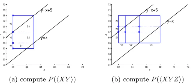
Fig. 3(a) shows an example of computing P(hXYi) with l = 0 and h= 5, where X ∼ U[60,63] and Y ∼U[62,68]. There two endpoints {63,65} within the range ofY, which divide [62,68] into three disjoint subintervals as [62,68] = [62,63]∪[63,65]∪[65,68].
60 62 64 66 68 70 59 60 61 62 63 64 65 66 67 68 69 70 X Y y=x y=x+5 S3 S2 S1 Y3 Y2 Y1 (a) computeP(hXYi) 62 64 66 68 70 72 61 62 63 64 65 66 67 68 69 70 71 72 Y Z Y1 Y2 Y3 y=x y=x+5 Z1 Z2 Z3 (b) computeP(hXY Zi)
Fig. 3.An example of compute the probability of satisfying time constraints
LetY1∼U[62,63],Y2∼U[63,65] andY3∼U[65,68], then we have P(Y =Y1) = 1 6 P(hXY1i) = S1 A1 = 2.5 3 P(hXY1i ∩Y1) = 2.5 18 P(Y =Y2) = 2 6 P(hXY2i) = S2 A2 = 6 6 P(hXY2i ∩Y2) = 1 3 (11) P(Y =Y1) = 3 6 P(hXY3i) = S3 A3 = 4.5 9 P(hXY3i ∩Y3) = 1 4 Thereafter,P(hXYi) =P3 i=1P(hXYii ∩Yi) = 0.72.
General case. Given uniformly distributed uncertain timestamps T1, . . . , Tn,
suppose the range ofTnis divided intopsub-partitions as [t−n, t
+ n] = Sp i=1[t−ni, t + ni], andTni ∼U(t − ni, t +
ni) is a uniform distributed random variable, then we can
com-puteP(hT1· · ·Tni) by Equation (12). P(hT1, . . . , Tni) = p X i=1 P(hT1, . . . , Tnii)∗P(Tn=Tni) = p X i=1 P(hT1, . . . , Tnii ∩Tni) (12)
WhereP(hT1· · ·Tnii) can be computed by Equation (13).
P(hT1, . . . , Tnii) = q X j=1 P( T1, . . . , T(n−1)j )P( T(n−1)jTni )P(T(n−1)j) = q X j=1 P(T(n−1)jTni )P(T1, . . . , T(n−1)j ∩T(n−1)j) (13)
Lets0=hs1, . . . , sn−1ibe a sequential pattern by removing the last element of
s=hs1, . . . , sni. In SPM process, we have already computedP(
T1, . . . , T(n−1)j
T(n−1)j) in searchings
0. Thus, we can save and reuse these values when we search
patterns, in order to avoid repeated computation.
Given another uncertain time Z ∼ U[65,70], Fig. 3(b) shows the process of computing P(hXY Zi) by reusing previous computational results. First, we compute potential end points by the ranges ofY1,Y2 andY3as follows.
z11=y−1 +l= 62, z12=y+1 +l= 63, z13=y−1 +r= 67, z14=y1++h= 68 z21=y−2 +l= 63, z22=y+2 +l= 65, z23=y−2 +r= 68, z24=y2++h= 70 z31=y−3 +l= 65, z32=y+3 +l= 68, z33=y−3 +r= 70, z34=y3++h= 73
Therefore, the range of Z is divided into three disjoint sub-partitions as [65,70] = [65,67]∪[67,68]∪[68,70]. Let Z1 ∼ U[65,67], Z2 ∼ U[67,68] and Z3∼[68,70]. Here we take the computation ofP(hXY Z1i) in Equation (14) as an example. P(hXY Z1i) = 3 X i=1 P(hXYii ∩Yi)P(hYiZ1i) (14)
WhereP(hXYii ∩Yi) is already computed in Equation (11). Referring to
Equa-tion (10), we can compute P(hY1Z1i) = 1, P(hY2Z1i) = 1, P(hY3Z1i) = 1/3. Thereafter, we haveP(hXY Z1i) = 1∗ 1 6∗ 2.5 3 + 1∗ 2 6∗ 6 6+ 1 3∗ 3 6∗ 4.5 9 = 0.5555. Similarly, we can computeP(hXY Z2i) = 0.6111 and P(hXY Z3i) = 0.3333. Therefore, we arrive to the final resultP(hXY Zi) = 0.4∗0.5555 + 0.2∗0.6111 + 0.4∗0.3333 = 0.4777.
4.4 Uncertain SPM Algorithm
We integrate our uncertain management approach into the classic SPM algo-rithm PrefixSPan[11]. There are two major modifications to the original Pre-fixSpan in our uncertain SPM algorithm.
(1) We project the database by minimal possible occurrences. Suppose os =
{ek1, . . . , ekn} is a minimal possible occurrence of sin sequence d. The
projec-tion of d w.r.t. os, denoted by d|os, eliminates any event ei in d if P(ei.T ≥
ekn.T +mingap) = 0. A projected database D|s ={d1|o1,...,op, . . . , dt|o1,...,oq}
is a collection of projected sequences, where di|o1,...,op ={di|o1, . . . , di|op} is a
set ofpprojected sequences ofdi w.r.t. to the minimal occurrenceso1, . . . , op of
s in di. For example, in Fig. 1, if we set mingap = 1 and let s =hABi, then
D|s={d2|o1,o2}, whered2|o1={e23, e24} andd2|o2={e24}.
(2) We save intermediate computational results for each minimal possible occur-rence. Let os ={ek1, . . . , ekn} be a minimal possible occurrence ofs in d and
Ti =eki.T ∀i∈[1, n]. Suppose the range [t
−
n, t+n] ofTn is divided intok
subin-tervals [t−n, t+
n] =
S
[t−ni, t+
ni] (∀i∈[1, k]), then we computepi=P(hT1, . . . , Tnii)
by Equation (12) and save the results in the form as T(os) = {[t−n1, t +
n1] : p1, . . . ,[t−nk, t
+
nk] : pk}. Therefore, we can reuse T(os) in searching longer
se-quences.
We adopt the pattern-growth approach to search new patterns in Algorithm 1. We first mine frequent items inD|s, denoted byI={i1, i2, ..., in}. This process
ALGORITHM 1:USPM(s, D|s)
Input: sequential patterns, uncertain projected databaseD|s,
minsup=ts,minprob=tp
Output:L: a set of frequent sequential patterns Find all frequent itemsI={i1, i2, ..., in}inD|s if D|s=φorI=φthen
returnL
end
foreach itemi∈Ido
s0=s+{i}
fordi|o1,...,on∈D|sdo
fordi|oj ∈di|o1,...,on do
construct a projected sequencedi|os0 fromdi|oj
computeT(os0) fromT(os
j) indiby Equation (12) and Equation (13)
end
compute the support probabilityP(s0di) by Equation (6).
end
use FFT to compute the Poisson Binomial distribution ofsup(s0)
if P(sup(s0)≥ts)≥tpthen L=L∪ {s0};
USPM(D|s0, s0);
end end
is straightforward because it does not need to consider temporal uncertainty. A candidate pattern s0 =s+{i}is generated for each i∈I. Then, we extract all minimal possible occurrences ofs0 and construct their projected databases. For each minimal possible occurrence os0 ofs0, we compute and save its probability
of satisfying time constraints by Equation (12) and Equation (13).
We compute the support probability of s0 in each uncertain sequence by Equation (6). Thereafter, we adopt the FFT technique in [14] to compute the Poisson Binomial distribution of the overall support sup(s0). The frequentness probability is computed in Equation (5), by which we can determine if s0 is a probabilistic frequent sequential pattern. The searching process stops until no frequent patterns are mined.
5
Evaluation
5.1 Synthetic data generation
We use the IBM market-basket data generator [2] to generate synthetic sequence datasets in different scales with the following parameters: (1)C: number of se-quences; (2)T: average number of transactions/itemsets per data-sequence; (3)L: average number of items per transaction/itemset per data-sequence; (4)I: num-ber of different items.
11020 50 100 0 200 400 600 800 1000 C(*1000) running time(s) NV uSPM 5 10 15 20 30 0 200 400 600 800 1000 1200 1400 1600 1800 2000 T running time(s) NV uSPM 2 4 6 8 10 0 500 1000 1500 2000 L running time(s) NV uSPM 5 10 30 50 100 0 50 100 150 200 250 300 350 400 I(*100) running time(s) NV uSPM
Fig. 4.Scalability of uSPM in synthetic uncertain datasets
8 5 3 2 1 0 100 200 300 400 500 600 700 800 minsup(*0.1%) running time(s) NV uSPM 4 5 6 7 8 9 0 20 40 60 80 100 120 minprob(*0.1) running time(s) NV uSPM 5 10 20 40 80 0 100 200 300 400 500 600 maxgap running time(s) NV uSPM
Fig. 5.Effect of parameters in synthetic uncertain datasets
To add temporal uncertainty, we replace a point-value timestamp t in the original synthetic datasets by a uniform distribution in [(1−r)∗t,(1 +r)∗t], where r is randomly drawn from the uniform distribution U(0,1). We name the generated synthetic dataset by parameters. For example, the dataset named T4L10I1C10 indicates thatT = 4,L= 10,I= 1∗1000 andC= 10∗1000.
Our uncertain sequential pattern mining algorithm is calleduSPM for short. Recall from Section 4.3 that a naive method to compute the probability of an occurrence satisfying time constraints is to directly evaluate Equation (7) us-ing chain rule. This naive method is implemented and abbreviate as N V. We compare uSPM with NV to evaluate the performance of our algorithm. All the experiments were done in the desktop with Intel(R) Core (TM) Duo CPU @ 2.33GHz and 4GB memory.
5.2 Scalability and efficiency
In Fig. 4, we compare the running time of uSPM and NV on synthetic datasets with different scales, where we setminsup= 0.5%,minprob= 0.7,mingap= 1, andmaxgap= 10. We initially haveC = 10 000,T = 4,I = 10 000 andL= 2. In Figigure 4(a), C varies from 1 000 to 100 000; In Fig. 4(b), T varies from 5 to 30; In Fig. 4(c),Lvaries from 2 to 10; and In Fig. 4(c) I varies from 500 to 10 000.
In Fig. 4, we observe the following phenomenons: (1) uSPM is significantly faster than NV under every setting of the parameters, which proves the effective-ness of our temporal uncertainty management approach. (2) The running time increases with the increment of C, T,L, as the increment of these parameters
10 8 6 4 2 0 500 1000 1500 2000 minsup(%) running time(s) NV uSPM
(a) running time
10 8 6 4 2 0 100 200 300 400 500 minsup(%) # of Patterns (b) number of patterns
Fig. 6.Performance of uSPM in real stock dataset
generates larger synthetic datasets. (3) The running time drops slightly with the increment ofI, because there are less repeated items in sequences whenI is set to a larger value.
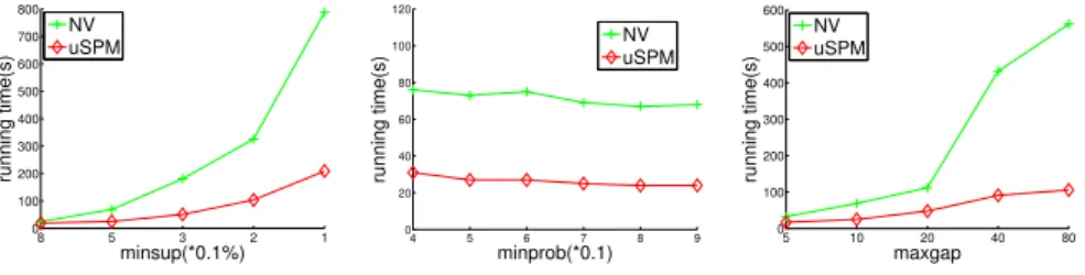
Fig. 5 compares the running time of uSPM and NV with different of user-defined parameters in the dataset T4L2I10C10. We initially setminsup= 0.2%, minprob= 0.7,mingap= 1, andmaxgap= 10. In Fig. 5(a),minsup decreases from 0.8% to 0.1%; in Fig. 5(b), minprob varies from 0.4 to 0.9; andmaxgap varies from 5 to 80 in Fig. 5.
In Fig. 5, we observe that: (1) The running time of uSPM increase with the decrement ofminsup; however, the performance is relatively stable to the varia-tions ofminprob. The probabilistic support of a sequential pattern is bounded to its expected value (Chernoff bound) so that the frequentness of a large number of patterns become deterministic. This explains why the running time of uSPM does not fluctuate significantly in Fig. 5(b). (3) The running time of uSPM in-creases when we set a larger value tomaxgap. This is intuitive because a larger maxgapindicates a less strict constraint of sequential patterns.
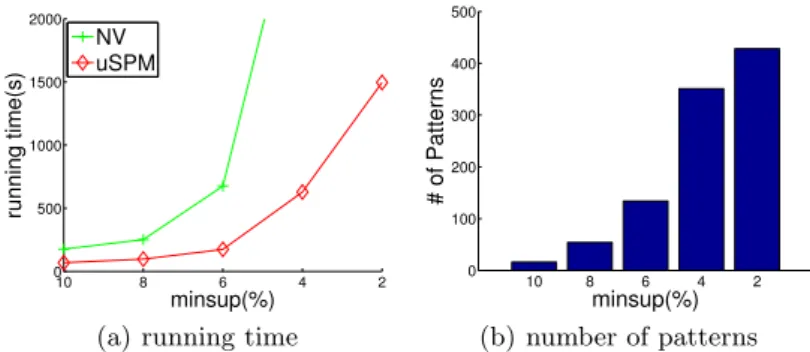
We also apply uSPM to a real world stock market dataset. The prices for 882 stocks are extracted from Shanghai Stock Exchange Center in 16 weeks from 12-03-2012 to 03-24-2013. Each stock corresponds to a sequence. We define three events such as price going up (+), going down (−) and no change (0). An uncertain event is aggregated from consecutive events. For example, if price goes up at time 1, 2 and 3, then we aggregate them to form an uncertain event ([1,3], +).
Here we setminprob= 0.7,mingap = 1 andmaxgap= 5. Fig. 6(a) shows that the running time of uSPM in the stock dataset increases with the decrement ofminsup. As we only define three distinct events, there are many repeated items in sequences; however, uSPM still significantly outperforms NV in this dataset. In Fig. 6(b), we can see that the number of frequent sequential patterns in the stock dataset increases significantly when we decrease the value ofminsupfrom 10% to 2%. And a mined pattern h+,−,+,−i from this dataset reveals that stock prices are fluctuated in general during the time when data are collected, which is consistent with intuitive observations.
6
Conclusion
In this paper, we study the problem of mining probabilistic frequent sequential patterns in databases with temporal uncertainty. We design an incremental ap-proach to manage temporal uncertainty efficiently and integrate it into classic pattern-growth SPM algorithm. The experimental results prove that our algo-rithm is efficient and scalable.
References
1. C. C. Aggarwal and P. S. Yu. A survey of uncertain data algorithms and applica-tions. IEEE Trans. on Knowl. and Data Eng., 21(5):609–623, May 2009.
2. R. Agrawal and R. Srikant. Fast algorithms for mining association rules in large databases. InVLDB, pages 487–499, 1994.
3. T. Bernecker, H.-P. Kriegel, M. Renz, F. Verhein, and A. Zuefle. Probabilistic frequent itemset mining in uncertain databases. InSIGKDD, pages 119–128, 2009. 4. C.E.Dyreson and R.T.Snodgrass. Supporting valid-time indeterminacy. InTODS,
1998.
5. C. Chui and B. Kao. A decremental approach for mining frequent itemsets from uncertain data. InPAKDD, pages 64–75, 2008.
6. C. Chui, B. Kao, and E. Hung. Mining frequent itemsets from uncertain data. In
PAKDD, pages 47–58, 2007.
7. J. Jestes, G. Cormode, F. Li, and K. Yi. Semantics of ranking queries for probabilis-tic data. IEEE Transactions on Knowledge and Data Engineering, 23(12):1903– 1917, 2011.
8. Y. Li, J. Bailey, L. Kulik, and J. Pei. Mining probabilistic frequent spatio-temporal sequential patterns with gap constraints from uncertain databases. InICDM, pages 448–457, 2013.
9. I. Miliaraki, K. Berberich, R. Gemulla, and S. Zoupanos. Mind the gap: Large-scale frequent sequence mining. InSIGKDD, pages 797–808, 2013.
10. M. Muzammal and R. Raman. Mining sequential patterns from probabilistic databases. InPAKDD, pages 210–221, 2011.
11. J. Pei, J. Han, B. Mortazavi-asl, H. Pinto, Q. Chen, U. Dayal, and M. chun Hsu. Prefixspan: Mining sequential patterns efficiently by prefix-projected pat-tern growth. InICDE, pages 215–224, 2001.
12. Y. Tong, L. Chen, Y. Cheng, and P. S. Yu. Mining frequent itemsets over uncertain databases. In Proceeding of the VLDB Endowment, volume 5, pages 1650–1661, 2012.
13. H. Zhang, Y. Diao, and N. Immerman. Recognizing patterns in streams with imprecise timestamps. Proc. VLDB Endow., 3(1-2):244–255, 2010.
14. Z. Zhao, D. Yan, and W. Ng. Mining probabilistically frequent sequential patterns in uncertain databases. InEDBT, pages 74–85, 2012.
15. Z. Zhao, D. Yan, and W. Ng. Mining probabilistically frequent sequential pat-terns in large uncertain databases. InIEEE Transactions on Knowledge and Data Engineering, volume 26, pages 1171–1184, 2013.
16. Y. Zhou, C. Ma, Q. Guo, L. Shou, and G. Chen. Sequence pattern matching over time-series data with temporal uncertainty. InEDBT, pages 205–216, 2014.