Using the analytic hierarchy process in evaluating decision alternatives

No. 1 2010

Paweł CABAŁA*

USING THE ANALYTIC HIERARCHY PROCESS

IN EVALUATING DECISION ALTERNATIVES

In this paper the method of the Analytic Hierarchy Process (AHP) is described. At the beginning the general assumptions of the method are characterized and discussed. These are related to assump-tions held within General Systems Theory. Then the problems of pairwise comparisons of elements, with its use of a specific scale, as well as the resulting reciprocal matrix are presented. There are many ways of estimating the eigenvectors of this matrix. These eigenvectors reflect weights of pref-erences. Despite the fact that we are able to evaluate the consistency of judgements the problem of acceptable weights still remains. Therefore, by way of an illustration, the method for the sensitivity analysis of preferences is also discussed in the paper.

Keywords: hierarchical structure of a system, pairwise comparisons, reciprocal matrix, preference

analysis, sensitivity analysis

1. General Characteristics of the Method

Management problems are complex, which means that they are often described and defined in too general a way. Reduction of this complexity requires not only specialist knowledge, but also analytical skills supported by the right methodology. One concept which assists in the analysis of the complexity of management problems is the Ana-lytic Hierarchy Process (AHP).

The AHP is one of the suggestions for solutions concerning the construction and application of multi-criteria evaluation systems. It originated in the 1970s in the United States. Over the past three decades, it has been the subject of much methodo-logical research and has also been used with success in the solution of many practical problems.

* Department of Management Process, Cracow University of Econimics, Rakowicka 27, 31-510 Kraków, e-mail: cabalap@uek.krakow.pl

The originator of the AHP is Thomas Saaty, who, as a professor at Wharton Busi-ness School in Philadelphia in the early 70s, worked out the methodological founda-tions of the concept. Wider interest in the method came about in the 80s after the pub-lication of The Analytic Hierarchy Process by the renowned publishers MCGRAW-Hill

[13]. It seems that the method grew from the foundation of considerations on general systems theory as it is a development of the attempts to provide a formal description of one of the basic features of a system, which L. BERTALANFFY called the “hierarchical

order” [2].

The AHP can be defined as a process of hierarchizing a system in order to carry out a wide-ranging evaluation and final selection of one of the alternative solutions to a particular problem. The method can also be understood more broadly as a theory of measurement using quantitative and/or qualitative data.

The work involved in solving a problem using the AHP comprises two phases. In the first phase, the hierarchical structure of the system is prepared. In brief, this means identifying the elements of the system and grouping these elements according to a hierarchy. All the elements located on a higher hierarchical level act on the ele-ments situated a level lower. This activity is similar to the construction of a goal tree. In the second phase, individual elements are evaluated and the consistency of the evaluation is checked. The evaluation works by comparing all pairs of elements at a given level from the point of view of each element located a level higher in the pre-viously constructed hierarchical structure. The result of the comparisons is a set of matrices which, after normalisation and examination of consistency, form the basis for the final evaluation of the system.

2. Identifying the structure of a hierarchical system

Systematic thinking assumes the existence of a hierarchy. One of the originators of general systems theory – Ludwig von Bertalanffy – wrote: “We currently ‘see’ the Universe as a vast hierarchy, from elementary particles, atomic nuclei, molecules, and multimolecular compounds, up to the wealth of structures between molecules and cells (…). A similar hierarchy is to be found in both ‘structures’ and ‘functions’. Ulti-mately, the structure (and so the order of parts) and the function (the order of proc-esses) may be exactly the same thing” [2, p. 57].

Every system is a set of elements which are mutually related. These elements form a particular hierarchy, which is crucial for the existence and survival of many systems, both natural and human-made. A system is a multi-layer arrangement. The levels are differentiated by internal structure and functions. The functions of elements on a lower level are subordinated to the functions of elements on a higher level. The proper func-tioning of the higher levels depends on the proper funcfunc-tioning of the lower levels.

In the broadest terms, we can isolate two types of hierarchy: structural and func-tional [12, p. 30–31]. A structural hierarchy indicates the relationships between the component parts of complex systems, where these relationships are understood as an arrangement in terms of structural properties (e.g. shape, volume, colour, age). Struc-tural hierarchy mirrors the way in which the human mind analyses complexity by dis-tinguishing kinds, classes, groups, sub-groups, types, sets, and subsets. Functional hierarchy, on the other hand, appears in the relationships between elements on a given hierarchical level. Elements on a given level are thus not completely equivalent. Functional hierarchy means that there are also relationships between them of the type: “less important”, “more important”.

The above division of hierarchies may seem controversial. If a functional hierarchy exists, after all, then in essence it is a form of structural hierarchy. Hierarchical rela-tionships as a rule mean that there is a relationship of subordination and superiority, but functional relationships refer to horizontal co-ordination. On the other hand, in isolating hierarchical levels we are indicating a subordination which need not neces-sarily be subordination to the same degree.

Overall Welfare of the Nation

National

Economy Health, SafetyEnvironment PoliticalFactors Cheap Electricity

Unavoidable Pollution

Natural Resources Independence

Centralization Political cooperat-iveness Accidents & Long-term Risks Foreign Trade Capital Resources No Big

Power Plants Power PlantCoal-fired power plantNuclear Focus:

Criteria:

Sub-criteria:

Alternatives:

Fig. 1. An example hierarchical structure concerning Finland’s energy policy

Source: [11]

In the creation of hierarchical structures which are meant to reflect specific practical problems it needs to be remembered that human perception is limited. This is also why it is suggested that the number of elements at a given hierarchical level, as well as the number of hierarchical levels themselves, for a given research problem should not ex-ceed nine. In the AHP, as will be shown later, the scale of evaluations used also has a similar range. This suggestion is a consequence of experimental psychological re-search, which shows that people (e.g. chess players) can deal with information

describ-ing just a few facts simultaneously. One of the first experiments of this type was carried out in the 1950s by George Miller, who showed that we can generally deal with seven facts at once, plus or minus two [9]. A greater number of facts causes an individual to lose the thread, which means that they are unable to make a reliable evaluation.

Figure 1 shows an example of a hierarchical structure for a decision problem which was solved using AHP (in reality it is an extract from a more elaborate structure which was used in practice). Specific hierarchical levels are given numbers or are de-scribed in words. In this example, as in many others, the goal is at the highest level, whereas the second level comprises the selection criteria. The base of the hierarchy comprises the alternatives.

As well as presenting a given system in the form of a hierarchical structure, it is no less important to show the relative influence of individual elements of that structure on the functioning of the whole. In the second phase of the AHP, pairwise comparisons of all elements are carried out, as well as an evaluation of the consistency of these com-parisons.

3. Preference Analysis

Preferences in the AHP are determined on the basis of pairwise comparisons, which involves the evaluation of each element with all the other elements at a given hierarchical level. An element is a defined object such as a decision variant or an evaluation criterion. The reference point for the comparisons is an element which is higher in the hierarchy.

n j i a_ij], where , 1,2,..., [ = , (1) j i a_ij =1 for = , (2) j i a a ji ij= for ≠ 1 . (3)

The preference matrix with the above properties is the result of a pairwise com-parison of all the elements at a given hierarchical level with respect to a defined fea-ture (attribute, criterion). Property (1) means that we are dealing with a matrix of di-mensions n×n, where n is the number of elements compared. Property (2) is an expression of the principle of identity, which says that two identical elements com-pared with each other are not differentiated by preference. A lack of difference in preferences is expressed by the number 1. Therefore, all the element values along the diagonal of the matrix are equal to 1.

In comparisons between elements at a given hierarchical level, we assume the principle that an element on line i is always compared with an element in column j. And so aij indicates how much more (or less) important the i-th element is than the

j-th element. In the AHP we also assume that preferences are reciprocal, which is ex-pressed by property (3). If we state that the i-th element is, for instance, x times more important than the j-th element (e.g. aij = x), then we automatically assume that the j-th element is 1/x as important as the i-th element (aji = 1/x).

In pairwise comparison of n elements, it is sufficient for the comparison values to be entered above the diagonal in matrix A. The remaining values equal 1 (the diago-nal) or are the reciprocals of the values above the diagonal. Therefore, the total num-ber of comparisons necessary equals

2 ) 1 (n− n

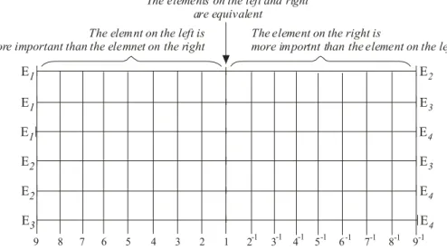
. Furthermore, when experts perform pairwise comparisons they do not need to enter their results in a table like matrix A. Better results can be obtained by preparing suitable scales. For example, for 4 ele-ments which are to be compared pairwise, it suffices to draw up the 6 appropriate combinations in the form shown in figure 2.

E₁ E₂

The elemnt on the left is

more important than the elemnet on the right The element on the right ismore importnt than the element on the left The elements on the left and right

are equivalent E₁ E₃ E₁ E₄ E₂ E₃ E₂ E₄ E₃ E₄ 9 8 7 6 5 4 3 2 1 2 3 4 5 6 7 8 9-1 -1 -1 -1 -1 -1 -1 -1

Fig. 2. An example of pair combinations for the 4 elements being examined

The issue of comparisons concerns the situation when a precise measurement of all the parts of features of the elements to be analysed is not possible. Therefore, a suitable evaluation scale is introduced which will allow the analyst to estimate the preferences between the sets of combined elements. In the AHP, it is assumed that the scale is from 1 to 9, where element i is equal to or more important than element j, and that the scale is the reciprocal of that scale (1/2, 1/3, …1/9) when element i is less important than element j. During the comparisons, it is suggested that odd numbers

from 1 to 9 are used. If there are doubts in setting the preferences, use even numbers. A detailed interpretation of the evaluation scale is given in table 1.

Table. 1. Evaluation scale used in pairwise comparisons

Intensity of

importance Definition Explanation

1 Equal importance Two activities contribute equally to the objective 3 Moderate importance Experience and judgement slightly favour activity

over another

5 Strong Importance Experience and judgement strongly favour activity_{over another} 7 Very strong importance An activity is favoured very strongly over another;_{its dominance demonstrated in practice} 9 Extreme importance The evidence favouring one activity over another is_{of the highest possible order of affirmation}

2,4,6,8 For compromise between the_{above values}

Sometimes one needs to interpolate a compromise judgement numerically because there is no good word to describe it

Reciprocals of above

If activity i has one of the above nonzero numbers assigned to it when compared with activity j, then j has the reciprocal value when compared with i

A comparison mandated by choosing the smaller element as the unit to estimate the lager one as a multiple of that unit

Rationals Ratios arising from the scale If consistency were to be forced by obtaining_{numerical values to span the matrix} n 1.1–1.9 For tied activities When elements are close and nearly indistinguish-_{able; moderate is 1.3 and extreme is 1.9}

Source: [12, p. 73].

In practical situations we have to combine elements which are expressed by differ-ent features. These comparisons are only possible when they are performed in relation to a specific reference point. As has already been mentioned, this reference point is an object higher in the hierarchical structure of the research problem. Using the scale above, a reciprocal matrix [aij] is created where aij is the expert’s evaluation express-ing the preference of the i-th element in relation to the j-th.

The eigenvector w matching the maximum eigenvalue λmax of the pairwise com-parison matrix A is the final expression of the preferences between the investigated elements. The problem of determining the eigenvector leads to the solution of matrix A’s characteristic equation. The characteristic function is as follows1_:

1 _{As is widely known, the issue of the method of finding eigenvalues and eigenvectors for matrices}

has been examined by many distinguished mathematicians, such as Lagrange, Le Verrier, Jacobi and Laplace. Some of these have been discussed in Kowalczyk’s work [7, pp. 233–284].

λ λ λ λ λ − − − = − = nn n n n n n a a a a a a a a a a I A f 1 1 1 2 22 21 1 12 11 ... ... ... ... ... ... | | ) ( (4)

and its respective characteristic equation f(λ) = |A – λI| = 0 is presented in the form of

the polynomial 1 ... ₁ 0

1

0 n+c n− + +cn− +cn=

c λ λ λ .

The eigenvectors of matrix A are each column and non-zero vector Xi, for which the following equality occurs:

0 )

(A−λ_i X_i= . (5)

If we assume that Xi = w for λmax, eigenvector we are interested in is the solution to the following equation:

w

Aw=λ_max . (6)

Below three methods of finding the eigenvector corresponding to λmax are given:

Saaty’s method, the power method, and the geometric mean method.

Saaty’s Method. This can be defined as a method of normalised arithmetic aver-ages. The prepared pairwise comparison matrix is normalised. As a result of the nor-malisation, matrix A is transformed into matrix B = [bij]. The elements of matrix B are calculated according to the following formula:

∑

Calculating the preference between the elements under investigation (eigenvector w = [wi]) is performed by calculating the arithmetic averages from the row of the nor-malised comparison matrix. The components of this vector are calculated according to the formula: n b w n j ij i

∑

The maximum eigenvector is calculated according to the equation:

∑

The above method for calculating the eigenvector and eigenvalue gives good re-sults when there is high consistency in the pairwise comparisons. The result obtained

is an approximation, but is more precise the more consistent the evaluations are. The indubitable virtue of this method is that the calculations are less laborious than under the other two methods.

The power method allows the calculation of a preference eigenvector value with any degree of precision. In successive iterations we approximate the eigenvector which, meeting the required level of precision ε, will be the final preference vector. The iterations (steps) are denoted by the letter k, where k = 1, 2, ..., m. Therefore, the total number of iterations equals m. Each step successively obtains a better approxi-mation wk _{to this eigenvector of matrix A. If in a given step the precision level ε is met} (i.e. k equals m), the final approximation of the eigenvector is the preference vector (wm_{). The first approximation to the eigenvector equals:}

T 1 1 1 1_=[n− _,...,n− _,...,n− _] w . (10)

For successive approximations (k≥ 2) an auxiliary value dk _{= Aw}k–1 _{is introduced.}

Successive approximations to the desired vector are equal to:

T 1,..., ,..., ] [ k n k i k k _{= w w w} w , (11)

∑

The end of the calculation is reached when

) | | (max 1 ,... 1 − <ε − = k i k i n i

Λ

At each step we calculate the approximate maximum eigenvalues according to the following formula:

∑

The geometric mean method. This is an alternative to the abovementioned meth-ods. The equation for simple calculation of the approximate component values of the eigenvector using the geometric averaging method looks as follows:

n ij n j n i n ij n j i a a w ₁ 1 1 1 ) ( ) ( Π Σ Π = = = _{. (15)}

Independent of the calculation method, the components of the eigenvector w are understood as an expression of the preference between the elements under investiga-tion. The sum of these components equals 1, i.e. Σn_{=1 i} =1.

i w

As already mentioned, in the AHP all elements at a given level are compared with each other pairwise. This comparison takes place in relation to each element one level higher in the hierarchical structure. Therefore, the result of the comparisons is a set of matrices and their respective eigenvectors.

We create a matrix C, whose columns are the preference vectors v for the elements located on a given level of the hierarchical structure. Finally, the preference vector x is equal to the product of matrix C and vector w, which is simultaneously the preference vector for the elements one level higher in the hierarchical structure:

Cw

x= . (16)

This is how we derive the solution for the research problem in question.

4. Evaluation of the comparisons’ consistency

The pairwise comparison matrix is consistent (consistency matrix) when the fol-lowing equality is true for each i, j, and k: aikakj = aij. This formula is an expression of the transitivity of preferences, i.e. if for example E2 f E4 (element E2 is more

impor-tant than element E4) and E4 _f E1, then E2 _f E4.

When the elements compared are expressed in the same units of measurement and we use a suitably precise measuring tool, then pairwise comparison is unnecessary. The an-swer to the question of how much more important one element is than the others is given simply by the combination of the measurements of all the elements. It is worth investi-gating the properties of the comparison matrix in the case of precise measurements.

The pairwise comparison matrix for precise measurements of any number of ele-ments is a consistency matrix. The initiator of the AHP, Thomas Saaty, discovered certain properties of this type of matrix which allow the verification of the consistency of the measurements in situations when there is no opportunity for taking precise measurements.

We can list the measurements as w1, w2, ..., wn. If we compare the measurement for element i with the measurement of element j, the result of the comparison is a value expressed as the ratio between wi and wj. The opposite comparison, between j and i, is clearly therefore expressed as the ratio between wj and wi. If we accept this symme-try of comparison, the matrix created has a particularly interesting property which turns out to be useful in examining the degree of consistency when we do not have the requisite measuring tool. We can see that:

⎥ ⎥ ⎥ ⎥ ⎦ ⎤ ⎢ ⎢ ⎢ ⎢ ⎣ ⎡ = ⎥ ⎥ ⎥ ⎥ ⎦ ⎤ ⎢ ⎢ ⎢ ⎢ ⎣ ⎡ ⎥ ⎥ ⎥ ⎥ ⎦ ⎤ ⎢ ⎢ ⎢ ⎢ ⎣ ⎡ n n n n n n n w w w n w w w w w w w w w w w w w w w w w w w w w M M M O M M 2 1 2 1 2 2 1 2 2 2 1 2 1 2 1 1 1 / ... / / / ... / / / ... / / . (17)

If we label the pairwise comparison matrix A, and the vector of the measurements w, we can say:

w

Aw=n . (18)

As we have already discovered, the calculation of the preference vector leads to the solution of the following equation:

w

Aw=λ_max , (19)

where λmax is the matrix’s largest eigenvalue. This is a result of the fact that the com-parison matrix for precise results has the following property:

n = max

λ . (20)

If matrix A is a consistency matrix, as in the above case comprising precise meas-urements, then each row is multiplied by the constant for that row. In this case all the eigenvalues λi(i = 1, 2, ..., n), with the exception of one, are equal to zero. In matrix algebra, the following statement is well-known:

) ( 1 A tr n i i=

∑

where tr(A) is the trace of matrix A (i.e. the sum of all the elements on its diagonal)2. Therefore, in the case of proportional consistency matrices the equality λmax = n is true because all the remaining eigenvalues equal 0.

Based on the above arguments, we can formulate the following statement: matrix A is consistent if and only if λmax = n. As we shall see, this statement plays a

funda-mental role in evaluating the consistency of the comparisons; when we have no precise measurements, i.e. when the comparisons are made by an expert based on his knowl-edge, experience and intuition.

In the case of inconsistent comparison matrices the following statement is true:

n ≥ max

λ . (22)

This statement may be proved by assuming that the result of any comparison be-tween two elements contains a certain degree of error in comparison with a consistent

matrix which shows precise measurements. If we assume that wi and wj are precise measurements, and that the expert’s evaluation equals these measurements, then:

1 = i j ij _w w a , (23) n w w a i j n j ij =

∑

In most estimates, however, the above equalities do not hold. If the deviation from precise measurement is denoted by the coefficient δij, then:

j i ij ij _w w a =(1+δ ) , (24)

where δij > –1. As we know, aij is the expert’s estimate. The condition for proportion-ality for pairwise comparison matrix A, is that aij =

ji

a

1

. Therefore, using the equation Aw = λmaxw, we can say:

0 1 1 2 1 max− =

∑

As can be seen, the number expressed by the difference λmax – n is a measure of the deviation of the inconsistent matrix from the consistent comparison matrix. On this basis, we can construct indicators showing the consistency of the expert’s estimates. For evaluations of consistency, T. Saaty proposes the following solution:

1 CI max − − = n n λ . (26)

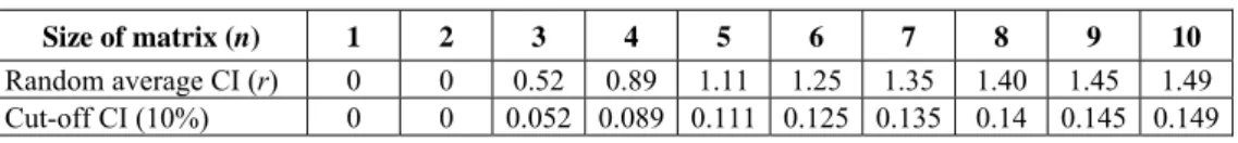
Table 2. Random and cut-off consistency indexes

Size of matrix (n) 1 2 3 4 5 6 7 8 9 10

Random average CI (r) 0 0 0.52 0.89 1.11 1.25 1.35 1.40 1.45 1.49 Cut-off CI (10%) 0 0 0.052 0.089 0.111 0.125 0.135 0.14 0.145 0.149

Source: (SAATY, 2001, p. 83).

The consistency index (CI) refers to the average of the remaining solutions of the characteristic equation for the inconsistent matrix A. This index increases in propor-tion to the inconsistency of the estimates. Using the suggested comparison scale (1/9, 1/8, …1/2, 1,2, 3…9) values for the pairwise comparisons are generated randomly.

Table 2 shows the CI values for matrices with dimensions from 1 to 10. Matrices of a higher degree do not concern us because, following our assumption, the maximum number of compared elements should not exceed nine.

The CI values for random pairwise comparisons (r) should vary considerably from the experts’ estimates3_{. The expression of this difference is the Consistency}

Ratio (CR). % 100 ) 1 ( CI CI CR max − − = = n r n average random λ . (27)

Finally, the experts’ estimates are deemed acceptable if the CR is less than 10%. In the subject literature, other methods of calculating the preference vector than those shown above can be found. Comparative studies of methods based on the maximal eigenvector are contained in the papers: [5], [15]. An interesting algo-rithm for calculating the maximal eigenvector of a proportional matrix in the AHP was proposed by COGGER and YOU [3]. These authors propose that the comparison matrix should comprise of just zeroes below the diagonal. This premise makes the search for the maximal eigenvector considerably easier, but on the other hand may lead to false estimates [5]. There exist other methods of determining the preference vector for pairwise comparison matrices outside of those based on the maximal eigenvector. An alternative method to the AHP for analysing proportional matrices, based on geometrical averages, is presented by CRAWFORD and WILLIAMS [4].

5. Using the AHP in the selection process

for a project variant

A project may be implemented in three different ways, which we will call vari-ants I, II and III. Seven criteria (K1 to K7) have been selected for the evaluation and final choice of the project to be implemented. The starting point for selecting the evaluation criteria is the project goal. The hierarchical structure for the project is shown in figure 3.

3 _{Random average consistency indexes are calculated based on a large number (e.g. 1000) of}

ran-domly generated matrices. The values of r given in the literature may therefore vary to an insignificant degree.

Project Goal

Criterion K2 Criterion K3 Criterion K4 Criterion K5

Criterion K1 Criterion K6 Criterion K7

Variant I Variant II Variant III Fig. 3. The hierarchical structure of the example project

First of all, we have to set the preferences concerning the evaluation criteria. Each of the seven selected criteria will be compared pairwise. The comparisons take place in relation to the project goal (the element immediately higher in the hierar-chy). The results of the comparisons, in the form of a preference matrix, are shown in table 3.

Table 3. Preference matrix for the evaluation criteria for the project variants

Goal K1 K2 K3 K4 K5 K6 K7 K1 1 2 1/5 1/5 2 1/9 3 K2 1/2 1 1/5 1/5 2 1/8 2 K3 5 5 1 1 4 1/5 6 K4 5 5 1 1 3 1/4 5 K5 1/2 1/2 1/4 1/3 1 1/7 1 K6 9 8 5 4 7 1 8 K7 1/3 1/2 1/6 1/5 1 1/8 1

We determine the maximal eigenvector for the criteria using Saaty’s method. To do this we normalise the preference matrix (table 4).

Table 4. Normalised comparison matrix for the project evaluation criteria

K1 K2 K3 K4 K5 K6 K7 wi K1 0.047 0.091 0.026 0.029 0.100 0.057 0.115 0.0664 K2 0.023 0.045 0.026 0.029 0.100 0.064 0.077 0.0520 K3 0.234 0.227 0.128 0.144 0.200 0.102 0.231 0.1810 K4 0.234 0.227 0.128 0.144 0.150 0.128 0.192 0.1720 K5 0.023 0.023 0.032 0.048 0.050 0.073 0.038 0.0411 K6 0.422 0.364 0.640 0.577 0.350 0.512 0.308 0.4531 K7 0.016 0.023 0.021 0.029 0.050 0.064 0.038 0.0344

The preference vector w determined represents the order of the criteria (final col-umn of table 4). The values calculated therefore allow us to organise the evaluation criteria for our project variants in the following order:

K7 K5 K2 K1 K4 K3 K6_{f f f f f f} .

Next, we check the consistency of the comparisons. We calculate the maximal ei-genvalue: 4671 . 7 ) ( 1 1 max=

∑

From the random consistency index table (table 2) we see that for a 7-dimen-sional matrix, the coefficient r is 1.35. Based on this we can calculate the consis-tency ratio: % 77 . 5 % 100 ) 1 7 ( 35 . 1 7 4671 . 7 % 100 ) 1 ( CI max ₌ − − = − − = n r n λ .

It follows from the calculations that the pairwise comparisons for the evaluation of the project alternatives are consistent, because the CR for the comparison matrix is less than 10%.

The next step in the AHP is to evaluate the specific project variants with respect to the criteria presented. For each criterion separately, we evaluate all the alternatives. The calculations (Saaty method) are shown in table 5.

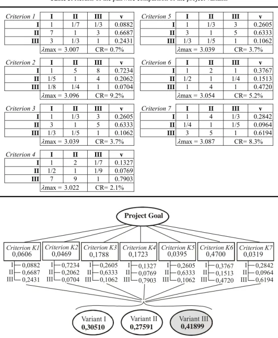
The calculations shown in tab. 5 enable us to create matrix C, whose columns are the eigenvectors of the pairwise comparisons of the project variants with respect to all the evaluation criteria placed above them in the hierarchy. Matrix C is then multiplied by the preference vector w for the evaluation criteria. In this way we obtain the final preference vector x for the project variants under consideration. In the calculations we have used the preference vector for the evaluation criteria obtained using the power method. ⎥ ⎥ ⎥ ⎦ ⎤ ⎢ ⎢ ⎢ ⎣ ⎡ = ⎥ ⎥ ⎥ ⎥ ⎥ ⎥ ⎥ ⎥ ⎥ ⎦ ⎤ ⎢ ⎢ ⎢ ⎢ ⎢ ⎢ ⎢ ⎢ ⎢ ⎣ ⎡ ⎥ ⎥ ⎥ ⎦ ⎤ ⎢ ⎢ ⎢ ⎣ ⎡ = = 41899 . 0 27591 . 0 30510 . 0 0319 . 0 4700 . 0 0395 . 0 1723 . 0 1788 . 0 0469 . 0 0606 . 0 6194 . 0 4720 . 0 1062 . 0 7903 . 0 1062 . 0 0704 . 0 2431 . 0 0964 . 0 1513 . 0 6333 . 0 0769 . 0 6333 . 0 2062 . 0 6687 . 0 2842 . 0 3767 . 0 2605 . 0 1327 . 0 2605 . 0 7234 . 0 0882 , 0 Cw x .

Table 5. Results of the pairwise comparison of the project variants

Criterion 1 I II III v Criterion 5 I II III v

I 1 1/7 1/3 0.0882 I 1 1/3 3 0.2605

II 7 1 3 0.6687 II 3 1 5 0.6333

III 3 1/3 1 0.2431 III 1/3 1/5 1 0.1062

λmax = 3.007 CR= 0.7% λmax = 3.039 CR= 3.7%

Criterion 2 I II III v Criterion 6 I II III v

I 1 5 8 0.7234 I 1 2 1 0.3767

II 1/5 1 4 0.2062 II 1/2 1 1/4 0.1513

III 1/8 1/4 1 0.0704 III 1 4 1 0.4720

λmax = 3.096 CR= 9.2% λmax = 3.054 CR= 5.2%

Criterion 3 I II III v Criterion 7 I II III v

I 1 1/3 3 0.2605 I 1 4 1/3 0.2842 II 3 1 5 0.6333 II 1/4 1 1/5 0.0964 III 1/3 1/5 1 0.1062 III 3 5 1 0.6194 λmax = 3.039 CR= 3.7% λmax = 3.087 CR= 8.3% Criterion 4 I II III v I 1 2 1/7 0.1327 II 1/2 1 1/9 0.0769 III 7 9 1 0.7903 λmax = 3.022 CR= 2.1% 0,0882 0,6687 0,2431 0,7234 0,2062 0,0704 0,2605 0,6333 0,1062 0,1327 0,0769 0,7903 0,2605 0,6333 0,1062 0,3767 0,1513 0,4720 0,2842 0,0964 0,6194 0,0319 0,0606 0,0469 0,1788 0,1723 0,0395 0,4700 I II III I II III I II III I II III I II III I II III I II III 0,30510 0,27591 0,41899 Project Goal

Criterion K2 Criterion K3 Criterion K4 Criterion K5

Criterion K1 Criterion K6 Criterion K7

Variant I Variant II Variant III

Fig. 4. Selection of the project variant to be implemented

In synthetic form, the results of the evaluation are shown in figure 4.

From the calculations, it can be seen that variant II is the least beneficial. The most beneficial, on the other hand, is variant III.

6. Sensitivity analysis of the evaluation system

Experience with the AHP shows that the final result of the pairwise comparisons is generally consistent with the preferences of experts according to the ordinal scale. Sometimes there are doubts about the result according to the ratio scale, which we obtain in the form of the eigenvector (weight) determined. Hurley has proposed a solution which enables the weights to be changed while maintaining the ranking order which was determined (2001).

We introduce a coefficient α≥ 0, which is the index of the component values of the comparison matrix, i.e. the first matrix A is transformed into the matrix [a_ij∝]. If α > 1, we obtain more dispersed weights, and when α < 1 the weights become more concen-trated. A change in the α coefficient does not, however, change the ranking order.

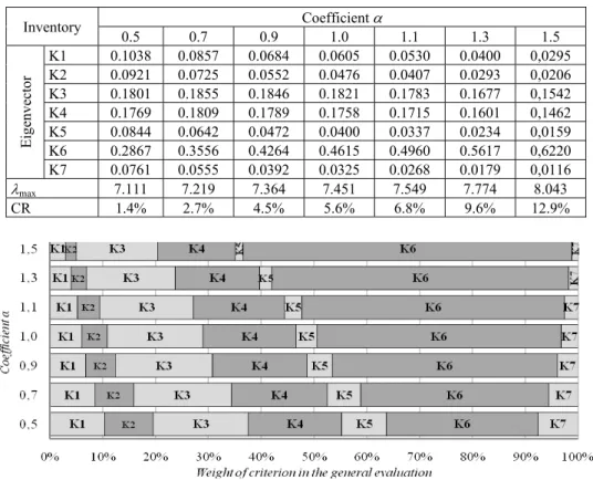
Table 6. Results of the sensitivity analysis for the preference eigenvector for the project evaluation criteria

Coefficient α Inventory 0.5 0.7 0.9 1.0 1.1 1.3 1.5 K1 0.1038 0.0857 0.0684 0.0605 0.0530 0.0400 0,0295 K2 0.0921 0.0725 0.0552 0.0476 0.0407 0.0293 0,0206 K3 0.1801 0.1855 0.1846 0.1821 0.1783 0.1677 0,1542 K4 0.1769 0.1809 0.1789 0.1758 0.1715 0.1601 0,1462 K5 0.0844 0.0642 0.0472 0.0400 0.0337 0.0234 0,0159 K6 0.2867 0.3556 0.4264 0.4615 0.4960 0.5617 0,6220 Eigenvector K7 0.0761 0.0555 0.0392 0.0325 0.0268 0.0179 0,0116 λmax 7.111 7.219 7.364 7.451 7.549 7.774 8.043 CR 1.4% 2.7% 4.5% 5.6% 6.8% 9.6% 12.9%

As can be seen, the α coefficient does not change the ranking order of elements at a given hierarchical level. It may, however, have a crucial influence on the order of elements located lower in the hierarchy.

We will now look at how the results of the sensitivity analysis for the evaluation criteria influence the weights of the project variants. We are therefore establishing the influence of a change in the weights of the evaluation criteria – obtained as a result of the abovementioned sensitivity analysis – on the final preferences with respect to the project variants. The results of this simulation are shown in figure 6.

Fig. 6. The influence of a change in the weights of the evaluation criteria

on the weights of the project variants

As we can easily see, the maintenance of the ranking order for the evaluation crite-ria does not guarantee the maintenance of the ranking order for the project vacrite-riants. In figure 6, it can be seen that for α = 0.5 and α = 0.7 the second variant (W2) is pre-ferred to the first variant (W1). The simulation did not, however, influence a change in the position of the third variant, which has the highest rank for all acceptable values of the coefficient α. It is only when α is lowered to 0.07 that a change in the most pre-ferred variant occurs. For α = 0.7, the preference vector for the project variants has the form x = [0.30230 0.34897 0.34873]T.

7. Conclusion

Assurance of the comprehensiveness and consistency of evaluation plays a con-siderable role in the diagnosis of complex systems. The AHP shown here is one of

the proposals for solutions which order the evaluation process and improve the deci-sion-making process. In applying it, however, it should be remembered that exces-sive algorithmisation may cause a lack of critical thinking in the evaluator. Fre-quently, logically consistent solutions give results which contradict common sense. This is a comment which also applies to many other methods of multi-criteria evaluation.

The direction of further research in this field in the most recent literature on the subject concerns the Analytic Network Process (ANP), which allows for the possibil-ity that elements situated lower in the hierarchy may influence elements located on higher levels [17].

The effectiveness of pairwise comparison methods is dependent on the measure-ment scales used and the guidelines concerning the comparison process. In essence, the result of a preference analysis is a subjective judgement, burdened with error not only because of an unsatisfactory level of consistency, but also insufficient knowledge and experience on the part of the evaluator. In complex management problems it is therefore necessary to call upon the advice of experts, and at the same time investigate the degree of consistency in group preferences.

References

[1] AL-SUBHI AL –HARBI, K.M, Application of the AHP in project management, International Journal of Project Management, 2001, Vol. 19, 19–27.

[2] BERTALANFFY L., Ogólna teoria systemów, PWN, Warszawa 1984.

[3] COGGER K.O., YOU P.L., Eigen weight vectors and least distance approximation for revealed pref-erence in pairwise weight ratios, Journal of Optimization Theory and Applications, 1985, Vol. 36 (4).

[4] CRAWFORD G., WILLIAMS G., A Note on the Analysis of Subjective Judgement Matrices, Journal of Mathematical Psychology, 1985, Vol. 29, 387–405.

[5] GOLANY B., KRESS M., A multicriteria evaluation of methods for obtaining weight from ratio scale matrices, European Journal of Operational Research, 1991, Vol. 69, 210–220.

[6] HURLEY W.J., The analytic hierarchy process: a note on an approach to sensitivity which preserves rank order, Computers & Operations Research, 2001, Vol. 28, 185–188.

[7] KOWALCZYK B., Macierze i ich zastosowania, WNT, Warszawa 1976.

[8] Metody wielokryterialne na polskim rynku finansowym, pod red. T. TRZASKALIKA, PWE, Warszawa 2006.

[9] MILLER G.A., The magical number seven, plus or minus two: some limits on our capacity for proc-essing information, The Psychological Review, 1956, Vol. 63.

[10] PETTOFREZZO A., Matrices and transformations, Dover Publications Inc., New York 1978.

[11] SAATY R.W., The Analytic Hierarchy Process – what it is and how it is used, Mathematical Model-ing, 1987, Vol. 9, No. 3–5, 161–176.

[12] SAATY T., Decision making for Leaders: The Analytic Hierarchy Process for decisions in a complex world, University of Pittsburgh, RWS Publications, Pittsburgh 2001.

[13] SAATY T., The Analytic Hierarchy Process, McGraw-Hill, New York 1980.

[14] STABRYŁA A., Zarządzanie strategiczne w teorii i praktyce firmy, PWN, Warszawa 2000.

[15] TAKEDA E., COGGER K.O., Estimating criterion weights using eigenvectors: A comparative study, European Journal of Operational Research, 1987, Vol. 29, 360–369.

[16] VARGAS L.G., An overview of the Analytic Hierarchy Process and its applications, European Jour-nal of OperatioJour-nal Research, 1990, Vol. 48, 2–8.

[17] YÜKSEL I., DAĞDEVIREN M., Using the analytic network process (ANP) In a SWOT analysis- A case study for a textile firm, Information Sciences, 2007, Vol. 117, 3364–3382.