On the Political Economy of Land Value Capitalization and Local Public Sector Rent-Seeking in a Tiebout Model

NBER WORKING PAPER SERIES

ON THE POLITICAL ECONOMY OF LAND VALUE CAPITALIZATION AND LOCAL PUBLIC SECTOR RENT-SEEKING

IN A TIEBOUT MODEL

Joseph Gyourko Joseph Tracy

Working Paper No. 1919

NATIONAL BUREAU OF ECONOMIC RESEARCH 1050 Massachusetts Avenue

Cambridge, MA 02138 May 1986

Franklin Allen, Joseph Haubrich, and Robert Inman read and com-mented on earlier drafts. An earlier version of this paper was given at the ASSA meetings in December 1985. We are grateful to the paperTs discussant, Dennis Epple, for valuable comments. Members of the Political Economy Workshop at the University of Pennsylvania also provided helpful comments. The usual disclaimer about responsibility for errors applies. The research reported here is part of the NBER's research program in Taxation and project

in Government Budgets. Any opinions expressed are those of the author and not those of the National Bureau of Economic Research.

Working Paper # 1919 May 1986

On the Political Economy of Land Value Capitalization and Local Public Sector Rent-Seeking in a Tiebout Model

ABSTRACT

In this paper we examine the political economy. of capitalization in a Tiebout model when there is a rent-seeking public bureaucracy. A new approach is suggested for testing for the influence of successful local public sector rent-seeking on local property values. We present empirical evidence showing that property values are lower in cities which pay their public sector workers significantly more than similar public sector workers earn in other cities. Finally, we discuss how the regulatory process can be used to distribute rents arising from a short-run Tiebout disequilibrium to landowners, public sector workers, and renters.

Joseph Gyourko Joseph Tracy

Finance Department Department of Economics

Wharton School Yale University

University of Pennsylvania New Haven, CT 06520 Philadelphia, PA 19104

Section 1: Introduction

Whether local public goods and services are efficiently provided has been the subject of much debate since Tiebout's (1956) response to Samuelson

(19514). Urban economists have focused on capitalization of tax and spending differentials into land prices as the primary indicators of whether Tiebout's professed market forces are in fact operational. However, the capitalization works typically ignore any possible ramifications of public bureaucracy

rent-seeking. The justification for this usually was that the communities studied tended to be residential suburbs with little absentee landownership. The majority homeowners' voting power implicitly or explicitly was assumed to prevent the bureaucracy from capturing any rents. Another line of research, however, has focused precisely on the public choice and political strategy aspects of the issue, emphasizing that bureaucratic behavior can lead to a non—optimal provision of local public services.1 Epple and Zelenitz (1981) and Rose-Ackerman (1983) among others have begun to argue for the need to form

some synthesis of the two approaches because both the economics and politics of the issue appear relevant.

This paper investigates the political economy of capitalization in a Tiebout model. A rew approach to test for the presence of and effects of successful bureaucratic rent-seeking within the standard Oates—type

capitalization regression framework is suggested and some preliminary results are presented. The implications successful rent-seeking has on the

interpretation of tax and spending capitalization coefficients are also analyzed. It is cear that the standard interpretations of capitalization into land values ir terms of the Tiebout hypothesis are not valid. We also more carefully deveThp some of the political and economic implications of bureaucratic rent-seeking in a short-run Tiebout disequilibrium. Various

parties including landowners, bureaucrats, and renters can use the regulatory process to capture a share of the short-run rents in a Tiebout

disequilibrium. Expanding upon the public choice research's focus on reversion rules, we contend that different and broader forms of regulation ranging from land use controls to rent controls need to be analyzed at least partially as economic rent-enhancing and rent-splitting devices.

Section 2: Tiebout and Public Choice Perspectives on Local Public Sector

Efficiency and Capitalization

-Initially,

the existence of capitalization into land values was thought to substantiate Tiebout's claims of efficiency (Oates (1969)). Edel and Sciar (19714) clarified this issue by noting that supply conditions were crucial for capitalization to occur. Capitalization into land values could occur only in a short-run disequilibrium context when there was a shortage of a given type of' community. Their work inspired a flurry of empirical investigations on this topic (Meadows (1976), Rosen and Fullerton (1977), etc.). The key implications were: (1) land value capitalization implies a suboptimal provision of local government services exists; (2) no such capitalization implies that efficiency is achieved; and, (3) declining levels of

capitalization through time imply that an efficient Tiebout equilibrium is being approached.

Epple, Zelenitz, and Visscher (1978) and Epple and Zelenitz (1981) provided further theoretical clarification and critiques of tests of' the Tiebout hypothesis. Their works highlight that if residents are mobile but jurisdictional boundaries are fixed, an Oates-type housing price regression is really a test of the equal utility hypothesis, not of the Tiebout

hypothesis. State: differently, the test is whether housing prices (representing nontraded goods) adjust to compensate for differing fiscal

-2-climates in order to keep utility constant across jurisdictions. Edel and Sclar (19714) were correct about no land price capitalization if a full Tiebout

equilibrium included variable jurisdictional boundaries. Otherwise, it was possible for the local government sector to extract rents from landowners.

In the public choice literature, the issue of efficient provision of local services usually was debated in the context of control by the local bureaucracy versus the median voter. Niskanen (1975) and Rorner and Rosenthal

(1978, 1979) argued that various factors (reversion rules for example) could allow bureaucrats to control agendas and not provide the tax-service package desired by the median voter. In a related context, Courant, Grarnlich, and Rubinfeld (1979) analyzed how a local public service union with some monopoly power might also be able to successfully capture economic rents. They

concluded that highly mobile residents substantially limited the scope for successful rent-seeking behavior.

While the public choice researchers have cogently argued that

bureaucratic behavior can lead to a suboptimal provision of local public goods and services, neither they nor other urban economists have adequately analyzed the implications that body of work has for capitalization into land values or possibly public sector wages. The next section considers the effects of introducing a rent-seeking bureaucracy in a Tiebout model.

Section 3: Economic Rents, Capitalization, and Bureaucratic Behavior in a Tiebout Model

In the standard Tiebout model in full equilibrium there is no role for a rent—seeking public sector. However, a long-term Tiebout equilibrium probably

is not the normal state of affairs in a dynamic urban setting. If excess demand appears for a given type of community in a metropolitan area, the

supply response is likely to be very slow. The geographical compactness of

most urban areas makes expansion or entry of communities difficult if not impossible. Henderson (1985) in particular has made the question of whether jurisdictional boundaries are mobile a matter of current debate. If they are not mobile in the short run then economic rents may be available. Further, if excess demand tends to persist in this market, the amount of economic rents available could be quite large. This increases the likelihood that various

interest groups will attempt to capture the rents and reinforces the need to control for the possible effects of local bureaucracy rent—seeking on

-capitalization

into land prices. The familiar Tiebout model outlined below highlights the relationship between capitalization and rent-seeking.

A number of assumptions underlie Tiebout's famous result. They are (a) mobility for individuals, (b) knowledge on the part of consumers of all

relevant opportunities (everyone knows the entry price or each type of community), Cc) existence of sufficient numbers of communities to insure competition among them and to insure the availability of communities for each individual's tastes, (d) no differences across communities from location restrictions due to accessibility to employment centers, (e) no externalities among communities from public services, and (f) the optimal city size exists

for each individual taste pattern and communities try to achieve the optimal size so as to rniniize costs.

Each city is assumed to produce some public service S where

(1) S f(N, L)

with N land and E labor. For city A,

(2)

SA f(NA, LA)

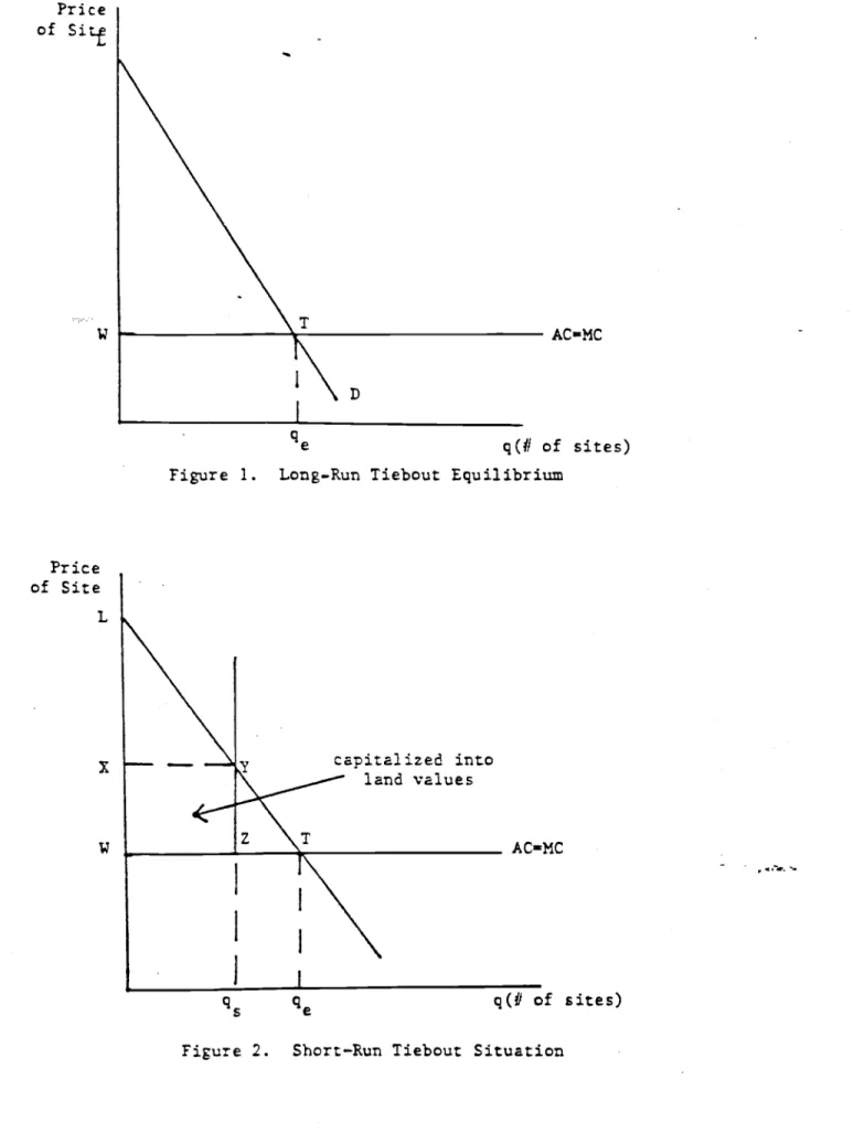
Cities differ by the quality-adjusted amount of the service they provide. To obtain 5A' an individual must occupy a site in jurisdiction A. All sites are identical. For simplicity let construction costs be zero. Figure 1

represents the demand for sites in a single type or class of community, A. The average cost of providing the service is paid through a local property

tax, the only local tax. The tax burden appears as a price to the

residents. Given the assumptions listed above, average cost, marginal cost, and the tax price per site are identical in the long run so the equilibrium at

T is efficient and is the equilibrium number of sites in the type A communities.

Edel and Sciar (19711) correctly point out that there is no capitalization into land value in this situation even with consumer surplus LWT. There are a sufficient number of towns so that any individual can find a site in an

acceptable community with or without service quality 3A• The marginal

consumer is just indifferent between living in this type A community and the next best alternative type community. This person will not be willing to pay more than $W which equals the net present value of the tax burden in a type A

city. No capitalization can occur because that would raise the entry price above $W.

Edel and Sciar (19714) highlight that capitalization is crucially

dependent upon su:ly conditions. In Figure 2, there is a new supply schedule indicating that c-y q5 sites in type A communities are available. Marginal willingness to pay to live in a type A city is now $X per site.

Capitalization res.its ". .

. assuming

prices were set equal to the

average . .

. cos:"

of producing the service SA (Edel and Sclar (19714, p.

91414)). Competitic: to live in one of' the limited type A cities will result in capitalization int: land prices anytime the tax burden is less than the

-5-marginal willingness to pay to live in the city. In this case, the landowners receive the rectangle WXYZ.2

Conceivably, the government could charge a tax price in excess of $W. In the short-run shortage case, assumption (c) on competition does not fully hold. The key distinction is between inter-type and intra-type competition among communities. There is no decrease in the number of types (A, B, C, etc.) of cities available, but there are no longer enough type A cities to

insure intra-type competition sufficient to force those governments to charge no more than $W for the service flow associated with a site in a type A

locality. Inter-type competition among governments only prevents type A communities from charging any more than $X, the highest entry fee attainable before the excess demand for type A cities turns into an excess supply of type A sites.

If for any reason the local government can charge a tax price above $W per site (or lower effective publicly provided goods output), then some of WXYZ in Figure 2 is transferred from landlords to the bureaucracy. For

example, capitalization of the excess return may be into public sector wages rather than land values. P. tax price of $X per site would completely

eliminate capitalization into land values.

Clearly, the absence of tax or spending capitalization in the standard housing price regression does not necessarily imply there is an efficient allocation of local public goods and services as the early tests of the

Tiebout hypothesis have implied. Concomitantly, a decrease in capitalization over time need not signal the approach of efficiency. It may be that changing political forces have allowed the local public bureaucrats to capture the benefits of running a city that is in excess demand. The implications for the

-6-equal utility hypothesis are discussed more fully in the following section which outlines a test for public sector rent seeking.

In general, the extent of capitalization into land values at least

partially depends upon which interest groups can form and possibly combine to split the rents. There are at least three distinct groups—-landlords

(homeowners), bureaucrats, and renters. Each group can try to capture all of any rents for itself or combine with other groups to split the excess

returns. The greater the percentage of residents who are homeowners, the more difficult it will be for bureaucrats or anyone else to capture any of the excess return represented by WXYZ. Still, a majority homeownership group may not be able to prevent any loss of r.ectangle WXYZ. As the public choice

literature has noted, certain revers.ion rules existing in many states may give local bureaucracies strong bargaining power even vis-a-vis a large group of landowners.3 Even in the absence of such special legislated advantages, free— rider problems can prevent a large number of small diverse homeowners from stopping a cohesive public sector bureaucracy from capturing any of WXYZ as long as it is costly to oust the bureaucracy. Additionally, local politics are often complex with multiple issues and candidates involved in the same election. In this situation, voter ignorance in addition to free ridership can prevent a majority group of homeowners from keeping all of WXYZ through land value capitalization.

There certainly is no strong consensus as to the ability of local

bureaucracies (in center cities or residential suburbs) to control spending and/or taxing agendas in order to increase their own utility. Economic theory

and complex gaming problems do not provide a definitive answer. Empirical analysis will have to do this. Romer and Rosenthal's (1979) review of the public choice research concludes that the available evidence did not support

median voter control through the ballot box. If some local public

bureaucracies are able to capture some of the rents associated with a short-run Tiebout disequilibrium situation, then there should be visible effects on the extent of capitalization into land values across jurisdictions.

Section 4: Controlling for Rent—Capturing Bureaucracies in Capitalization Studies

While urban economists have long realized that property value

differentials partially may reflect differences in the cost of providing local public services, they have not been successful in controlling for bureaucratic costs in capitalization studies. This section outlines a new test based on the previous discussion of how introducing a rent-seeking local government sector substantially alters the implications of the standard capitalization tests in the Tiebout literature. At its simplest the model needs to be

expanded to include an additional equation (or equations) in order to be able to generate some measure of successful public sector bureaucracy

rent-seeking. From that part of the estimation the measure of public sector rent capture can then be included in a reduced form land value capitalization equation such as the expanded Oates—type regression in (3),

(3) LV f(t, S, A, H, F, BR) e

where t represents the local tax rate(s), S is the measure of publicly

provided service(, A is a measure of amenities (nearness to downtown or the beach), H is a ve::or of housing stock characteristics, and F is a vector of personal characteristics such as family income, and BR is a measure of' rents

captured by the l::al bureaucracy.

Suppose that a local government is successful at capturing some or all of the rents generat€ by the scarcity of a particular type of community. By

-8-capturing some of the rents we mean that there is an excess of total receipts (from tax, debt, and other sources) over expenditures required to provide the promised services. The proper approach to empirically test for effects on

property values will depend critically on the manner in which the officials choose to consume the economic rents. The most direct way is to increase their total compensation. This can be accomplished through higher wages and/or fringe benefits (i.e., lavish offices, generous expense accounts,

etc.). However, more subtle methods are also possible. For example, they can keep their compensation constant but reduce the effort required for their jobs by engaging in overstaffing.

Unfortunately, each separate method of rent consumption requires a different type of data in order to detect its presence. To our knowledge, sufficient data are not readily available in order to adequately test for rent

consumption through higher fringes or methods such as overstaffing. Data and statistical procedures are available to test whether rents are consumed

through higher wages. Labor economists in particular have examined whether a given public sector employee receives a wage premium relative to a similarly situated worker in the private sector. Researchers such as Smith (1981) have

found that some local government workers (particularly males in larger urban areas) appear to earn substantially more (in nominal and real terms) than similar private sector workers.

Typically, a micro data set on individual wages, personal attributes, and job traits from a cross section of cities is used to estimate a public/private sector wage differential. The simplest approach is to estimate a single wage equation in which a government sector dummy variable is included (e.g., Smith

(1981)). More sophisticated estimation strategies can be employed to deal with problems that arise if public and private sectors comprise distinct labor

markets.5 An average of' the estimated wage premiums received by the local public employees in a jurisdiction would be a proxy for the BR variable in (3).

Assume that such a measure indicates that government wages are higher than expected in a particular community given the wage structure in the private sector. It would not necessarily be the case that local government employees are consuming rents. Other plausible explanations for the

relatively high wages are that these workers have a higher productivity -than is captured by the explanatory variables in the wage regressions but which is observed by the community or that there are unaccounted for disamnenities

associated with the job and/or city. Fortunately, we can discriminate between these possibilities in (3) because the explanations imply distinct effects when the wage measure is added to a land value capitalization regression.

In this respect, it is important to realize that data on services in particular usually are far from ideal in capitalization studies. A standard practice is to use expenditures by type of service to proxy for output of publicly produced goods and services. Not being able to control effectively

for real services provision means the coefficient on BR and the impacts on other coefficients in (3) must be interpreted with care.

The wage rate premium coefficient should differ depending upon the source of the differential. If successful bureaucracy rent-seeking occurs, the

coefficient will be negative, holding taxes and the services proxies

constant. This is because a lower effective level of services is implied from the situation where total tax revenues remain constant while more of those revenues are diverted to public sector wages. Residents have to be

compensated through lower land prices. In contrast, if the higher wages are payments for higher productivity or for some uncontrolled for disamenity,

-10-there is no implicit reduction in effective services provision, with no compensating land price change needed to keep utilities constant across

jurisdictions. Thus, the productivity explanation implies a zero rather than a negative coefficient on the wage premium measure.

Including a control for public sector rent-grabbing should also influence the coefficients on the other fiscal variables. For example, consider the

interpretation of the coefficient on a tax variable when some measure for abnormal wages is not included in the specification. As the tax rate is

increased holding the real services output proxy (or proxies) constant, two possible scenarios arise•. One is that the added tax revenues go to improving genuinely desired services which are not fully picked up by the services

proxies. In this case, there is no reason for land values to change in order to equate the utilities of mobile workers across jurisdictions.

Alternatively, the added revenues could go to (say) increased bureaucratic wages (i.e., the entry price is raised above $W in Figure 2). In this situation, land values would have to fall to compensate residents for the higher tax burden. The coefficient on the tax rate in this situation reflects the combined influences of' these two possibilities.6

Now, consider the effect of including the wage premium measure as an estimate of BR in (3). Assume first that the measure accurately reflects rent consumption and not something such as differential productivity. The

coefficient on the tax rate now more closely reflects the influence of

uncontrolled for changes in real services output and should have a coefficient closer to zero (if the added real services output from the increased taxes are genuinely desired by the population). However, if the wage differential

measure is picking up (say) unobserved productivity differentials, including the variable in the regression should leave the tax coefficient unaffected as

long as the wage differentials are exactly compensating (if the equal utility hypothesis holds, of course). Thus, it should also be possible to

discriminate between the two general explanations for abnormal wages through their impacts on the tax rate coefficients.

Admittedly, the data requirements of this proposed test are

substantial. In addition to the local fiscal information normally used, micro-level wage, demographic, and job-related data on public and private sector workers across a metropolitan area are also needed. However,

-considering

the claims for bureaucracy agenda control in the public choice literature and wage premium findings in public/private labor market studies, future research should work on compiling the data needed to adequately test

for the effects of possible public sector rent capture on local land markets. Unfortunately, we were not able to find or readilydevelop a sufficiently detailed micro data set on workers across jurisdictions within a given urban area to be able to reliably estimate public/private sector wage

differentials. However, we were able to estimate an expanded Oates-type capitalization equation on a cross section of thirty-seven central cities throughout the U.S. This approach does pose some problems such as how to control for interrgional amenity differences not faced in the standard land value capitalizati:r work.7 Interjurisdictional mobility is also a key assumption in our analysis and mobility may not be sufficiently high across widely dispersed c:zies except in the very long run. Consequently, our results can only he viewed as suggestive. Finer intraurban data sets will have to be developed in the future to perform a more powerful test.8

Data on work€s in the thirty-seven cities in our sample came from the May 1977 Current F:ulation Survey (CPS). While the CPS does identify workers residing in the ce:ral city part versus the rest of the SMSA (there are no

other jurisdiction identifiers besides those for major central cities), the limited number of complete observations on public sector employees even in this large data base forced the use of' both central city and non-central city observations when calculating wage differentials.

The wage premium proxy for the BR variable in (3) was calculated by following an estimation strategy used by the authors in another paper (see Tracy and Gyourko (1986)). There we modelled four separate labor

markets—-private nonunion sector, markets—-private union sector, public nonunion sector, and public union sector. The "potential" wage for the th worker in the

population in each of these four labor markets (j 1, 2, 3, 14) is given by

(ha)

in W1

X.181 +

U.1 (private

nonunion)

(14b)

in W12 X2B2 +

u2

(private union)

(Ltc)

in W3 X33 +

_u.3

(public nonunion)

(Ltd)

in W XjhBh +

u

(public union)

where:

_{u —}

N(Oc);

i 1,.. .,N; j 1,2,3,14.

The data vectors are indexed by the type of labor market since the private sector equations contain industry dummy variabies while the public sector equations contain level of government and public sector job

classification dummies. With this formulation, potential returrs for individual characteristics can vary across each labor market.

Individuals are assumed to select which labor market to participate in by choosing the market which maximizes lifetime expected utility. This utility for the individual participating in the th market is modelled as

(5)

I

Z.y. +

. .

i

1,.. .,N

ij 1

)

j 1,2,3,14

-13-Using the indicator function in (5), we proceeded to estimate the wage equation in each market using the generalized two-stage procedure for

switching regressions with an endogenous switching rule discussed in Lee (1982). Consistent estimates are obtained with this procedure.9

The coefficient vectors (6) of the two public sector wage equations generated by the two-stage estimation of (14) and (5) were used to compute the expected wages of individual local public employees in each city (WexP1) as defined in (6),

(6) Wexp. .

8!X.

13 3 13

where i indexes the workers, j 3 (public nonunion sector) or j 11 (public union sector), and and t3 are the same as 63 in (14c) and 614 in (11d) except each contains an added selectivity parameter. These coefficient vectors

include the standard human capital and demographic variables (education, experience, race, sex, marital status, etc.), a cost—of-living index that varies by city,1° regional dummies, dummies by type and level of government worker,11 as well as the selection bias term.

The wage differential for a specific local public employee (Wdif1) is calculated as the difference between the employee's actual wage (Wact1) and his or her expected wage (Wexp) as shown in (7).

(7) Wdif. Wact. .

- Wexp.

ii 1] 13

This differential measures how different are a specific local public

employee's actual wages from what would be expected for that employee in the same job based on the coefficient vector generated using all the public

workers in the sample. For (say) a local police officer in New York City, the measure reflects how different are his or her wages from what a similarly

looking police officer would expect to earn on average throughout all the cities (controlling for cost—of—living differences and broad regional amenities, too).

The estimated public sector wage differential for a city is the average of these individual local public worker differentials in percentage terms. This average is then used as the BR variable in (3) and (8).

The capitalization equation estimated is given in (8),

(8) lnProp

a +

a

1nPTR +

ci 1riLOCINC + a 1nSPENDPRC + a 1nFAMINC79

c 0 1 c 2 c 3 c 14 c

+ a

1nHEAT +

a NEWHOUSE + a

BR +

e

5 e 6 c

7 c

c

where the c subscripts the thirty-seven cities i the sample and the other variables are labelled in the key provided in Table 1.

Column one of Table 2 shows the regression results for (8) without any bureaucratic rents variable. We included both effective property tax rates and wage and/or payroll tax rates to capture the local tax environment. Over one-third of the cities in the sample use a wage or income tax. The local income tax rate has a negative coefficient and is significant at or near the

.10 level. The property tax rate has a small coefficient and is never

significantly different from zero. Residents appear to have to be compensated through lower property prices for higher wage taxes but not for higher

property taxes. Local per capita spending has a significantly positive effect on local property prices. Other variables thought to affect the level of demand such as mean per capita income (FAMINC79) also significantly influence property values in the anticipated direction. An increasing number of heating degree days (HEAT) has a negative but not always highly significant effect on housing values. The percentage of relatively new housing in the city is

included as a control for the quality of the housing stock, and it always has a significantly positive effect on median property value.12

Adding in the wage differential proxy for BR changes virtually none of the regression results in a significant manner as the second column of Table 2 shows. The BR coefficient is negative but it is estimated very imprecisely. These results are not inconsistent with the hypothesis that measured wage differentials reflect primarily unmeasured productivity of public sector workers and that public bureaucracy rent consumption is not significantly

influencing land prices across major cities although we have noted the power of this test may not be very high.

Column three of Table 2 presents the regression results when the wage differential data underlying the BR variable are represented in another form. Instead of using the city averages of (7) directly, a dummy variable for BR was constructed. If the average differential for the city was greater

than one standard deviation above the mean differential for all the cities, then BR was set equal to one. Otherwise, BR was set equal to zero.

We did this for a variety of reasons. First, we suspected that the relatively large measured differentials in some cities were more likely to be indicative of some successful rent capture rather than primarily reflecting unmeasured productivity differences across workers or other noise in the data possibly involving factors such as uncontrolled for amenity differences.

Second, the marginal homeowner may have great difficulty in accurately perceiving whether a relatively small differential represents pure rent consumption by public officials or whether the differential reflects

compensation for scie uncontrolled for productivity or disarnenity associated with the job or city. In a sense, the marginal homeowner has a similar problem to the ecor.ometrician in that not everything can be observed so that

the smaller the differential the more difficult it is to tell whether it is deserved or not. Only large wage differentials may be accurately perceived as rent-grabbing on the part of local public employees.13

Third, we suspected that if local public employees were able to

appropriate some of the excess return arising from a shortage situation, they would not consume the rents solely through higher wages. Some of the excess return may be being consumed through abnormally high nonwage benefits

involving pension plans, sick leave, vacations, etc. Various other nonwage amenities directly enhancing the workplace environment (e.g. plush offices) may also be greater.

vlhen the actual estimated wage differentials from (7) are used in (8), the coefficient on BR reflects solely the influence of the variance in the measured wage differentials across cities. When BR is represented as a 0—1 dummy, its coefficient may reflect other forms of public sector rent

consumption such as higher benefits, plush offices, and the like. If consumption of rents through wages is positively correlated with rent

consumption in other forms, and if nonwage rent consumption is quantitatively important, then this new form of the BR variable will be able to pick up those added influences.

The coefficient on BR in column three is negative and significant at. the .05 level.1 This provides the first indication we are aware of that

potential residents may be being compensated through lower property prices in cities where local public employees earn substantially higher wages than similar local public employees earn on average in other cities.15

The coefficient implies that median property values were depressed by 29 percent in those seven cities with measured wage differentials in excess of

one standard deviation above the sample average differential. 6 The size of this effect in absolute terms is easily calculated in (9) and (10),

(9) IPV —

(.29)IPV

APV or IPV

APV/.71,

where APV is the actual median property value as defined in Table 1, and IPV is the implied median property value in the absence of the rent-grabbing local public employees. Further,

(10)

PV APV —

IPV

with PV being the amount of the estimated decline in median house value. Obviously, the estimation of' (10) is likely to be more accurate the closer is a city's median house value to the overall sample average median value. The full sample mean median house price is $30,775 with a standard deviation of $11,937. There is a wide range in median values among the seven

relatively high wage cities with Detroit having the low value of $18,1142 and Anaheim the high value of $56,589. Median values for 1976 and estimated values of (10) are presented in Table 3. Our further comments are made

primarily with respect to Chicago because it has the APV closest to the sample average APV.

The estimated changes in property value have direct implications on what the level of local public employee rent consumption should be. In order to calculate this value per local public worker, we begin by restating (10) in a different form. We represent the estimated fall in property value as a

perpetuity in (11),

(11) -— Annual Burden of Excess Local Public Wages

i

with (12) following

-18-(12) Annual Burden of Excess Local Public Wages PV*i

This assumes of course that a constant public employee wage premium is expected to persist forever.

To compute (12), we used the Federal Home Loan Bank Board's mortgage yield figure of 9 percent in 1976 as the discount factor i. The units of the

annual burden figure in (12) are a dollar amount per house. To arrive at a dollar amount of rent consumption per local public worker, we need to multiply (12) by the number of houses per local public worker as in (13),

(13) LPWR-- Annual Burden of Excess Local Public Wages Houses

House Local Public Worker

where LPWR is the implied value of local public worker rent consumption. The number of houses per local public worker was computed from information in the 1977 County and City Data Book. The number of equivalent full time local public employees in the city is provided directly. The number of homes was calculated by dividing the city's population by four.

For Chicago, the city closest to the average median housing price among the seven relatively high wage cities, the value of LPWR was approximately $8155. This is 52 percent of the average Chicago local public employee's annual wage income.17 Assuming benefits are approximately one-third of wage income,18 the value of rent consumption for a local public worker in Chicago equalled approximately 39 percent of the total wage-benefit package. While these estimates are high, they are not completely unbelievable. In

particular, they should not readily be interpreted as implying that the wage-benefit package for Chicago city employees would necessarily be 39 percent lower in the absence of any rent-grabbing.19 Such simple ceteris paribus experiments with a wage-benefit package may not be appropriate if everything

—19-else cannot really be held constant. In this respect, it is important to remember that rents may be being consumed in other forms (overstaffing for example) which are picked up in the BR coefficient used to generate PV in (11).

Detroit was the city with the lowest median property value ($18,1142). Its value for LPWR was $8337. This amounted to 147 percent of annual wage income and 35% of' an estimated wage-benefit package. The results on LPWR for Anaheim, the city with the highest median house value among the seven cities, are an order of magnitude too large to be believable. The LPWR value was $50,731. This was 305 percent of annual wage income and 229 percent of wages and benefits. The 29 percent lower median house value implied by the BR coefficient may not be very relevant for Anaheim. Anaheim's observed median house price is in excess of two standard deviations above the sample average median house price. Anaheim is also an outlier in the number of houses per

local public worker. It had almost twenty-four houses per full-time local public employee in 1976 while the average for the other cities was ten.

Additionally, it could just be a statistical quirk of the sample that Anaheim appears as a city with relatively high local public wages.2°

While better local data on jurisdictions in individual metropolitan areas are clearly needed, the results in Table 2 and in footnote 15 do provide the

first empirical evidence that local public sector rent seeking may be influencing prices across land markets. We also believe that our approach provides a sensible way to generate an estimate of public sector rent consumption and that our estimation strategy can effectively discriminate between real rent grabbing and noise in the data.21

-20-Section 5: Further Implications of Public Sector Rent-Seeking in a Tiebout World

If public sector rent grabbing is occurring, it should have important implications for the local regulatory process and, hence, for the political and economic development of a city. There is an interesting political economy of the battle for WXYZ in Figure 2 anytime landowners cannot easily prohibit

others' rent-seeking behavior. Consequently, it is important to realize that the regulatory process can be used in various ways to capture rents or split them with other parties. Indeed, legislated reversion rules have been viewed as a mechanism to prevent homeowners constituting an electoral majority from easily controlling a bureaucracy through the ballot box.

Land use controls are another interesting example. They can be very effective at restricting entry, helping to perpetuate any excess demand condition. Any interest group receiving rents would have an incentive to support adoption of this regulation. Groups not currently capturing rents might also favor such supply restrictions if they believe there is some positive probability that fortunes will change, allowing them to obtain some

of the excess returns in the future.

While land use controls act as barriers to entry, different price—setting regulations such as property tax rate caps and rent controls can be viewed at least partially as rent—splitting devices. Some type of rent-splitting

solution will arise anytime a single group is not able to dominate the other groups and reap all of rectangle WXYZ.

Property tax rate caps could set the price of a site anywhere between $W and $X. If the local public bureaucracy has some monopoly power, possibly due to labor union power or special reversion—type rules fostering agenda control, property tax rate caps may be voted by the residents to restrict bureaucracy

rent-seeking. In Figure 3, tax rates are set so that the site price can rise

no higher than $(X-B). The area XYR(X-B) remains as capitalization into land values while (X-B)RZW is captured by the bureaucracy. It is possible that the local public bureaucracy would even favor imposition of tax rate caps in this shortage situation. This would be the case if the regulation was effective as

insurance against defeat or recall in an election with subsequent loss of all economic rents. The tax rate caps may delineate just what type of rent-splitting will be tolerated by resident landowners. The regulation could be rent-maximizing over the long run for the bureaucracy if it decreases

-uncertainty

about the maximum entry price that can be charged before the landowning electorate is likely to act to prevent any loss of' WXYZ in Figure

3.

Rent controls can serve a similar rent-splitting function. In excess demand situations like that described above, renters and the public

bureaucracy both might favor rent controls. The bureaucracy could offer lower publicly provided services prices to insure against recall along with rent

controls to limit capitalization into land values. In Figure 3, $(X—B) is again the effective tax price of a site in the community with rent controls such that the rental ceiling is equal to the long-run price of housing

services. In this case, the landlords reap none of' the excess return from the shortage but they still will offer housing services in the city because a competitive return is being received. With the site price set at $(X-B), the distance B is the payment (in terms of lower service prices) to residents

(renters in particular) for keeping the bureaucracy in office. Admittedly, this scenario is more likely in the larger more heterogeneous cities with relatively large renter populations.22

Which regulations would appear at any given point in time depends upon the relative bargaining power of the relevant interest groups and the costs of

-22-imposing them. It is beyond the scope of this paper to model in any detail the politics that would allow any specific coalition to arise in order to

impose a given regulation. Rather, this section merely highlights that a broader set of regulatory vehicles are available to rent-seeking bureaucracies

than has previously been investigated in the public choice literature. We suggest that certain increasingly common regulations may have arisen at least partially because of their utility as rent-enhancing or rent-splitting

devices. Additionally, the discussion in this section reemphasizes that-successful bureaucratic rent-seeking further muddles interpretation of land value capitalization in terms of the Tiebout hypothesis. How much of the rectangle WXYZ in Figure 3 represents land value capitalization clearly can be dependent upon the actions of a regulatory body and the attempts by various actors to influence its behavior.

Section 6: Conclusion

Due to slowly adjusting supply conditions and imperfectly flexible

jurisdiction boundaries, localities in metropolitan areas may be in a Tiebout disequilibrium like that discussed in Section 2 for long periods of time. The capitalization literature has implicitly or explicitly assurried that landowners reap all the benefits from such a shortage situation. This need not be the case even in suburbs with little or no absentee landownership. Indeed, researchers in the public choice literature contend that some local public bureaucracies in these suburbs have been able to control budget agendas for their own benefit.

We examined the potential for bureaucracy rent-seeking and its effects on land value capitalization within a standard Tiebout model. There is an

interesting and complex political economy involved in the capturing of

economic rents in a Tiebout disequilibrium that largely has not been discussed

in the literature. An array of regulatory devices including land use

controls, tax rate caps, and rent controls can be used to enlarge and divide economic rents. Further, any successful public sector rent—seeking seriously distorts interpretation of land value capitalization results in terms of the Tiebout hypothesis. More sophisticated tests of the Tiebout hypothesis such as that suggested by Epple, Visscher, and Zelenitz (1978) will have to account for the added complications of public sector rent-seeking highlighted here.

Finally, a new approach to test for the presence of bureaucracy rent-seeking was proposed. The test involved an expanded Oates-type capitalization

regression. The test exploits the fact that such rent-seeking should have identifiable effects on land value capitalization assuming mobility is high enough that a given individual can achieve equal utility in any locality within some urban area. Although Epple and Zelenitz (1981) have pointed out that the Oates regression generally does not adequately test the Tiebout hypothesis, our expanded version could do so in certain instances. If the rent-capturing proxies were significant, then we would know that public services were not being efficiently provided. However, an insignificant effect for the rent-capturing proxy would not necessarily imply that the Tiebout propositions truly were operating.

Our results indicated that, even across major cities, differences in successful rent capture by local public employees affected property prices. We think the results strongly imply that further work needs to be done in this area. In particular, data need to be found to perform a similar study across jurisdictions within a single well—defined urban area. Also, different groups of public workers may have different rent capturing abilities. Future work should attempt to determine whether this is the case, and if so, why it is the

case. Information such as this may help explain why certain localities suffer from rent—grabbing public sectors while other jurisdictions do not.

—25-Footnotes

1See Rose-Ackerman (1983) for a thorough review of and bibliography on these literatures.

2Absentee landlords typically are assumed to eliminate complications from income effects. Competition among potential residents raises rent bids until the sum of the rent plus tax costs just equals the marginal willingness to pay to enter (all in per unit of the service terms). Land value rises because it is the discounted value of the rent payments stream.

3See Romer and Rosenthal (1979) and Denzau and Grier (19814) for more details on reversion rules and their effects on local school expenditures.

14See Ehrenberg and Schwarz (1983) for a complete review of research on public sector labor markets and how they appear to differ from private sector markets.

5me single wage equation approach assumes that personal attributes such as education and experience have the same return in the public and private

sectors. This need not be true if these are distinct labor markets. Additionally, the choice of labor market may not be exogenous. If self-selection is not controlled for, wage regression coefficients can be biased. These and other econometric problems can be addressed by employing the

switching regression framework with an endogenous switching rule. Lee (1978, 1982) and Maddala (1983) provide outlines of the more advanced techniques.

6The services coefficients reflect similar combined references, too. We do not go into that story for space reasons. Furtner, we are assuming

balanced budgets with no debt financing or intergovernmental grants--typical underlying assumptions in empirical studies of capitalization. Our

interpretation is an example of the point made by Linneman (1978) that tax (and spending) coefficients almost certainly represent more than just

-26-capitalization of'

tax

_{(or spending) differentials across jurisdictions. If} intergovernmental revenues are also a relevant omitted variable, then the tax coefficient would also reflect differences in local grantsmanship abilities to some extent.

7See Leeds (1985) for a critique of Tiebout-type studies that use interregional rather than intraregional data.

8The power is low for the null hypothesis that there is successful local public sector rent seeking and residents are compensated for this through lower property prices. While a rejection of the null may not convey important information, any findings in support of the null hypothesis would be

especially encouraging given that the coefficient on BR in (3) probably is biased towards zero because of our use of an interrnetropolitan city data base.

9See Tracy and Gyourko (1986, pp. 9—12) for a complete description of the implementation of the two-stage procedure.

10The cost—of-living index is from the Bureau of Labor Statistics (BLS) intermediate family budget data across metropolitan areas in the U.S. If direct budget data was not available for a particular city, budget data from a nearby city was substituted.

11Local public employees are distinguished from state and federal employees in the data. At the local public level, teachers and policemen— firemen are further distinguished from all other local public sector workers.

12We experimented with various small _{changes in the specification. For} example, we included the percentage population change in the city from 1970 to

1980 to help control for demand shifts. The variable had a significantly positive coefficient as expected. However, this variable turns out to be fairly highly correlated with the level of family income across our cities. Including the population change variable significantly weakens the family

-27-income effect without substantially affecting the other coefficients. Neither this nor other similar specifications yielded results significantly different from those reported in Table 2. Due primarily to the small sample size, we attempted to keep the specification as parsimonious as possible and report only (8) in Table 2.

13Bergstrom, Rubinfeld, and Shapiro (1982) provide some evidence that individuals do have trouble making fine distinctions about differences between desired and actual public spending levels. Those authors had qualitative response data from surveys on whether Michigan residents desired more, less, or about the same level of spending on public education as currently existed

in their districts. Bergstrom, Rubinfeld, and Shapiro questioned whether respondents could accurately determine whether they truly desired more or less public spending if their desired amounts were only slightly more or slightly

less than the actual amount of spending taking place. They structured their estimation so that they could solve this problem. They determined that

desired spending would have had to have been 1.5 times actual spending for an individual to express a preference for more spending. In a similar vein, it may be that a prospective resident cannot accurately discriminate between a

deserved wage premium and undeserved rent grabbing if the observed differential is not somewhat of an outlier.

1We also ran a specification with the measured differential and its

square entered on the right-hand side. Both coefficients were insignificantly different from zero.

5Four of the smaller cities in the sample (Akron, Albany, Columbus, and Greensboro) had oniy four or five usable observations on local public

employees. Note that three of the four cities rank as having the smallest or near the smallest measured average wage differentials. (See the table in the

-28-Appendix.) There is a greater probability for these cities than for the

others that the measured differentials do not accurately reflect the true mean wage differential for local public employees in the relevant city. We

included these cities in the regressions reported in Table 2 because we were worried about losing variance in the other variables since we started with a relatively small sample size. Further, we do not know for sure that these cities' differentials are substantially inaccurate.

Nevertheless, we did redo the regressions in Table 2 after dropping these four cities. Thirty-three cities remained. Rerunning the specification in column two yielded an estimated BR coefficient and standard error of -0.07 and 0.141, respectively. When BR is represented as a 0—i dummy as in column three, the coefficient and standard error based on the smaller sample were -0.26 and 0.12, respectively. Other coefficients were generally not materially affected either.

l6This is arrived at by following the algorithm suggested by Halvorsen and Palmquist (1950) for adjusting dummy variable coefficients in

semilogarithmic ec..ations. The implied percentage difference in land values is given by 100(ex:(ci7) — 1) where is the coefficient on BR in (8) when BR is represented as a 0 — 1 _dummy.

17Frorn the CF. data, we calculated the average _{wage across the Chicago} local public workers in the sample. Annual wage income was computed assuming the employee was paid for working 140 hours per week throughout the year or for 2080 hours.

18Zax (1983, ;85) provides evidence that various benefits (pension, medical, miscellar.3us) do comprise one-third or more of wage income of local public employees.

19However, our estimated public-private wage differential for Chicago local public employees was 30.3 percent.

20Results for most of the other cities were sensible and similar to those reported for Chicago and Detroit. The only exception was St. Petersburg where the LPWR figure was again unbelievably high. It amounted to almost 90 percent of wages and benefits. Baltimore had the smallest absolute and percentage LPWR effect. Its LPWR figure was $1421114 and was only 20% of annual wage income

plus benefits.

is worth noting that we calculated the wage premium measure in another way, too. We began by simply estimating via OLS two semi-log wage equations across workers in each city in the sample.

(9)lnwage. B +X. +BDOC.

+BU. +BR.

+CLI. +

i,pr

0 1 i,pr 2 _1,pr 3 i,pr 14 i,pr 5 i,pr

e. ,

i1,

. . . rn i,pr

(10) ln Wage 8' +

8'X.

+ B'DOC. +

B'U.

+

B'R.

+8'CLI. +

j,pu

0 1 j,pu 2 _j,pu 3 j,pu 14 i,pu 5 i,pu e. ,

j1,

.

. .,n

pu

where i and j subscript individual worker observations, pr and pu denote the public and private sectors, respectively, X is a vector of the standard worker

traits normally used (e.g., age, race, sex, marital status, experience, education), DOC are detailed occupation dummies from the CPS, U is a union dummy variable, R :s a vector of region dummies, CLI is the cost—of-living index for each city. and e is the mean zero error term, and the Bs and 8'S are coefficients or coefficient vectors.

Public/private sector wage differentials were then calculated. A public sector worker in a given detailed occupation was matched into as similar an occupation as possi:e in the private sector. There were some problems with

'-30-matching specific public sector employees to detailed occupations in the private sector. For example, policemen were assigned to the private sector occupation "Protective Services." That occupation covers building security

jobs which are not as hazardous as police work. This inability to fully control for job-related differences in the matching process adds noise to the calculated wage differentials and is a major reason we report the results based on the other differentials.

An expected wage in the private sector for a specific local public -employee was then computed using the private sector coefficient vectors (the Bs). The individual's wage differential is the actual wage received by the local public employee minus his/her expected wage in a similar private sector job. A city's wage differential is the average of the individual public worker differentials in percentage terms. This average was then used as the BR variable.

The coefficient and standard error on this version of the BR variable were —0.09 and O.10, respectively. We also constructed the BR variable as a 0 - 1 dummy in the same manner as with the other wage premium measure. The coefficient and standard error on this version of the BR variable were -0.12 and 0.12, respectively.

When the four small cities with very few local public worker observations are dropped from the sample and the regressions rerun on the smaller sample,

the results were not significantly changed.

is even conceivable that landowners would favor rent controls as a rent splitting device although some extreme assumptions need to be imposed. An earlier version of this paper contained a detailed example. It can be summarized in terms of Figure 3. The case was for a city where all

landownership was absentee. Note that since $X is the true willingness to pay

for a site, competition among potential residents guarantees that $X is what will be paid ultimately. In this case, landowners cannot credibly convince

renters it is worthwhile to prevent the public bureaucracy from raising the site price. If landlords were willing to make side payments of' $B to renters if the government is recalled, the full entry price to the city would fall to $(X—B). As long as there is excess demand there will always be potential residents bidding the entry price back up to $X by rebating the side payment

back through higher rents.

-Stringent

temporary rent controls which also prohibit cash side payment schemes such as key money could actually benefit landlords in this

situation. With a mandated rent control ceiling of ${(X-B)-W}, voting renters would have an Incentive to force the bureaucracy to set an entry price of

$W. Residents will still pay $X to live in the city, but the rent control prevents full payment from being in cash. Nonmonetary payments represented by the distance B in Figure 3 will be made, with voting to prevent the

bureaucracy from raising tax rates or cutting service levels one important example of such payment. Capitalization into land values is represented by

the smaller rectangle W(X-B)RZ. Landlords have to trade off some of the potential short-run gain in the form of lower housing prices because renters are incurring, some nonmonetary costs to live in the city.

The beneficial aspects of rent controls to landlords arise in this case because they could not otherwise credibly persuade the resident renters it was

in their interest to restrain the bureaucracy. While a contrived example, this case and the ones outlined in the text further indicate the various possible uses of price-setting rules as rent-splitting devices for different factions in a metropolitan area not in full Tiebout equilibrium. The

durability of rent controls in the U.S. in the face of their obvious high

-32-costs may well be due to the fact that various groups, not just a single group of renters, benefit from the regulation.

References

Bergstrom, T., Rubinfeld, D., and Shapiro, P., "Micro-Based Estimates of Demand Functions for Local School Expenditures," Econornetrica 50, no. 5,

(1982): 1183—1205

Denzau, A. and Grier, K., "Determinants of Local School Spending: Some Consistent Estimates," Public Choice 1414,

no.

2 (1984): 375-384. Edel, Matthew, and Sciar, Elliot, "Taxes, Spending, and Property Values:

Supply Adjustment in a Tiebout-Oates Model," Journal of Political Economy 82, no. 5 (September/October 19714): 9141_54.

Epple, Dennis, and Zelenitz, Allen, "The Implications of Competition Among

Jurisdictions:

Does Tiebout Need Politics?" Journal of Political

Economy 89: 1197—1217.

Ehrenberg, R. and J. Schwarz, "Public Sector Labor Markets," National Bureau of Economic Research, Working Paper No. 1179, August 1983.

Epple, Dennis, Zelenitz, Allan, and Visscher, Michael, "A Search for Testable Implications of the Tiebout Hypothesis," Journal of Political Economy 86, no. 3 (June 1978): 405—25.

Henderson, 3.

Vernon,

"The Tiebout Model: Bring Back the Entrepreneurs," Journal of Political Economy 93, no. 2 (April 1985): 2148—264.

Inman, Robert P., "Public Employee Pensions and the Local Labor Budget," Journal of Public Economics 19 (1982): 149_71.

Leeds, Michael A., "Property Values and Pension Underfunding in the Local Public Sector," Journal of Urban Economics 18, no. 1 (1985): 34_146.

Linnernan,

Peter, "The Capitalization of Local Taxes: A Note on Specification," Journal of Political Economy 86 (1978) 535-8.

Maddala, G. S., Limited-Dependent arid

Qualitative

Variables in Econometrics. Cambridge University Press, Cambridge, 1983.

Meadows, George R., "Taxes, Spending, and Property Values: A Comment and Further Results," Journal of Political Economy 814, no. 14 (1976): 869— 880.

Niskanen, William, "Bureaucrats and Politicians," Journal of Law and Economics (December 1975).

Oates, Wallace, "The Effects of Property Taxes and Local Public Spending on Property Values: An Empirical Study of Tax Capitalization and the Tiebout Hypothesis," Journal of Political Economy 77, no. 6

-(November/December 1969): 957-71.

Romer, Thomas and Rosenthal, Howard, "Bureaucrats Versus Voters: On the Political Economy of Resource Allocation by Direct Democracy," Quarterly Journal of Economics (November 1979): 563-587.

__________ "The Elusive Median Voter," Journal of Public Economics 12 (1979): 1143—170.

Rose-Ackerman, Susan, "Beyond Tiebout: Modeling the Political Economy of Local Government," in Local Provision of Public Services: The Tiebout Model after Twenty-Five Years (George Zodrow, editor). New York:

Academic Press, 1983.

Rosen, Harvey and Fullerton, David, "A Note on Local Tax Rates, Public Benefit Levels, and Property Values," Journal of Political Economy 85, no. 2

(1977): 1433...1414O.

Sarnuelson,

Paul, "A Pure Theory of Public Expenditure," Review of Economics and Statistics 36, (November 19514): 387-9.

Smith, Sharon P., "Public/Private Wage Differentials in Metropolitan Areas," in Public Sector Labor Markets, Peter Mireszkowski and George Peterson (eds.), The Urban Institute, 1981, 81-103.

-35-Tax Foundation, Inc., Facts and Figures on Government Finances, New York: -35-Tax Foundation, Inc., 1978.

Tiebout, Charles M., "A Pure Theory of Local Expenditures," Journal of Political Econçy 65, no. 5 (October 1956): )416_214.

Tracy, J. and Gyourko, J., "An Analysis of Public and Private Sector Wages Allowing for Endogenous Choices of Both Government and Union Status"

(February 1986), discussion paper.

U.S. Bureau of the Census, Census of Governments, Washington, D.C.: GPO, Vol. II, 1977.

_________

County

and City Data Book, Washington, D.C.: GPO, 1977 and 1983. Zax, Jeffrey, S., "Labor Relations, Wages and Nonwage Compensation in

Municipal Employment," NBER Working Paper, No. 1582, March 1985.

_________

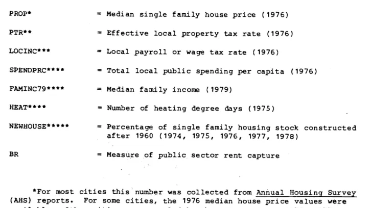
"Nonwage Compensation: Past Growth and Future Prospects," Discussion Paper, Harvard University, April 1983.

Table 1: Variable Key

PROP* _{Median single family house price (1976)} PTR** =

Effective

_{local property tax rate (1976)} LOCINC*** =

Local

_{payroll or wage tax rate (1976)}

SPENDPRC**** =

_Total

_{local public spending per}

_capita

₍₁₉₇₆₎ FAMINC79**** = Median family incon (1979)

HEAT**** = Nunther of heating degree days (1975)

-NEWHOt.JSE***** =

_Percentage

_{of single family housing stock constructed} after 1960 (1974, 1975, 1976, 1977, 1978)

BR = _{Measure of public sector rent capture}

*For most cities this nunber was collected from Annual Housing Survey (AklS) reports. For some cities, the 1976 median house price values were available. Other cities were sampled by the AHS in either 1975, 1977, or 1978. Values for those cities were adjusted by the change in the Home Purchase Price component of the Consumer Price Index (CPI) over the

appropriate time period to estimate what the median price would have been in 1976. Four of the cities in the sample (Akron, Gary, Greensboro, and St. Petersburg) were never surveyed in the AIlS. We calculated median house value for 1976 based on 1970 and 1980 values reported in the 1977 and 1983 issues of the County and City Data Book. We assumed a constant rate of change in value beginning with the 1970 price which would yield the published 1980 value.

**The effective property tax rate is for the central city (not the overall SMSA) and is a nominal rate corrected for by the local assessment— sales ratio. These data are from Volume II of the Census of Governments for 1976.

***Local payroll or wage taxes for the central city were collected from Facts and Figures on Government Finances published by the Tax Foundation.

****These variables were collected from issues of the County and City Data Book. They are for the central city only (although the distinction from

the entire SMSA is irrelevant for the IAT variable).

*****Data for this variable were collected from various years of the Annual Housing Survey (AIlS) and the County and City Data Book. The specific year used for each city depended upon whether the city was included in the AHS, arid if so, in what year.

Table 2: Capitalization Regressions

Dependent Variable: Lri Median House Value (1976)

Independent (1) (2) (3) Variables Intercept 0.73 0.31 —0.92 (3.68) (3.76) (3.41) Lii PTR 0.05 0.06 0.08 (0.07) (0.08) (0.07) Ln LOCINC —0.16 _0.17* _0.15* (0.09) (0.09) (0.08) Ln SPENDPRC 0.29** 0.32** 0.38** (0.12) (0.12) (0.11) Lii FAMINC79 0.75** 0.78** 0.93** (0.35) (0.36) (0.33) Lii HEAT —0.05 —0.06

-0.10

(0.05) (0.05) (0.05) NEWNOUSE

0.01*

0.01

0.01

(0.003) (0.004) (0.003) BR —0.27 _0.34** (0.39) (0.13) R2 0.34 0.33 0.45 F 4.05 3.48 5.17 PROB > F .0043 .0079 .0007

Note: Standard errors in parentheses

**

_denotes

sigiiificance at .05 level

Table 3: Estimates of Effects on Property Value Ariahei m Denver Chicago Baltimore Detroit Rochester St. Petersburg $56 ,

589*

33,300 31,689 21,300 18, 142** 20,881 24,107 —$23, 114 —13,601 —12 ,943 —

_8,700

— _7,410 —

_8,528

—

_9,846

* More

than two

standard

deviations above the overall sample mean. **More than one standard deviation below the overall sample mean.

APV

Median

House

PV

Appendix: City Rankings by Measured Wage Differential (Largest Differential Receives Highest Ranking)

Cit Average Public Sector Wage

Premium Rankings Birmingham 25 Anaheim 3* Los Angeles 10 Sacramento 8.5 San Bernadino 36 San Diego 20 San Francisco 17 Denver 4* Atlanta 16 Chicago 7* Indianapolis 28 New Orleans 19 Baltimore 6* Boston 23 Detroit 3* Minneapolis 15 Kansas City 32 St. Louis 18 Newark 31 Albany 8.5 Buffalo 24

New York City 13.5

Rochester 2* Cincinnati 21 Cleveland 26 Columbus Portland 27 Philadelphia 22 Pittsburgh 11 Houston 12 Seattle 30 Milwaukee 33 Miami. 13.5 Akron 37 Greensboro 29 St. Petersburg 1* Gary 35

Note: A ''

indicates

the measured differential is in excess of one standard deviation above the mean differential across all cities in the

sample. The starred cities have codings of when the wage

Price of Site

L

Figure 2. Short—Run Tiebout Situation Price of w T Figure 1.

ACMC

q(/ of sites) Long-Run Tiebout Equilibrium

x

V capitalized into land values AC-MC qO of sites)

Price of Site

x—

AC-MC

q qU/ of sites)

Figure 3. Division of Capitalization Proceeds

Y