Copyright by
Sean Stephen Bader 2018
The Thesis committee for Sean Stephen Bader
Certifies that this is the approved version of the following thesis:
Seismic and well log data integration using data-matching
techniques
APPROVED BY
SUPERVISING COMMITTEE:
Sergey B. Fomel, Supervisor Kyle T. Spikes
Seismic and well log data integration using data-matching
techniques
by
Sean Stephen Bader
THESIS
Presented to the Faculty of the Graduate School of The University of Texas at Austin
in Partial Fulfillment of the Requirements
for the Degree of
Master of Science in Geological Sciences
THE UNIVERSITY OF TEXAS AT AUSTIN May 2018
Dedicated to my parents and grandparents who supported my education and provided encouragement over the years
Acknowledgments
I owe a great deal of gratitude to Dr. Sergey Fomel. He has provided me with the opportunity to continue my education in geophysics which is one of the most chal-lenging, unique, and interesting fields of study. Sergey’s insight and understanding of the theory and application of challenging geophysical concepts is unparalleled and has pushed me to broaden my horizons and understand the connections between concepts which I had thought were completely unrelated. He has allowed me the freedom to explore topics that I found interesting, and we tackled several fun and unique projects. I greatly appreciate everything Sergey has taught me during my time in Austin.
The work discussed in this thesis is an accumulation of several collaborations and publications. Each chapter is pieced together from the following works: Bader et al. (2017), Bader et al. (2018a), Bader et al. (2018b), Bader et al. (2018c), and Bader et al. (2018d). I am very thankful to the co-authors on these works in particular for their assistance and input on the projects.
The Texas Consortium for Computation Seismology (TCCS) has been home to me for the last two years, and the members of this group are kind, supportive and unbelievably hard working. I am very thankful to past and present members of the group that I have the opportunity to work with: Dr. Xinming Wu, Dr. Zhiguang Xue, Dr. Yanadet Sripanich, Dmitry Merzlikin, Yunzhi Shi, Mason Phillips, Luke Decker, Yunan Yang, Ben Gremillion, Zhicheng Geng, Harpreet Kaur, and Nam Pham. I also appreciate the financial support and insights provided by the sponsors of TCCS.
processing and imaging techniques and the daily morning coffee. I also would like to thank Philip Guerrero who supports all of the geoscience graduate students at UT Austin. I appreciate the members of my committee, Kyle Spikes and Carlos Torres-Verd´ın for their feedback and recommendations on the work presented in this thesis.
Also, I am thankful for the many people whom I have had the opportunity to interact and work with since I started out at Colorado School of Mines, CO. During my undergraduate studies was unbelievably lucky to be surrounded by a group of friends and professors who are passionate about geology and geophysics and driven to succeed. I am especially thankful to Dr. Terence Young for introducing me to the field of geophysics; I would not have taken up this line of work without the guidance and support from him. Also, I want to thank Dr. Paul Sava and Dr. Thomas Davis who introduced me to the complexities of real-world problems in geophysics, and whose sense of humor reminded me to have fun solving these seemingly impossible problems.
I would also like to thank my sixth-grade teacher, Anne McIntosh, who intro-duced our class to higher levels of math and science that most elementary students do not get access to until later stages of school. Her approach to teaching and sense of humor set me up for many years of success.
I am very thankful to my grandparents, aunts, uncles and cousins who attended my various academic and sporting events confident that I will do great things. Of course, I might have gotten lost along the way if it were not for my Uncle Nate’s multiple, lengthy, lectures about life in the car rides between Denver and Vail. Finally, I am deeply grateful to my loving parents, Marci and Jerry Bader, for their unwavering
support. Their love and constant encouragement pushed me to achieve new heights. And, last but not least, I am grateful for my siblings, Samantha and Andy, for putting up with me over the years.
Seismic and well log data integration using data-matching
techniques
Sean Stephen Bader, M.S.Geo.Sci. The University of Texas at Austin, 2018
Supervisor: Sergey B. Fomel
Relating well log data to seismic data is an important step in integrated reser-voir characterization studies. Traditionally, an interpreter uses well log data, which has high vertical resolution but little lateral coverage, to understand amplitude vari-ations in seismic data, which has lower vertical resolution than well logs but high spatial coverage. The process of calibration is referred to as a seismic-well tie.
Several problems arise with the assumptions of conventional seismic-well tie workflows. The seismic-well tie involves generating a reflectivity series from available sonic and density logs acquired at the well, which inherently assumes all wells have a sonic and density log available along the entire length of the well. In many cases, this assumption is not valid as the number of wells drilled often out-numbers the number of sonic and density logs acquired. Common procedures to account for miss-ing well logs in seismic-well ties are to use a time-depth relationship from a nearby well or use an empirical relationship to estimate the missing well log from an
avail-able well log. These methods provide constructive solutions. However, variations in structure, stratigraphy or missing/incomplete well logs can result in inaccurate seismic-well ties. In this thesis, I propose a method that predicts missing well log data by first estimating the shifts that align well logs with a reference type log. Once in this stratigraphically correlated, or ‘relative geologic time,’ domain, I interpolate the missing well log data from available logs of the same type. The resulting well log is consistent with available well data and is not distorted by structural or strati-graphic variations. Once complete well log suites are estimated for each well, I focus on improving the efficiency and consistency of multiple seismic-well ties.
The seismic-well tie typically involves a subjective and labor-intensive work-flow that depends on the interpreter’s experience and intuition. I introduce an au-tomatic workflow using local similarity to match the synthetic with the real seismic trace. The advantage of using local similarity to compute the seismic-well tie is that consistent, repeatable, seismic-well ties are achieved. I generate a global log prop-erty volume by interpolating log data along local seismic structure and perform blind well tests to verify the accuracy and consistency of seismic-well ties. I apply this workflow to a 3D seismic dataset with 26 wells and achieve consistent, accurate and reproducible seismic-well ties.
Combining the results of the well log interpolation and seismic-well tie I can generate a time-to-depth relationship for each well regardless of the initial well log suite. As a result, it is possible to generate log property volumes that integrate the high spatial coverage of seismic data with information from well log data.
Well log data can also provide a useful source of information during velocity model building for depth migration. Using concepts and workflows described
previ-ously, I show that the mis-tie between a modeled synthetic and real seismic trace is related to an inaccurate migration velocity. Furthermore, this information can be used to update the migration velocity model such that modeled synthetic seismograms, the seismic image, migration velocities and well log velocities become consistent.
Table of Contents
Acknowledgments v
Abstract viii
List of Figures xii
Chapter 1. Introduction 1
Chapter 2. Review 6
Chapter 3. Missing Log Data Estimation 27
Chapter 4. Seismic-Well Ties 50
Chapter 5. Validation of Technique 69
Chapter 6. Seismic-Well Tie Velocity Update 76
Chapter 7. Conclusions 88
Chapter 8. Appendix 92
Bibliography 98
List of Figures
2.1 Example estimating impedance and reflectivity from well log data. The velocity and density data are from the Penobscot L-30 well offshore Nova Scotia, Canada. . . 9 2.2 Example estimating a time-to-depth relationship using a well log
ve-locity profile. Reflectivity in depth is interpolated to time using the time-to-depth relationship and convolved with a 25Hz Ricker wavelet to generate a synthetic seismogram. The velocity and density data are from the Penobscot L-30 well offshore Nova Scotia, Canada. . . 10 2.3 Synthetic seismogram modeled from well log data overlaying seismic
amplitude data. The velocity and density data are from the Penobscot L-30 well and seismic data are from a dataset offshore Nova Scotia, Canada. . . 11 2.4 Example using linear interpolation to fill in the missing sonic log data.
Using the resulting sonic log, a synthetic seismogram can be modeled; however, a gap is present due to the missing sonic log, which may make it challenging to relate to the available seismic data. . . 14 2.5 Crossplot of velocity and density log data from the Penobscot L-30 well.
Using Gardner’s Equation, I relate the available sonic and density log data assuming α = 0.23 and β = 0.25 for the entire well. . . 15 2.6 Example using Gardner’s Equation to fill in the missing sonic log data.
Using the resulting sonic log, a synthetic seismogram can be modeled that might be a better representation of the subsurface at that location and does not have a gap due to missing information. . . 16 2.7 Reflectivity series in time (left) convolved with a 30Hz Ricker wavelet
to model a seismogram (right). . . 23 2.8 Modeled seismogram (left), modeled seismogram shifted by 40ms
(mid-dle), re-aligned seismogram using the shifts estimated from the local similarity scan (right). . . 23 2.9 Similarity scan and picked optimal shifts (white curve). Warm colors
represent high similarity whereas cool colors represent low similarity. 24 2.10 Noisy reference trace (left), modeled seismogram shifted by 40ms
(mid-dle), re-aligned seismogram using the shifts estimated from the local similarity scan (right). . . 24 2.11 Similarity scan and picked optimal shifts (white curve). Warm colors
3.1 (a) Median filtered gamma log from the reference well (red) and median filtered gamma log from a second well (black). (b) Sonic log from the reference well (red) and sonic log from a second well (black). . . 32 3.2 (a) Median filtered gamma log from the reference well (red) and an
aligned gamma log from a second well (black) after applying estimated alignment shifts. (b) Sonic log from the reference well (red) and an aligned sonic log from a second well (black) after applying estimated alignment shifts from matching gamma logs. . . 33 3.3 (a) Real sonic log cross plotted against the sonic log estimated using
Reverse Gardner equation. (b) Real sonic log cross plotted against the sonic log estimated using the proposed approach. . . 35 3.4 I perform a blind well test by estimating a sonic log using the proposed
approach and comparing the result against the real sonic log. Real sonic log (black) versus estimated sonic log (blue) along two 1600ft intervals along the reference log. . . 36 3.5 (a) RMS error between real and predicted sonic logs given all wells in
the dataset and values. (b) RMS error between real and predicted density logs given all wells in the dataset and values. . . 37 3.6 (a) Normalized combined sonic and density RMS error given all wells
in the dataset andvalues. (b) Normalized combined sonic and density RMS error given all wells in the dataset and caliper weighting values. 38 3.7 (a) Original sonic log (black) versus estimated sonic log (blue). (b)
Original density log (black) versus estimated density log (blue). The original well log data is used in the inversion so areas where sonic or density data is available the estimated logs match the original data. In the interval between 3500 ft and 3900 ft, there is a significant deviation in the (c) caliper log indicating an inaccurate measurement; therefore, the estimated log deviates significantly from the original log. . . 39 3.8 (a) Sonic and density bivariate prior distribution at one depth. (b)
Density and total porosity bivariate prior distribution at one depth. (c) Sonic and total porosity bivariate prior distribution at one depth. The sonic log value is interpolated using the method described previously and has higher uncertainty as compared to well logs acquired at the well. 45 3.9 (a) Bivariate likelihood distribution (contours) for sonic and density
well log data in one stratigraphic interval. (b) Bivariate likelihood dis-tribution (contours) for density and total porosity well log data in one stratigraphic interval. (c) Bivariate likelihood distribution (contours) for sonic and total porosity well log data in one stratigraphic interval. Actual well log data (black dots) in one stratigraphic interval. The red line is an empirical estimation Equations 3.8, 3.9, and 3.10. . . 46 3.10 (a) A priori sonic log (blue) estimated from available sonic logs in
the dataset and (b) posterior sonic log estimated using the proposed approach (blue). Each estimated sonic log is compared against the real sonic log (black). . . 48
3.11 (a) Real sonic log cross plotted against the a priori sonic log. (b) Real sonic log cross plotted against the maximum a posteriori sonic log estimated using the proposed approach. There is a subtle improvement using the proposed approach . . . 49 4.1 Synthetic modeled using the initial sonic log (green). Closest trace to
the well location extracted from the phase adjusted seismic data (black). 52 4.2 Similarity scan between the modeled synthetic seismogram and the real
seismic trace. The warm colors indicate high similarity (high correla-tion) between the synthetic seismogram and real seismic trace whereas the cold colors indicate low similarity (high correlation) between the synthetic seismogram and real seismic trace. . . 53 4.3 Synthetic modeled using the initial sonic log (green). Synthetic
mod-eled using the sonic log updated after one iterations of matching using LSIM to estimate shifts (red). Closest trace to the well location ex-tracted from the phase adjusted seismic data (black). . . 54 4.4 Similarity scan between the modeled synthetic seismogram and the real
seismic trace. The warm colors indicate high similarity (high correla-tion) between the synthetic seismogram and real seismic trace while the cold colors indicate low similarity (high correlation) between the synthetic seismogram and real seismic trace. Notice high similarity values aligned along zero relative shift indicating no shifts are required to align the synthetic seismogram with the seismic trace. . . 55 4.5 Initial sonic log (green). Updated sonic log using the shifts estimated
from LSIM to align the synthetic seismogram and real seismic trace (red). . . 58 4.6 Similarity scan between the modeled synthetic seismogram and the real
seismic trace. Smoothing is reduced by 80% as compared to Figure 4.2. Notice the oscillatory behavior in the pick from the similarity scan. . 59 4.7 Initial sonic log (green). Updated sonic log using the shifts estimated
from LSIM (Figure 4.6) to align the synthetic seismogram and real seismic trace (red). Notice that the oscillatory behavior in the shift pick from LSIM results in a significant difference between the original and updated well sonic log. . . 60 4.8 Similarity scan between the modeled synthetic seismogram and the real
seismic trace weighted by the energy of the synthetic seismogram and seismic trace. Smoothing is reduced by 80% as compared to Figure 4.2. Notice the pick from the similarity scan matches the areas of high similarity. . . 61 4.9 Initial sonic log (green). Updated sonic log using the shifts estimated
from LSIM (Figure 4.8) to align the synthetic seismogram and real seismic trace (red). . . 62 4.10 Statistical wavelet extracted from the Teapot Dome seismic dataset. . 65
4.11 Synthetic modeled using the initial sonic log (green). Synthetic mod-eled using the sonic log updated after four iterations of matching using LSIM to estimate shifts (red). Closest trace to the well location ex-tracted from the phase adjusted seismic data (black). . . 66 4.12 (a) Initial sonic log after Backus averaging (green). Updated sonic log
after four iterations of matching using LSIM to estimate shifts (red). Initial sonic log after interpolation of missing data (black). (b) Initial TDR (green). Updated TDR after four iterations of matching using LSIM to estimate shifts (red). . . 67 4.13 Seismic crossline through well in Figures 4.11 and 4.12. I observe a
good tie between the modeled synthetic and real seismic data. The sonic and density logs used to model the synthetic are estimated using the proposed approach. . . 68 5.1 Time slice through seismic data at 0.72 seconds. The stars indicate
the location of each well. The purple well is used as the reference well for missing log data interpolation. . . 70 5.2 (a) Phase adjusted seismic amplitude data. (b) Inline dip and (c)
Crossline dip estimated using plane-wave destruction filters. . . 71 5.3 (a) Interpolated sonic and (b) interpolated density based on logs from
26 wells and the interpolant described in Equation 2.11. Note that the interpolated log data follows the seismic structure. . . 72 5.4 Predicted (green) and actual (black) sonic logs from two different wells
using a blind well test. The predicted and actual sonic logs match along the entire length of the well log indicating consistency in seismic well ties. . . 74 5.5 Real sonic log cross plotted against the predicted sonic log from the
blind well test for all 26 wells. Each blind well test used the remaining 25 wells as input. . . 75 6.1 Workflow used for seismic-well tie velocity updates. Blue indicates
seismic data is used in the step. Yellow indicates well log data is used in the step. Black arrows indicate how the product of one step is used in a different step. . . 78 6.2 (a) True velocity model. (b) Initial migration velocity model. The
velocity profile selected for the well tie velocity updates is located at 1000m. . . 79 6.3 Similarity scan using the seismic trace at 1000m, stretched to time
using the well log velocity, as the reference trace compared against the synthetic seismogram modeled from the velocity profile extracted at 1000m in Figure 6.2(b). . . 80 6.4 Initial synthetic seismogram (red). Synthetic seismogram stretched
us-ing the shifts estimated from LSIM scan in Figure 6.3 (green). Seismic trace extracted from RTM image stretched to time (black). . . 81
6.5 Well log velocity profile (black). (a) Common workflow of applying the mis-tie from the synthetic-well tie in Figure 6.4 to update velocity log (blue). (b) Proposed approach of using the mis-tie from the synthetic-well tie in Figure 6.4 to update initial migration velocity (green) at the well location after one iteration (red). (c) Migration velocity profile at the well location after 10 iterations of well tie updates (red) . . . 82 6.6 (a) True velocity model. (b) One of the initial migration velocity model
perturbations for the first iteration. The wells selected for well tie velocity updates are located at 1000m, 2000m, 3000m, 4000m, and 5000m. . . 84 6.7 True velocity model at well location 3000m (black). (a) Starting
migra-tion velocity models with a linearly increasing velocity gradient (green). (b) Migration velocity updates from well tie updates based on the mis-tie between the synthetic seismogram modeled from the well log profile and the seismic image migrated from the five perturbed velocity models (red). Semblance weighted average of the five migration velocity up-dates (cyan), this result is used for interpolation of the next migration velocity model. (c) Results after six iterations of well tie updates. . . 85 6.8 (a) Migration velocity model after one iteration and (b) six iterations
of well tie velocity updates and weighted interpolation of the updated velocity profile from the wells using predictive painting. . . 86 6.9 (a) Initial RTM image using the migration velocity perturbation shown
in Figure 6.6(b). (b) RTM image using the migration velocity perturba-tion shown in Figure 6.8(a). (c) Final RTM image using the migraperturba-tion velocity shown in Figure 6.8(b) after six iterations. (d) RTM image using the true migration velocity in Figure 6.6(a). . . 87 8.1 (a) Synthetic seismogram modeled using the a priori sonic log and true
density log (green) and tied synthetic seismogram using shifts picked from one iteration of LSIM (red). (b) Synthetic seismogram modeled using the maximum a posteriori sonic log and true density log (green) and tied synthetic seismogram using shifts picked from one iteration of LSIM (red). The reference trace is the seismic trace closest to the well location (black). . . 93 8.2 (a) True velocity model. (b) Initial migration velocity model. The
wells selected for well tie velocity updates are located at 1000m, 2000m, 3000m, 4000m, and 5000m. . . 94 8.3 True velocity model at well location 3000m (black). (a) Starting
migra-tion velocity model with a linearly increasing velocity gradient (green). (b) Migration velocity updates from well tie updates based on the mis-tie between the synthetic seismogram modeled from the well log profile and the seismic image migrated (red). (c) Results after six iterations of well tie velocity updates. . . 95
8.4 (a) Migration velocity model after one iteration and (b) six iterations of well tie updates and weighted interpolation of the updated velocity profile from the wells using predictive painting. . . 96 8.5 (a) Initial RTM image using the migration velocity perturbation shown
in Figure 8.2(b). (b) RTM image using the migration velocity perturba-tion shown in Figure 8.4(a). (c) Final RTM image using the migraperturba-tion velocity shown in Figure 8.4(b) after six iterations. (d) RTM image using the true migration velocity in Figure 8.2(a). . . 97
Chapter 1
Introduction
Oil and gas exploration in the United States has experienced a ‘shale revo-lution’ resulting in large increases in the total number of wells drilled onshore; it is expected that countries around the world will try to duplicate the United States’ suc-cess (Morse, 2014). The focus on onshore exploration creates a unique challenge as companies rapidly accumulate more data to understand developing fields and discover new fields (Rashed, 2014). Furthermore, the speed at which onshore development oc-curs demands that datasets are analyzed efficiently and accurately to make timely drilling or business decisions. The development of methods and workflows that effi-ciently integrate well log and seismic datasets is a key to quickly uncover subsurface rock-property distributions. My research focused on developing methods and work-flows based on automatic data matching techniques that can be used as tools for efficiently and accurately linking well log data to seismic data.
Effective exploration and exploitation of hydrocarbon resources involves care-ful integration of multiple datasets in an attempt to understand the distribution of subsurface rock properties. One of the most practical data integration techniques is the seismic-well tie: where well logs are used to calibrate lower resolution seismic data, while seismic data are used to spread information from well logs. White and Simm (2003) discuss the seismic-well tie procedure as a series of steps:
1. Edit and calibrate sonic and density logs.
2. Construct the appropriate reflection series in two-way time. 3. Perform the match.
4. Validate the approach.
Each step can be challenging and ambiguous. If the results of seismic-well tie are accurate, the interpreter can verify that tops picked from well log data relate to a reflector that can be interpreted in a seismic dataset. Integrating well log and seismic data in this way is a key step in velocity model building, post-stack seismic inter-pretation and pre-stack seismic inversion. For these reasons, accurate calibration of seismic data with well log data continues to be the foundation for integrated reservoir studies in exploration geophysics.
In the first part of this thesis, I focus on each step in the conventional seismic-well tie procedure and propose alternative methods and workflows that provide more efficient, accurate and repeatable results. I present an approach that uses the data matching techniques, local similarity (LSIM) and predictive painting, to estimate missing sonic and density well logs, automatically tie synthetic seismograms to ob-served seismic traces, and interpolate all available well log data along seismic structure to validate results. The well log estimation and seismic-well tie approaches utilizes LSIM, which estimates local shifts to align two datasets, making the method especially useful in correlating geologic datasets where structural and stratigraphic variations may be prevalent (Fomel, 2007a). I use LSIM with hard and soft constraints to align several well logs to relative geologic time (RGT) using a type log as reference for well
log alignment. In this aligned domain, which is analogous to a stratigraphic corre-lation, I interpolate missing well log data assuming fluid variations have a negligible effect on the well logs and the reference well log is representative of the entire strati-graphic column. Finally, I use LSIM to iteratively align synthetic seismiograms with real real seismic traces. Unlike the conventional manual approaches to relate well log data to seismic data, my approach is not limited to wells with specific well log suites, can consistently and accurately tie wells to seismic data and provide a method for validation.
In the second part of this thesis, I discuss a novel approach to updating migra-tion velocity models using seismic-well tie results. Seismic migramigra-tion uses geophysical velocities to properly place dipping reflectors and diffracted energy in the seismic image. Inaccuracies in seismic migration velocities may result in reflector timings that are inconsistent with a synthetic seismogram modeled from well log data (White et al., 1998b). The resulting seismic-well tie will warrant a correction. Although this correction is often in the form of an updated velocity log, it can be used as an update to the seismic migration velocity. I construct several experiments to test this hypothesis and using similar approaches as discussed in the first part of the thesis, I show that a mis-tie from seismic-well ties can indeed be applied as a tool to update the migration velocity model which improves the seismic image.
THESIS OUTLINE
In Chapter 2, I review several steps of the seismic-well tie procedure men-tioned previously and conventional methods used to complete each step. In cases where sonic or density logs are missing, I discuss several previously proposed empir-ical estimations for predicting missing well log data and challenges that arise with
the assumptions behind each estimation. Additionally, I consider several previously proposed approaches that aim to improve the efficiency and accuracy of multiple seismic-well ties. Next, I introduce several novel approaches for interpolating data along seismic structure, which both aid the interpreter in understanding subsurface rock-property distributions and provides a method to validate seismic-well ties. Fi-nally, I review the LSIM method, which is a regularized local correlation method that serves as the key tool for the methods and workflows I propose in later chapters.
In Chapter 3, I use a gamma log, acquired at every well location in a 3D dataset, and the LSIM method to estimate shifts that align all logs to a common relative geologic time (RGT). I then use the aligned well logs to predict missing well log data by solving the least-squares problem to effectively interpolate missing data from other well logs of the same type. Finally, I attempt to improve upon the method by including empirical estimations that relate velocity, density and porosity to predict the missing log data using a Bayesian approach. The predicted velocity and density well logs provides the minimum required logs to forward model a synthetic seismogram and tie the well with real seismic data assuming no changes in fluids between wells and the type log is representative of the entire stratigraphic column.
In Chapter 4, I discuss using LSIM to automatically perform the seismic-well tie matching procedure. I also discuss the theory behind using the estimated shifts to update the well velocity log. I introduce a soft constraint to the LSIM method that accounts for the energy of the synthetic seismogram and seismic trace to improve the matching. Finally, using the results from Chapter 3 and the automatic seismic-well tie workflow, I show that accurate time-to-depth relationships can be estimated for each well, regardless of the initial well log suite.
In Chapter 5, I use the results from the previous chapters to qualitatively asses seismic-well ties by interpolating well log data along local seismic dip using predictive painting. Using the volumes of log properties, I quantitatively asses results by performing blind well tests to compare the interpolated log against the actual log at test well location.
In Chapter 6, I construct controlled experiments to show that the mis-tie be-tween a synthetic seismogram modeled from well log data and a seismic image can be related to an incorrect migration velocity. Using approaches proposed previously, I show that mis-tie information can be used to update the migration velocity model, which in turn improves the seismic image. This process results in achieving consis-tency between modeled synthetic seismograms, the seismic image, well log velocity profiles and the migration velocity.
In Chapter 7, I conclude this thesis with a brief summary and discussion of the results. I discuss the advantages and disadvantages of the methods and workflows introduced in this thesis and consider several potential future applications of this work in exploration geophysics.
Chapter 2
Review
In this chapter, I discuss concepts and limitations behind conventional seismic-well tie procedures. This discussion includes methods that predict missing seismic-well log data as well as previously proposed methods for estimating automatic seismic-well ties. I also review several approaches for interpolating data along seismic structures, which are used as a validation technique in later chapters. I introduce the local similarity method (LSIM), which is a regularized local correlation method that serves as the key tool for the methods and workflows I propose in later chapters. Finally, I discuss previously proposed approaches for using well log data in migration velocity model building.
SEISMIC-WELL TIE PROCEDURE: KEY CHALLENGES
AND PREVIOUSLY PROPOSED SOLUTIONS
Oil and gas exploration involves careful integration of multiple datasets in an attempt to understand the distribution of subsurface rock properties. One common approach to integrating multiple datasets is the seismic-well tie: where well logs are used to calibrate lower resolution seismic data. This calibration, often referred to as a ‘seismic-well tie’ is critical to using seismic data for predicting fluid and lithological properties away from the well (White et al., 1998a). The seismic-well tie involves estimating a synthetic seismogram that is typically based on the
one-dimensional convolutional model. Assuming zero noise, a synthetic seismogram, s(t) is the convolution of the earth’s reflecitivity series, r(t) with a seismic source, w(t) (Russell, 1988):
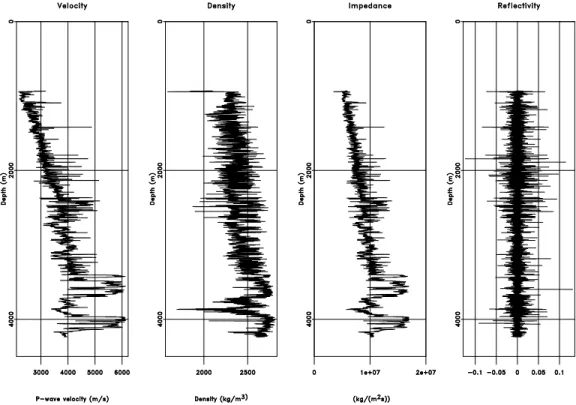
s(t) =r(t)∗w(t). (2.1) To estimate the earth’s reflectivity series as a function of time, one starts with the acoustic impedance as a function of depth,I(z), which is the product of compressional velocity, v(z), and density, ρ(z):
I(z) = v(z)ρ(z). (2.2) The seismic source is sensitive to changes in impedance, or reflectivity; mathemati-cally, the normal reflectivity is the difference in acoustic impedances divided by the sum of acoustic impedances between two layers (White and Simm, 2003).
r(z) = I(z+ ∆z)−I(z)
I(z+ ∆z) +I(z). (2.3) The estimation of reflectivity in depth from well log data is shown in Figure 2.1 using data from Penobscot L-30 well offshore Nova Scotia, Canada (Bianco, 2014). Interpolating Equation 2.3 from depth to time requires a time-to-depth relationship (TDR). There are several ways to compute a TDR. Using available checkshot surveys or vertical seismic profiles (VSP) can provide accurate measurements of seismic travel times to known depths; however, these surveys are not always available (White and Simm, 2003). An alternative approach is integrating the sonic log transit times:
T(z) = 2 Z z
zmin dξ
v(ξ), (2.4)
whereT(z) is the TDR are each depth,zmin is the minimum depth at which acoustic
used to effectively interpolate the reflectivity series to time:
r(t) =r(T(z)). (2.5)
The reflectivity series in time is then filtered with a seismic source to generate a synthetic seismogram as discussed in Equation 2.1. Using the velocity profile shown in Figure 2.1, I estimate a TDR to interpolate reflectivity from depth to time. The resulting reflectivity profile is convolved with a 25Hz Ricker wavelet to generate a synthetic seismiogram in Figure 2.2.
The one-dimensional convolutional model assumes normal incidence. In cases where this assumption reduces the quality of a seismic-well tie, there are several al-ternative approaches. One option is the Zoeprittz Equation or an approximation of the Zoeppritz Equation which generate reflectivity as a function of angle of incidence (Aki and Richards, 2002; Shuey, 1985). In cases where internal multiples and mode conversions must be considered another option is to model the reflectivity elastically. Mu˜noz and Hale (2015) use the propagator matrix method for vertically propagating plane waves in stratified media to model these complex effects (Kennett, 1986). Each method assumes stratified media and may provide a reflectivity series that is more representative of the earth’s reflectivity series as compared to one-dimensional con-volution. For the purposes of this thesis, I use simple one-dimensional convolution to estimate all synthetic seismograms.
Using the synthetic seismogram, I compare the modeled waveforms to real seismic data in Figure 2.3. This comparison helps the interpreter to understand how well log data and interpreted well facies relate to the seismic data. Using this understanding, it is possible to use the seismic data to gain a 3D understanding of structural, stratigraphic and potentially rock property distributions of the subsurface.
Bianco (2014) observes that to align the synthetic seismogram and real seismic data in Figure 2.3, a bulk shift can be applied to align the waveforms in the synthetic seismogram with the seismic data.
Figure 2.1: Example estimating impedance and reflectivity from well log data. The velocity and density data are from the Penobscot L-30 well offshore Nova Scotia, Canada. ch02-review/smpltie logs
The progression illustrated in Figures 2.1, 2.2, and 2.3 represents an idealized scenario where the velocity well log, density well log and seismic data are available. The well logs contain no missing section, and the forward modeled waveforms are consistent with real seismic data. In many cases, missing sonic or density logs can make it challenging or impossible to generate a reflectivity series that is representative of the well log data. A missing sonic log proves to be a significant challenge as it is crucial for generating a TDR. Furthermore, inaccuracies in seismic migration models
Figure 2.2: Example estimating a time-to-depth relationship using a well log velocity profile. Reflectivity in depth is interpolated to time using the time-to-depth relation-ship and convolved with a 25Hz Ricker wavelet to generate a synthetic seismogram. The velocity and density data are from the Penobscot L-30 well offshore Nova Scotia, Canada. ch02-review/smpltie logst
Figure 2.3: Synthetic seismogram modeled from well log data overlaying seis-mic amplitude data. The velocity and density data are from the Penobscot L-30 well and seismic data are from a dataset offshore Nova Scotia, Canada.
will cause a mistie between the waveforms modeled in a synthetic seismogram and real seismic data (White et al., 1998b).
Missing well log data prediction methods
Several approaches have been proposed to predict missing well log data. I will focus, in particular, on methods pertaining to predicting missing sonic and density logs as these logs are vital for modeling a synthetic seismogram and a seismic-well tie. A simple linear interpolation of missing log data between wells allows for estimation of a reflectivity series and TDR; however, this method does not account for variations in lithology or structure, so applying a TDR generated at one well to a nearby well may result in a mis-tie with the seismic data. In Figure 2.4, I remove a 1500ft interval of sonic log from the previous example. The resulting reflectivity series and modeled synthetic seismogram has a gap due to the missing sonic log, which may make it challenging to relate to the available seismic data.
Alternatively, several approaches are based on empirically derived relationships between one well log type and a different well log type. Gardner’s Equation has been shown to provide a reasonable relationship between sonic and density well logs data for a large number of brine saturated rock types (Gardner et al., 1974).
where
vp = P-wave velocity in f t
s ρb = Bulk density from log in
g cm3
α = Constant ≈ 0.23
β = Constant ≈0.25
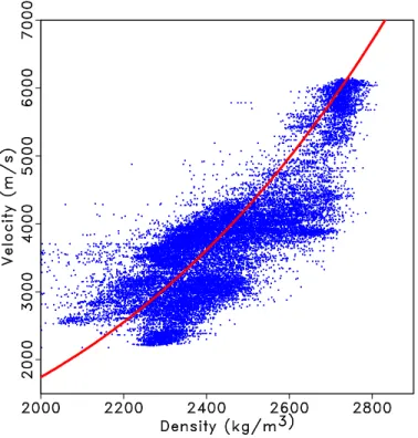
Using the previous example, I crossplot the available density and velocity data as well as Equation 2.6 in Figure 2.5. Gardner’s equation is a reasonable representa-tion of the available log data; however, the parameters α and β should be estimated for each stratigraphic interval; I will return to this understanding in chapter 3, where I propose to estimate missing well log data in the relative geologic time domain using Bayes’ Theorem. Using Equations 2.6, I estimate the missing section of sonic log shown in Figure 2.4 from the available density log. Results of this process are shown in Figure 2.6. The resulting synthetic seismogram may be a better representation of the subsurface at that location and does not have a gap due to missing information. Additionally, in wells where a resistivity log is acquired, the Faust method and Smith method provide empirical relationships between resistivity and sonic well logs (Faust, 1953; Smith, 2007). Alternatively, if there is a high interdependence of different well log types but the relationship is not inherently clear, Saggaf and Nebrija (2003) apply regularized back-propagation neural networks to estimate missing por-tions of sonic logs. Each empirical relapor-tionship may provide a useful approximation to a missing log; however, each method assumes that required logs are collected at every well location to carry out the estimation.
signifi-Figure 2.4: Example using linear interpolation to fill in the missing sonic log data. Using the resulting sonic log, a synthetic seismogram can be modeled; however, a gap is present due to the missing sonic log, which may make it challenging to relate to the available seismic data. ch02-review/smpltie logstmi
Figure 2.5: Crossplot of velocity and density log data from the Penobscot L-30 well. Using Gardner’s Equation, I relate the available sonic and density log data assuming
Figure 2.6: Example using Gardner’s Equation to fill in the missing sonic log data. Using the resulting sonic log, a synthetic seismogram can be modeled that might be a better representation of the subsurface at that location and does not have a gap due to missing information. ch02-review/smpltie logstgard
cantly in lateral space, which allows density and sonic logs from a nearby well to be used to estimate a TDR. This assumption does not take into consideration structural or stratigraphic variations in lithology. To account for these variations, the well must be correlated to a constant geologic time, which is analogous to stratigraphic cor-relation. Wheeler and Hale (2014) and Wu et al. (2017) use dynamic time warping (DTW) (Berndt and Clifford, 1994; Hale, 2013) to correlate multiple well logs. Shi et al. (2017b) use local similarity scan (LSIM) (Fomel, 2007a) to optimally sort and flatten multiple well logs. This well log correlation is analogous to a stratigrahpic correlation and may be convenient for stratigraphically constrained operations such as normalization. I will return to this observation in Chapter 3, where I propose to estimate missing well log data in the relative geologic time domain.
Automatic seismic-well ties
The manual seismic well tie involves matching common reflectors between modeled synthetic and seismic data by stretching and squeezing the synthetic un-til a desired correlation between the datasets is achieved (White and Simm, 2003). This procedure is a subjective, labor-intensive workflow that strongly depends on the interpreter’s experience and intuition. To reduce the interpreter bias and improve consistency among multiple seismic well ties, several automatic methods have been proposed. Mu˜noz and Hale (2012) use DTW to automatically align real and syn-thetic seismograms; this approach is extended to automatically and simultaneously tie multiple wells to seismic data by estimating a synthetic image to tie with the seismic image ensuring lateral consistency of the well ties (Mu˜noz and Hale, 2015). Further, Wu and Caumon (2017) show that laterally consistent seismic well ties are achieved by using DTW to correlate synthetic and seismic data that are ‘flattened’
to constant relative geologic time. An alternative approach to carry out the seismic well tie is LSIM; Herrera et al. (2014) compare DTW with LSIM, showing that both methods can successfully compute a seismic well tie. Their study shows that using DTW can achieve a higher correlation between synthetic and seismic data compared to LSIM; however, the resulting TDR using DTW shows an oscillatory behavior due to stretching and squeezing.
Interpolation along seismic structure
Once each well is tied to the seismic data, the high spatial coverage of seismic data can be utilized to understand lateral variations in log properties and check the consistency of seismic-well ties. Mu˜noz and Hale (2015) show that when wells are improperly tied to seismic data, there can be a qualitative mis-match in a well log interpolated cross section between wells. Several methods have been proposed to interpolate log data along local seismic structures. Assuming available log data is properly tied to a nearby seismic trace and conforms to seismic image features, Hale (2010) uses image-guided blended-neighbor interpolation (Hale, 2009) for seismically guided well log interpolation. Alternatively, Karimi et al. (2017) show that predictive painting (Fomel, 2010) can be used to interpolate log data along seismic structures to generate accurate starting models for post stack inversion. Fomel (2016) presents a fast interpolation algorithm for interpolating scattered data to a regularly sampled grid. Interpolation along seismic structure using well log data generates log property volumes that conform to both well log and seismic datasets. Wu (2017) proposes to compute such a structurally conformable model in the flattened space, where the seismic data is first unfaulted and unfolded, then well log data are interpolated in the flattened domain. After interpolating the well log data, the model is returned to the
original domain.
In this thesis, I adopt predictive painting to interpolate well log data along seis-mic structure. Predictive painting is defined using plane-wave destruction filters that measure the local slopes of seismic events (Fomel, 2002). The plane-wave destruction operator can be written in linear operator notation
r =Ds (2.7)
where s is a group of seismic traces from a seismic image (s= [s1s2...sN]T), r is the
destruction residual, and D, the destruction operator, is defined as
D = I 0 0 . . . 0 −P1,2 I 0 . . . 0 0 −P2,3 I . . . 0 .. . ... ... . . . ... 0 0 . . . −PN−1,N I (2.8)
whereI is the identity operator andPi,j describes the prediction of tracejfrom trace
iby shifting along the local slope of the seismic data. Slopes can be estimated in this way by minimizing the prediction residual operator r using regularized least-squares optimization. The prediction of one trace from another trace (Fomel, 2010) can be defined as
sk =Pr,ksr (2.9)
where sk is the unknown trace and sr is the reference trace. The predictive painting
operator is defined as:
P1,k =Pk−1,k. . . P2,3P1,2 (2.10)
Predictive painting spreads information along local seismic structures to generate volumes of well log data from a single well log reference trace providing a method to predict an expected log profile in a location with no well log data.
Additionally, Karimi et al. (2017) show that several well logs can be combined by weighting the interpolation based on the lateral distance from the reference well as defined by a radial basis function (RBF) (Powell, 1985). The RBF has a higher weight for distances closer to the well location as compared to farther away. The RBF can be combined with interpolated log property volumes generated from data at each well location using the following interpolant:
V(x) = PN k φ(|x−xk|)Sk(x) PN k φ(|x−xk|) (2.11) where Sk is the volume created by spreading log data from locationxk to the entire
seismic data set using predictive painting weighted by the RBF, φ(m), andN is the total number of wells used in the interpolation. Recently, Shi et al. (2017a), propose an approach that combines the RBF with the distance along seismic structure to weight the interpolation providing a more intuitive weighting scheme as compared to weighting based only on lateral distance from the well.
LOCAL SIMILARITY METHOD*
The workhorse behind many of the proposed methods in this thesis is the local similarity method (LSIM), which is a data matching technique. Matching datasets involves aligning similar waveforms between two datasets. Whether aligning two logs from different wells or aligning a modeled synthetic seismogram with a seismic trace, I focus on matching a response that corresponds to similar lithologies between the two datasets or a constant geologic time. In comparing two datasets, the purpose is to estimate a smoothly varying warping function, Sk, required to align one dataset,
hk, to a reference dataset, rk,
rk(t)≈ hk(Sk(t)) (2.12)
I can represent the warping function with the shifts, gk(t), as follows:
Sk(t) = t+gk(t) (2.13)
where the t denotes the original independent axis and gk(t) are the shifts required
to match the datasets as defined in Equation 2.12. The correlation coefficient can be used to quantify the quality of the match between datasets (Hampson-Russell, 1999). The LSIM method begins with the observation that the correlation coefficient (c) only provides one number to describe the datasets; however, I am interested in understanding the local changes in the datasets’ similarity. Therefore, the LSIM method computes local similarity ct, which is a function of time, t. The square of c
can be split into a product of two factors (Fomel, 2007a):
c2t = rt ∗ht (2.14)
wherert andht are the solutions to the following regularized least-squares problems,
respectively min rt (X t (at −rtbt)2 +R[rt]) min ht (X t (bt −htat)2+R[ht])
The regularization operator,R, is implemented using shaping regularization (Fomel, 2007b) and designed to enforce smoothness. To estimate the solution, LSIM is cal-culated for a series of shifts. The results of this calculation are accumulated and displayed on a ‘similarity scan’ as shown in Figures 2.9 and 2.11 in the following
synthetic example. From the similarity scan, I select the series of shifts along the entire length of the reference dataset that optimally aligns the two datasets (Fomel and Jin, 2009).
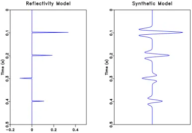
To illustrate the alignment of two datasets using local similarity, I use two examples based on the simple model shown in Figure 2.7. In our first example, I apply a 40ms shift to the modeled synthetic seismogram and use LSIM to estimate the shifts to realign the shifted synthetic model with the original synthetic model (Figure 2.8). Estimation of the shifts for the first example is visualized in a local similarity scan shown in Figure 2.9. In our second example, I add 15% random noise to the reflectivity model and convolve the noisy reflectivity with a 30Hz Ricker wavelet to create a noisy reference trace. LSIM is used to estimate the shifts to realign the shifted synthetic model with the noisy reference trace in Figure 2.10. Estimation of the shifts for the second example is visualized in a local similarity scan shown in Figure 2.11. From our synthetic examples, I observe that shifts can be accurately estimated to align a modeled seismogram with both a noise-free and noisy reference seismograms.
Figure 2.7: Reflectivity series in time (left) convolved with a 30Hz Ricker wavelet to model a seismogram (right). ch02-review/synthetic-example modelb
Figure 2.8: Modeled seismogram (left), modeled seismogram shifted by 40ms (mid-dle), re-aligned seismogram using the shifts estimated from the local similarity scan (right). ch02-review/synthetic-example shifted-matched
Figure 2.9: Similarity scan and picked optimal shifts (white curve). Warm colors represent high similarity whereas cool colors represent low similarity.
ch02-review/synthetic-example scanch2
Figure 2.10: Noisy reference trace (left), modeled seismogram shifted by 40ms (mid-dle), re-aligned seismogram using the shifts estimated from the local similarity scan (right). ch02-review/synthetic-example noise-matched
Figure 2.11: Similarity scan and picked optimal shifts (white curve). Warm colors represent high similarity whereas cool colors represent low similarity.
ch02-review/synthetic-example scan-noise
WELL LOGS AND VELOCITY MODEL BUILDING
Mis-ties between the modeled synthetic seismograms and seismic data can be used to update the well’s TDR and explained by inaccuracies in either the seismic phase or seismic migration velocities (White et al., 1998b; Henry, 2000). I will fo-cus on the relationship between inaccuracies in the seismic migration model and the resulting seismic well tie mis-tie. In an attempt to reduce the mis-tie between well log information, which is taken as the ground truth, and the seismic image, well log measurements can be injected into migration velocity model building to provide constraints in an otherwise non-unique problem (Bakulin et al., 2010). Morice et al. (2004) show that combining well log, borehole and surface seismic data can provide an understanding of seismic velocities, anisotropy, attenuation and interbed multi-ples, and can further aid in building a velocity model consistent between all datasets.
Egozi et al. (2006) show that mis-tie surfaces generated from multiple picks in mul-tiple wells can be used to iteratively update a TTI velocity field thus driving the cumulative average mistie of all wells towards zero. Using well marker-related work-flows in velocity model building removes or reduces non-uniquness and may allow for simultaneous estimation of velocity and anisotropy parameters which can be used to constrain tomography problems that focus on flattening the residual moveout of seismic events (Woodward et al., 2008; Bakulin et al., 2010). Although, well marker-related workflows help integrate well log interpretations with seismic velocity model building; these methods are limited to updates related to only discrete pre-selected well markers.
The literature referenced above is by no means exhaustive; however, the work-flow for including ‘well data’ is consistently based on the tomography principle us-ing the depth mismatch between tops selected in logs and depth seismic interpre-tations. Beyond short discussions by White et al. (1998b) and the relationship be-tween the mis-tie and velocity well log update (Mu˜noz and Hale, 2015; Herrera et al., 2014), there is little discussion in the literature about the interpretation of mis-ties in isotropic and anisotropic media. This general lack of understanding clouds the relationship between well log velocity, migration velocity, synthetic seismograms and seismic data, which should ideally be interpreted in a consistent way.
Chapter 3
Missing Log Data Estimation
In plays where the number of wells drilled outnumbers the number of sonic and density logs acquired, estimating missing logs is an essential step to understand how changes observed in well logs relate to amplitude variations in seismic data. I estimate a complete sonic log using all other sonic logs in the dataset and compare it against the actual sonic log from the well. These results are also compared against Reverse Gardner’s equation for estimating missing sonic logs. I then extend the approach to honor true well log values for well logs that have incomplete or partial well logs.
There are several potential sources of information that can be used to constrain the estimation of missing log data: (1) the same well log type at other well locations, (2) other well logs within the same well, and (3) the seismic data. In the first section, I focus on using other well logs of the same type type in our estimation of a missing log. In the second section, I extend the approach to include models that relate different well log types and uncertainty to estimate a missing log using Bayes’ Theorem.
Missing log data interpolation*
In this section, I focus on using other well logs of the same type in our esti-mation of a missing log. Generally, we include inforesti-mation from all other wells in our estimation: W1 W2 .. . WN ˜ l ≈ W1lˆ1 W2lˆ2 .. . WNlˆN (3.1)
where our estimated log, ˜l, is a weighted function of well logs from different wells denoted by the subscript k. If I simplify the prediction to one unknown log and one known log, Equation 3.1 simplifies to the following linear relationship:
Wk(z)˜l(z) ≈Wk(z)lk(Sk(z)), (3.2)
where Wk(z) weights the specific value used to estimate the missing log value,˜l(z),
from an available well logs, lk(Sk(z)). To estimate a missing log at each depth
sample, I must remove structural and stratagraphic variations between the well logs by correlating the well logs to common geologic time using function, Sk(z), based on
the shifts estimated from LSIM. The correlation is done by selecting a well log type that is available in all wells, for example, gamma ray. We, then, select one reference gamma ray log and estimate the function, Sk(z), that aligns all remaining gamma
ray logs to the reference. Sk(z)is applied to the remaining well logs to align all well
logs (e.g., density and velocity) to constant geologic time.
I design the weight,Wk(z), in Equation 3.2, as a product of two factors: the
distance between the unknown and available well logs and the caliper value at that depth, which measures the size of the borehole at each depth. I make the assumption
that deviations in the caliper from the anticipated borehole size while drilling likely indicates an inaccurate log measurement. Thus, Wk(z)can be expressed as:
Wk(z) = φ(|x−xk|)∗Ck(Sk(z)), (3.3)
whereφ(|x−xk|)is a radial basis function,xk is the well location,xis the well with
a missing log, and Ck is inversely proportional to the deviation between the expected
and actual caliper value at each depth.
There are several different radial basis functions, and I chose to implement the inverse multiquadratic radial function
φ(|x−xk|) =
1 p
1 + (|x−xk|)2
, where > 0 (3.4) which gives a larger weight to a well closer to the unknown well as compared to a well farther away.
Returning to our original linear relationship, Equation 3.1, the estimated log, ˜
l, is a function of available well logs and weighted by each well’s distance and caliper log. By solving the least-squares problem in Equation 3.1, I can predict a new ‘pseudo well log’ at each depth as follows:
˜ l(z) = N P k=1 Wk2(z)lk(Sk(z)) N P k=1 W2 k(z) (3.5)
I use wells from the Teapot Dome dataset from Wyoming made available by the U.S. Department of Energy and RMOTC to test the proposed approach. Over 1000 wells have been drilled into the anticline structure. I select a limited subset of the 26 longest wells for our examples summarized in Table 3.1. Several wells have
missing sonic or density logs making it challenging to integrate the available log and seismic data. In this section, I focus on using the sonic, density, caliper and gamma ray logs to estimate a complete sonic and density well log suite that are the minimum required logs to estimate a TDR and model a synthetic seismogram to perform a seismic well tie. Table 3.2 summarizes the initial well log dataset that is used in this section.
Table 3.1: Well logs used in examples. Data pulled directly from Teapot Dome dataset made available by the U.S. Department of Energy and RMOTC.
UWI Sonic Density NPHI Caliper1 Caliper2 Gamma Ray1 Gamma Ray2
49025109020000 X X X 49025107090000 X X X X X 49025109200000 X X X X X 49025110490000 X X X X 49025106100000 X X X X X 49025110120000 X X X X 49025107450000 X X X X 49025108070000 X X X X 49025110700000 X X X 49025107690000 X X X X 49025107260000 X X X X 49025107290000 X X X X 49025109720000 X X X X 49025109370000 X X X X X 49025102650000 X X X X 49025108310000 X X X X X 49025109650000 X X X X X 49025109730000 X X X X X 49025109660000 X X X X X 49025105980000 X X X X 49025109060000 X X X X X 49025109710000 X X X X 49025106090000 X X X X 49025108910000 X X X X 49025108970000 X X X X 49025102700000 X X X
Derived from1resistivity and2density logs
Table 3.2: Well log data statistics for sonic, density, caliper and gamma logs Log Type Wells Sonic Density Caliper* Gamma*
Number 26 15 22 26 26
Mean Length (ft) 4192 2646 3093 4074 4074
*Derived from resistivity and density logs as provided with the dataset made available by RMOTC.
the warping function, Sk(z). Because a form of a gamma ray log are available in all
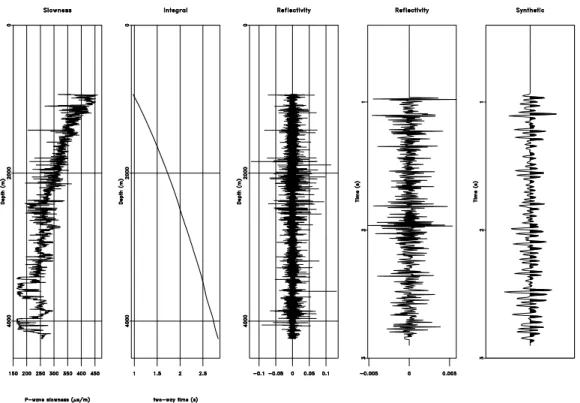
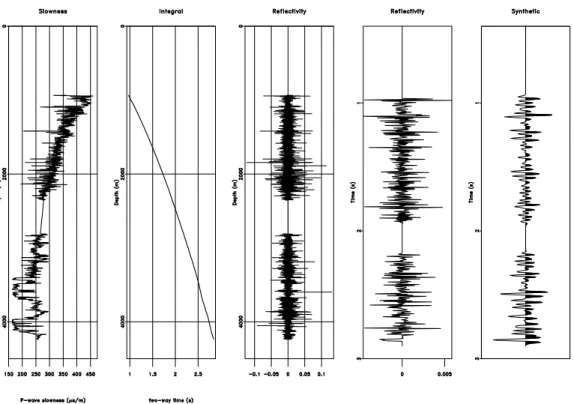
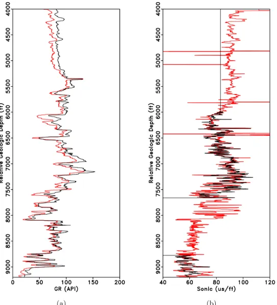
wells, I use the gamma logs to estimate the warping function. The longest gamma ray log is selected as the reference log, r(z). The shifts are estimated by matching the gamma ray log from each well to the reference gamma log as shown in Figure 3.2(a). The alignment shifts are then applied to the remaining well logs at each well to align all well logs to constant geologic time. Results of aligning a sonic log before and after applying the shifts estimated from aligning the gamma ray logs are shown in Figures 3.1(b) and 3.2(b), respectively.
This approach results in a well log dataset flattened along constant geologic time. The log data might be collected over several years, with different logging tools, and likely different techniques applied to process the data. To account for this variability, I normalize the sonic and density logs using the big histogram method (Shier et al., 2004). For normalization, I select 15 intervals based on available well log tops and lithology variations. I estimate the cumulative mean and standard deviation for all well log data in each interval. I assume that the distribution of well log data from each well, in each interval, should fall one standard deviation of the cumulative mean. Normalization in the constant geologic time domain requires little interpreter input as each log is inherently stratigraphically correlated. With the aligned and normalized sonic logs, I estimate the missing sonic logs, or sections of sonic logs using Equation 3.5.
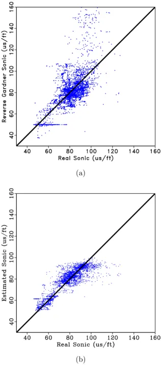
I perform a blind well test to validate the proposed approach by estimating a sonic log in a well where a real sonic log is available; the estimated sonic log is crossplotted against the real sonic log for the entire well in Figure 3.3(b). For comparison purposes, I use available density information and the Reverse Gardner Equation (Gardner et al., 1974) to estimate a sonic log; this result is crossplotted
(a) (b)
Figure 3.1: (a) Median filtered gamma log from the reference well (red) and median filtered gamma log from a second well (black). (b) Sonic log from the reference well (red) and sonic log from a second well (black).
(a) (b)
Figure 3.2: (a) Median filtered gamma log from the reference well (red) and an aligned gamma log from a second well (black) after applying estimated alignment shifts. (b) Sonic log from the reference well (red) and an aligned sonic log from a second well (black) after applying estimated alignment shifts from matching gamma logs. ch03-logs/../interpPaper/logs GR2shift0,DT2shift0
against the real sonic log for the entire well in Figure 3.3(a). When estimating the Reverse Gardner Equation, I break the well into 15 intervals based on well tops and changes in lithology from the gamma ray log, and I recompute the equation that best fits the data for each interval. I observe significant improvement of the proposed approach over a conventional method for estimating a missing sonic log. Results comparing the sonic log estimated using the proposed approach against the real sonic log along two 1600 ft intervals are shown in Figure 3.4.
(a)
(b)
Figure 3.3: (a) Real sonic log cross plotted against the sonic log es-timated using Reverse Gardner equation. (b) Real sonic log cross plotted against the sonic log estimated using the proposed approach.
(a) (b)
Figure 3.4: I perform a blind well test by estimating a sonic log using the proposed approach and comparing the result against the real sonic log. Real sonic log (black) versus estimated sonic log (blue) along two 1600ft intervals along the reference log.
From Equation 3.4, there are two user selected constants: in the RBF and the weighting of the caliper, Ck. To select optimal values for these constants, I minimize
the average RMS error of every predicted sonic and density log against the actual sonic and density logs.
RM Serror = N P k=1 zmax P z=0 q ( ˜lk(Sk(z))−lk(Sk(z))2 N (3.6)
where l˜k is the blind well test prediction of log k and lk is the actual log k. This
minimization problem is visualized in Figure 3.5 where Equation 3.6 is solved for different values of in Equation 3.4 when estimating a sonic and density log.
(a) (b)
Figure 3.5: (a) RMS error between real and predicted sonic logs given all wells in the dataset and values. (b) RMS error between real and predicted density logs given all wells in the dataset and values. ch03-logs/sens epsdt,epsrhob
I normalize and combine the results shown in Figures 3.5 to select a single value of that minimizes Equation 3.6 for sonic velocity and density. The constant controlling the weighting of the caliper, Ck, is also estimated by combining the
combination are shown in Figure 3.6, where I observe minimum normalized RMS error when = 0.0001 and weightcaliper = 0.423.
(a) (b)
Figure 3.6: (a) Normalized combined sonic and density RMS error given all wells in the dataset and values. (b) Normalized combined sonic and density RMS error given all wells in the dataset and caliper weighting values. ch03-logs/sens eps,cal
From Table 3.2, I observe that most wells have a sonic and density log; however, the difference between the mean length of the sonic/density logs as compared to the gamma log indicates that several of the well logs were not acquired over specific intervals or have missing sections as shown in Figure 3.2(b). For well logs that have missing sections, I include the available log data in Equation 3.5 to honor the available measurements and interpolate the missing log sections. In Figure 3.7 we interpolate missing log data where there are holes in the original log and make use true well log measurements when available.
The proposed approach is applied to 26 wells from the Teapot Dome dataset to generate complete sonic and density logs for each well. Table 3.3 summarizes the log dataset after estimating missing or incomplete logs.
(a) (b) (c)
Figure 3.7: (a) Original sonic log (black) versus estimated sonic log (blue). (b) Original density log (black) versus estimated density log (blue). The original well log data is used in the inversion so areas where sonic or density data is available the estimated logs match the original data. In the interval between 3500 ft and 3900 ft, there is a significant deviation in the (c) caliper log indicating an inaccurate measurement; therefore, the estimated log deviates significantly from the original log.
Table 3.3: Well log data statistics after estimating sonic and density logs for all wells Log Type Wells Sonic Density Caliper* Gamma*
Number 26 26 26 26 26
Mean Length (ft) 4192 3991 3639 4074 4074
*Derived from resistivity and density logs as provided with the dataset made available by RMOTC.
number of logs and length of the logs available to integrate with the available seismic data. Using the interpolated sonic and density logs, it is possible to compute a TDR and reflectivity series to tie any given well to seismic data. The proposed method addresses several challenges in integrated studies, specifically interpolating missing well logs at wells that have incomplete well log suites and may be a useful data integration tool in onshore plays where the number of wells drilled is much higher compared to the number of sonic and density log acquired.
Although this method addresses several challenges, I focus on interpolation techniques that assume that rock-properties do not vary significantly laterally and make several additional assumptions related to the interpolation of missing log data:
1. Gamma logs are matched to estimate the alignment shifts; therefore, estimated section is limited to a section in each well with an available gamma log.
2. All gamma logs are aligned with a single reference gamma log and the esti-mated log section is limited to the stratigraphy found in this reference log. This reference well log can be thought of as a type log which contains the entire stratigraphic column observed in other well logs.
3. I did not perform fluid substitution prior to solving equation 3.5 for each well. The proposed approach is based on interpolation, and I assume fluid substitu-tion to have a negligible impact on the results. This assumpsubstitu-tion may present
challenges in reservoirs where hydrocarbons impact the well response within the same stratigraphic interval.
These assumptions may not be valid in geologically complex areas with significant stratigraphic variations such as unconformities or channels where entire stratigraphic units may be absent due to erosion. Additionally, the well log correlation approach, may meet similar challenges as those experienced by conventional, interpreter driven, workflows where rapid stratigraphic variability (e.g. slope deposits, clinoforms, etc.) may not correlate, or may correlate ambiguously in several places, between wells. Although I did not account for changes in the fluid content, the proposed approach provides a reasonable first-order approximation of the unknown well logs. The pre-dicted velocity and density well logs provides the minimum required logs to forward model a synthetic seismogram and tie the well with real seismic data, which is dis-cussed in the next chapter.
Missing well log data prediction using Bayes’ theorem*
The previously proposed method for missing log data prediction is useful; how-ever, the method is based on interpolation and does not consider information at the same well location. Additionally, well log data do not perfectly conform to empirical estimations (see Figure 2.5); there is often scatter of the real data around the em-pirical models. Methods that consider all well log data and the uncertainty of these measurements relative to empirical estimations and models might provide the best approach to estimating missing log data. Avseth et al. (2010) show that probabilisti-cally modeling reflectivity from distributions ofVp,Vs, andρand comparing modeled
gradient-intercept against inverted gradient-intercept data from seismic amplitudes results in a facies distribution consistent with observations from wells. I theorize that using a distribution around a model will improve on the previously proposed method of missing well log prediction.
I propose a method to estimate missing sonic logs in the relative geologic time domain using sonic logs acquired at other wells as well as non-sonic well logs at the well with the missing sonic log. I first correlate a reference gamma log from each well using LSIM and employ the estimated shifts to align all available logs. In the relative geologic time (RGT) domain, I interpolate a missing sonic log according to the previously proposed approach, using sonic logs acquired at other wells; this result is treated as a priori information. I then use the stratigraphically correlated sonic, density and neutron porosity logs to perturb the a piori information using Bayes’ theorem. The maximum a posteriori estimate is compared against the actual sonic log using a blind well test. Results of this method show an improvement over previously proposed methods that use only one of the three available sources of information to predict a missing well log.
I perturb the interpolated sonic log from Equation 3.5 based on available density and neutron porosity logs acquired at the well of interest. If I treat the inter-polated sonic result as prior information, p(m), I use Bayes’ theorem to estimate a posterior result given a likelihood function based on porosity and density logs acquired at the well of interest, l(d|m), as follows:
σ(m|d) ∝ l(d|m)p(m) (3.7) The likelihood function incorporates correlated modeled distributions between
sonic, density and porosity based on the well log data in each stratigraphic interval. The trends for the correlated distributions are from empirical relationships: Gardner’s relationship, which relates sonic and density log data for a large number of brine satu-rated rocks, and the general relationship between bulk density and porosity (Gardner et al., 1974). I start with Gardner’s relationship to relate density to velocity,
ρb =αvβp. (3.8)
where
vp =P-wave velocity in ft/s
ρb =Bulk density from log in g/cm3
α=Constant, estimated for each stratigraphic interval β =Constant, estimated for each stratigraphic interval
I combine Gardner’s relationship with the general relationship between bulk density and porosity,
φT = ρm −ρb ρm −ρf , (3.9) where ρm =Matrix density in g/cm3 ρf =Fluid density in g/cm3
to obtain a relationship between p-wave velocity and total porosity, φT =
ρm−αvβp
ρm −ρf