Procedia Computer Science 60 ( 2015 ) 1070 – 1080
1877-0509 © 2015 The Authors. Published by Elsevier B.V. This is an open access article under the CC BY-NC-ND license (http://creativecommons.org/licenses/by-nc-nd/4.0/).
Peer-review under responsibility of KES International doi: 10.1016/j.procs.2015.08.152
ScienceDirect
19th International Conference on Knowledge Based and Intelligent Information and Engineering
Systems
GPU-PSO : Parallel Particle Swarm Optimization approaches on
Graphical Processing Unit for Constraint Reasoning: Case of
Max-CSPs
Narjess DALI
a, Sadok BOUAMAMA
aaCOSMOS Laboratory,National School of Computer Science,University of manouba, Tunisia
Abstract
Constraint Satisfaction Problems (CSPs) occur now in different domains. Several methods are used to solve them. In particular, Particle Swarm Optimization (PSO) allows to solve efficiently CSPs by significantly reducing the calculation time to explore the search space of solutions. However, this metaheuristic is excessively costing when facing large instances.
In this paper we address the Maximal Constraint Satisfaction Problems (Max-CSPs). We introduce a new resolution approach that allows solving efficiently the Max-CSPs even with large instances. Our purpose is to implement a PSO based method by using the GPU architecture as a parallel computing framework. In particular, we focus on the implementation of two parallel novel approaches. The first one is a parallel GPU-PSO for Max-CSPs (GPU-PSO) and the second one is a GPU distributed PSO for Max-CSPs (GPU-DPSO). Our experimental results show the efficiency of the two proposed approaches and their ability to exploit GPU architecture.
c
2015 The Authors. Published by Elsevier B.V. Peer-review under responsibility of KES International.
Keywords: particle swarm optimization; Maximal Constraint satisfaction problems; GPU- computing
1. Introduction
Real optimization problems are often complex and NP-hard. Besides, in terms of constraints and objectives, their modeling is continuously evolving and their resolution requires more and more CPU time. Even quasi-optimal algorithms, such as metaheuristics, becomes insufficient when it comes to solve large size problems. Among these problems we find the constraint satisfaction problems CSPs10.
CSPs are the focus of many artificial intelligence applications and operational researches, such as resources allocation, planning and scheduling... . A CSP P=(X,D,C) is defined as follows:
• Set ofnvariablesX={x1, ...,xn}.
• SetD={D1, ...,Dn}ofndomains :Diis the set of possible values that can takes the variablexi. ∗Corresponding author. E-mail address : [email protected]
© 2015 The Authors. Published by Elsevier B.V. This is an open access article under the CC BY-NC-ND license (http://creativecommons.org/licenses/by-nc-nd/4.0/).
• SetC ={C1, ...,Cm}ofmconstraints on an arbitrary subset of variables inX. A constraintCiis called n-ary when it is defined by a set ofnvariables:Ci={xi1, ...,xin}. By applying specific rules, n-ary constraints could be transformed into binary constraints10. The constraints can be defined in intension by functions or predicates, or in extension by a list of all valid combinations of values of variables that define the constraint.
Solving a CSP is finding a set of values corresponding to each variable so that all the constraints are satisfied. In other words, a CSP solution is a complete instantiation that satisfies all the constraints.
The CSP formalism enables a problem to be modeled as a fixed network with constraints that must be satisfied. Prac-tically, many existing problems are difficult to solve or have no solution that can satisfy all the constraints. In this case, it is best to find instantiation that satisfies as many constraints as possible. Such problems are called Maximal Constraint Satisfaction Problems Max-CSPs4.
Max-CSPs deal with complete or incomplete methods. Complete methods, based on backtrack principle like forward checking4, are able to provide optimal solutions. Unfortunately, they come with a major disadvantage which is the
combinatorial explosion. Incomplete methods, such as metaheuristics ( genetic algorithms2, particle swarm
optimiza-tion1, etc), aim to avoid the trap of local optima. Although these latter methods do not guarantee finding an optimal
global solution, they assure efficiency in terms of computation time and memory space.
Since the evolution of many-cores architecture, parallel programming fields has been evolving significantly, espe-cially over graphical processing units (GPUs) computing which is well-known for its powerful way to realize high performance parallel computing in some important scientific applications3. The evolution of graphical processors
has been contributing to the improvement of graphical cards. Their computing power has been rising significantly in non-graphical applications7. Like many other application fields, combinatory optimization over GPU represents a
significant interest. The aim of this work is to implement parallel PSO algorithms in order to get the maximum effi -ciency while solving large size Max-CSPs using GPU architecture. This paper aims to propose two GPU parallel PSO approaches for Max-CSPs and is organized as follows: The second section presents the overall context of our work. The third presents related work. The forth section describes the contribution of our work: our first proposed GPU-PSO approach (GPU-PSO) and our second proposed approach (GPU-DPSO). The fifth presents the experimental results of our proposed approaches. Finally, this work ends with a conclusion and possible extensions.
2. Overall context
2.1. GPU architecture
Although they are originally designed for graphical applications, GPUs witnessed a significant evolution over the last few years into a powerful many-core architecture with an increasing high performance computing performances for general applications. Nevertheless, to benefit from this high performance we need to build far more complex programs than what we did in the sequential programs3. Thus, unlike CPUs, GPUs are oriented to highly parallel
computing due to their conception that provide more transistors to compute and to manage the data flow.
2.1.1. NVIDIA GPU
Upon the arrival of the CUDA development kit of NVIDIA8, the use of GPU in various scientific and engineering
computing tasks has risen significantly.
The NVIDIA GPU architecture is built around a scalable array of multithreaded Streaming Multiprocessors (SMs)8.
When a CUDA program on the host CPU invokes a kernel grid, the blocks of the grid are enumerated and distributed on multiprocessors with available execution capacity. The threads of a thread block execute concurrently on one multiprocessor, and multiple thread blocks can execute concurrently on one multiprocessor. As thread blocks ter-minate, new blocks are launched on the vacated multiprocessors. A multiprocessor is designed to execute hundreds of threads concurrently. To manage such a large amount of threads, it employs a unique architecture called SIMT (Single-Instruction, Multiple-Thread)8.
2.1.2. Memory Hierarchy of NVIDIA GPU
Threads access the data located in several memories8. Every thread has a local memory. Blocks have a shared
memory accessible only by their own threads and allows them to synchronize and to communicate with each other. Blocks have also registers accessible by threads. Threads of different Blocks can only communicate via the global memory. There is also two read-only memories; the constant memory and the texture memory.
2.2. PSO algorithm
Particle swarm optimization (PSO) was invented, in 1995, by Russel Eberhart and James Kennedy5.
The PSO algorithm is a stochastic method. This method is inspired from the behavior of bird flocking, which principle is based on the individuals’ movement to explore the search space. Each individual of the swarm contribute with his experience to the evolution of the group and uses the global experience of the group for its own evolution. Thus, the information passes in both directions, from the group to the individual and from the individual to the group.
The algorithm starts with a random initial population called swarm. In each iteration, individuals are evaluated and the values of their objective function are compared. The individual having the best value of objective function, called Fitness, is considered as guide for the next iteration; the other particles of the population will join it. In addition to this component, each particle retains its previous best local position. Thus, particles will explore the most promising regions where optimal solution is more luckily to be found. The mathematical formulation chosen to define the movement of a particle in the search space is inspired by the version of PSO presented by Shi and Eberhart using the inertia weight model12. The advantage of this formulation is the use of coefficients which are independent from the problem to optimize. Each particle is characterized by three space variables vectors: its positionXi(t), its velocity
Vi(t) and its best local positionXPbesti(t) ( the position where the Fitness value found by the particle is maximal). The
components of these vectors are respectively defined by Equations (2) and (1).
vi j(t+1)=w∗vi j(t)+c1r1j(t)(xPbesti j(t)−xi j(t))+c2r2j(t)(xGbest j(t)−xi j(t)) (1)
xi j(t+1)=xi j(t)+vi j(t+1) (2) Wherevi j(t), xi j(t), xPbesti j(t) andxGbest j(t) are respectively the velocity, the current position, the best local position
and the best global position ( best position reached by a particle in the overall swarm) of particleiin dimension jat iterationt. j=1, ...,|Di|. The calculation of the new componentvi j(t) of the velocity vectorVi(t) of particleiincludes the jthcomponent of: its previous velocity value, its best local position and the best global position. Equation (1). A new componentxi j(t) of the position vectorXi(t) of particleiis updated by its previous position and its new velocity. Equation (2).
r1j(t) andr2j(t) are random values between 0 and 1. w,c1andc2are positive parameters and represent respectively
the inertia, the personal influence and the social influence. The PSO algorithm is presented in Algorithm 1.
Algorithm 1PSO Algorithm
Initialize the positions and velocities of all particles
repeat
for1toparticleNbr do
Compute Fitness value
Update best local positionXPbest i
Update best global positionXGbest i
Update VelocityVi(t+1) Update positionXi(t+1)
end for
3. Overall related work
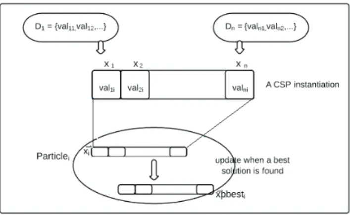
To solve a Max-CSP using PSO, we have to determine the search space of the swarm, the particles, their positions
and their velocities1. A position of one particle is a complete instantiation (val1,val2, ...,val
n) to the CSP variables
(x1,x2, ...,xn) respectively as shown in Figure 1. Particlei’s best positionXPbest iand the swarm’s best positionXgbest ,
are the best solutions so far found byParticleiand by the entire swarm respectively. The velocity of a particle is an
n-dimensional vector that moves the particle from its previous position.
Fig. 1. The particle position in the CSP status
3.1. The Dynamic Distributed Double Guided Particle Swarm Optimization for Max-CSPs(D3GPS O)
Many works focused on the resolution of CSPs using PSO. Among them we find The Dynamic Distributed Double
Guided Particle Swarm Optimization for Max-CSPs (D3GPS O)1. In nature, when looking for their food, birds are
gathered in several swarms. Each swarm occupies a zone in the same country, and the first to find a nourishment source will be followed by the others. This natural swarming theory presents an inspiration for science and consists in
dividing the search space into sub-spaces. Multi-agent approach is used for this purpose in1: each agent has in charge
the responsibility of one sub-space. A given sub-space consists of particles having the same Fitness value i.e particles that violate the same number of constraints.
Global dynamic ofD3GPS O: For a given CSP, an agent referred to as interface agent, randomly generates an initial
swarm. This swarm is split into sub-swarms according to their specificities i.e. the fitness value range FVR: each sub-swarm hold in particles having their Fitness value in the same range FVR. For each sub-swarm, an agent called
Species agent,S peciesFVR, is created. EachS peciesFVRruns its own PSO algorithm on its sub-swarm and calculates
the number of constraints violated NCV for each particle. If this number is equal to FVR of the Species agent that
the particle belongs to, then this particle remains in thisS peciesFVR. Else, two types of processing are possible: the
particle will be sent to the group of particles having its same Fitness value, or it will be sent back to the interface agent if no Species agent matches its Fitness value, where a new one is created, assigned NCV as specificity (Fitness value) and containing the particle in question. Afterward, the interface agent informs the other Species agents about the recently created one. Then this latter begins the PSO process. The agents will repeat this processing as long as the stopping condition is not reached.
For this approach, the stopping condition is the number of generations that any agent shall not exceed. If aS peciesi
meets a particle that satisfies all the constraints before reaching the last iteration, it sends that particle to the interface agent, which informs all Species agents to stop their PSO process. Otherwise, at the last iteration, they successively transmit, among their particles, a randomly chosen one. Each of these particles has a Fitness value equal to the FVR of its corresponding Species agent. The interface agent picks the best of these particles (which violates the minimum constraints).
3.2. GPU-based Parallel Particle Swarm Optimization
Recently, many researches done on the optimization field have used GPU to implement metaheuristics. For in-stance, in6 the authors present the implementation of the island model for evolutionary algorithms on GPU. The
results of their work showed that GPU computing allows to speed up significantly the search process. You Zhou and Ying Tan13proposed a novel parallel approach to run standard particle swarm optimization (SPSO) on Graphic
Pro-cessing Unit (GPU). In their approach, the block size and the grid size are setting with a number of threads equaling to N which is the total number of particles. The N threads do exactly the same operation simultaneously and syn-chronously. The test performance of this approach was based on four classical benchmark test functions. Based on the experimental results of You Zhou and Ying Tan13,we can deduce that GPU can accelerate the computing speed
greatly.
4. Contribution
4.1. Our first approach : GPU-PSO algorithm for Max-CSPs (GPU-PSO)
PSO structure is almost intrinsically parallel which enable its efficient implementation using parallel computing architecture. For further efficiency, PSO algorithm is totally parallelized on GPU to minimize data transfer between host memory and the global GPU memory.
Our GPU-PSO consists in the implementation of PSO algorithm for Max-CSPs described previously in parallel man-ner while maximizing the use of the graphical processing unit.
The algorithm starts with a random initial swarm. Then, particles will seek their Fitness by executing the objective function. Since calculating the Fitness, the position and the velocity of one particle is independent from the other particles, these tasks will be executed in parallel on the GPU6,13.
4.1.1. Cuda implementation of GPU-PSO
Evaluating a Fitness function for every particle is the most costly operation among CSP solving operations when it is dealt using a single processor1. This is why we suggest to implement PSO for Max-CSPs using a parallel
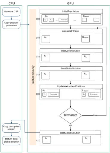
architec-ture. In order to minimize data transfer between host (CPU) and device (GPU), data of Max-CSP (the variables, their domains and the constraints) are copied in the global memory of the GPU so that all the upcoming operations can be executed in the device as described below: A random instance, called initial swarm, is first defined: nbparticles are initially set randomly in parallel to form the swarm. This is presented in the kernel InitialPopulation in Figure 3 where the kernel is launched with several blocks so that the initialization could be done in parallel for all the particles. Then, the objective function of each particle is calculated using a block like it is shown in kernel CalculateFitness of the Figure 3. Since one particle treatment, whether it’s the initial random selection of its position or its objective function evaluation, is independent from another, we have resorted to parallel computing. The evaluation of the Fit-ness function is based on template concept11. Every particle has its owntemplatewhich is an array that has a size
equal to the number of variables. An element of the arraytemplatepis called weight and it represents the number of constraints violated by variablepwhich corresponds to the positionpof the particle. For each particle, the operation first starts by initialize all the weights to zero, then, it checks the violation of constraints. For a violated constraintCi, all weights of the particles involved in this constraint are incremented by 1 and this process will be repeated for all constraints. A sample of template calculation is shown in the Figure 2:positioni2of the given instantiation of particle
iis equal to 2. It violates 2 constraintsC1andC3. Sotemplatei2will be equal to 2. Thereafter, each particle updates
its best local position (kernel BestLocalSolution in Figure 3). At the first iteration, every particle best local postion is its initial random position. Then the best global position have to be determined (kernel BestGlobalSolution in Figure 3). Afterward, each particle executes its PSO algorithm to calculate the new velocity using Equation (1) as well as its new position using Equation (2) (kernel UpdateVelocities-Positions in Figure 3). Once the position is updated, the particle recalculates its objective function, according to its new position. This process keeps repeating until one stopping criterion is attained which could be either reaching the maximum iterations number or finding the optimal solution (no constraint is violated). Each particle saves its best local solution at every iteration.
Every dimension of this particle is, so, associated to a thread of this block. We made this choice becauseX,V and
XPbestare large size dimension vectors. The components xi j∀iand j(respectivelyvi j andxPbesti j) of the verctorX
(respectivelyV andXPbest ) undergo the same treatment and each one is independent from the others. Thus the
inde-pendence of these components justify our choice. The flowchart of our GPU-PSO in CUDA is presented in Figure 3.
Fig. 2. Template Example in PSO algorithm for CSPs
4.2. Our second parallel PSO approach: GPU distributed PSO for Max-CSPs (GPU-DPSO)
The overall idea of our second proposed approach to solve Max-CSPs using GPU is based on the implementation
of the D3GPS O, described in section 3.1, in GPU architecture with appropriate modifications. The first steps of
GPU-DPSO and GPU-PSO are the same. The difference appears just after the calculation of the objective function
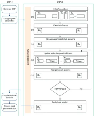
for each particle. In fact, after this computation, the swarm that consist of the initial particles, will be partitioned into separate sub-swarms in such a way that each one contains particles that violate the same number of constraints i.e having the same Fitness value (kernel GroupingParticlesInSub-Swarms in Figure 4). Then, each particle in the sub-swarms updates its velocity, its position, its best local position and then it calculates its new Fitness (kernel
UpdateVelocitiesPositionsFitness in Figure 4). Afterwards the different sub-swarms exchange particles after each
iteration of the algorithm: the sub-swarms, having particles that change Fitness during a new generation, i.e the calculation of the new Fitness gives a value other than that of the sub-swarm to which it belongs, send these particles to the appropriate sub-swarms, more specifically, to those whose Fitness is equal to the new Fitness particles no longer part of their initial groups. If the corresponding sub-swarm does not exist, it will be created to gather the related particles (kernel ReorganiseSub-swarms in Figure 4). This process continues until reaching one of the following stopping criteria: Given a number of maximum generations or finding an optimal solution (no constraint is violated). If none of the sub-swarms meets a particle that satisfy all constraints at the end, the best particle of each sub-swarm is selected in order to determine the final best solution. Thus, the program determines the best among these particles (violating the minimum number of constraints).
4.2.1. Cuda implementation
The implementation of GPU-DPSO ought to be designed in a manner that each sub-swarm is associated with one block of threads and each thread of this block is assigned to a particle from the sub-swarm. In this case, the number of particles belonging to a sub swarm should not exceed the maximal number of threads per block (which is 1024 in our GPU architecture). In order to overcome this limitation, a sub-swarm must be associated with an appropriate number of blocks of threads. The flowchart of GPU-DPSO is shown in Figure 4.
5. Experimentations
In this section, we compare between different algorithms. First we compare between PSO algorithm for Max-CSPs that we implemented on CPU, called CPU-PSO, and our GPU-PSO. Then we will compare our two proposed parallel PSO approaches GPU-PSO and GPU-DPSO to each other. For the experiments we used an Intel core i7-2630QM (2.0 Ghz) and an NVIDIA GeForce GT 525M card.
5.1. Experimental Model
As part of this work, we choosed to validate our approaches on randomly generated CSPs9in order to consider all
CSPs types : easy, hard and transition phase CSPs9. So we need to implement a random CSP generator9, to which
we apply our proposed PSO approaches. A CSP is generated in two steps: the first is to generate variables and their domain sizes and values (the domain size is randomly generated for each variable). The second is to generate binary constraints defined in extension (expressed as a set of allowed tuples i.e. the assignments combination of the variables satisfying the constraint).
The standard CSP parameters responsible to lead the generation are: the number of variables (n), their domain size (d), the constraint density p (a number between 0 and 1 indicating the ratio between the number of effective constraints to the total number of all possible constraints i.e, the probability that a constraint exists between two variables) and the constraint tightness q (a number between 0 and 1 indicating the ratio between the number of pairs of forbidden values (not permitted) by the constraint, i.e the probability for a tuple to be expected). See Algorithm 2.
Algorithm 2CSPs random generator algorithm
//generate variables
for 1toVariableNbrdo
pick randomly variable’s domain size pick randomly variable’s domain values
end for
//generate constraints
for every variables i and j/1<i< j<ndo
pick randomly x from [0..1]
ifxconstraint density then
Ci jinitially creates empty
forevery((i,a),(j,b))∈Di∗Dj do pick randomly y from [0..1]
ifyconstraint tightness then
((i,a),(j,b))⊂Ci j
end if end for end if end for
To test our algorithms, we use the following numerical values for all upcoming experiments:
variables number=40, maximal domain size of each variable=40 . For the connectivity and the tightness we choose the following values: 0.1, 0.3, 0.5, 0.7 and 0.9. So we obtain 25 density-tightness combinations. For each combination, 30 random examples are generated, which gives the total of 750 examples. For each combination density-tightness, we take the average of the 30 generated examples without considering outliers.
population is 1000.
We mention that the choice of the adequate parameters depends on the problem and is related to its real context. It can be a research apart. In order to make a quick and concise comparison between the executions of the different approaches, we are going to evaluate the performances according to the following two measurements:
• Execution time: the time laps needed to solve problems. It emphasizes time complexity. • Fitness: The number of violated constraints. It reflects solution quality
5.2. Comparative results between CPU-PSO and our GPU-PSO
For the purpose of evaluating the performances of the two algorithms: CPU-PSO and GPU-PSO, we made some comparisons between both of them. Two measures are typically used: The time spent from the beginning of the first generation until obtaining the final best solution and the quality of solution (Fitness).
To perform an experimental comparison of the two algorithms, we calculate ratios of CPU-PSO and GPU-PSO using the run time and the Fitness value as follows:
• Execution time Ratio=CPU-PSO execution time/GPU-PSO execution time. • Fitness ratio=Fitness of CPU-PSO/Fitness of GPU-PSO.
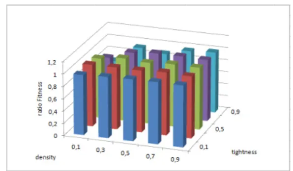
Hereby, if the ratio we have for both execution time or Fitness is superior to 1 then the GPU-PSO is better than CPU-PSO. The results show that the Fitness ratio is usually equal to 1 which has an average equal to 0.95 , Figure 6. The second ratio, which is execution time ratio, is always superior to 1. Proceeding from figure 5, we could distinguish 3 zones according to constraint density values. The first zone depicts density values belonging to [0.1,0.3] and represents easy problems. The average of execution time ratios in this zone is equal to 3.04. The second zone include density values from 0.3 to 0.7 and it represents transition phase which is the bridge between easy and hard problems. The average of execution time ratios is 3.35. The last one contains the values belonging to [0.7 , 0.9] and represents hard problems. It has an average of execution time ratios equals to 3.79. In this last zone, CPU-PSO takes up to 4.6 times more than GPU-PSO. Finally, according to these results, we conclude that the hard the CSP problem is, the more efficient the use of GPU will be. Simply when we face a large size problem the use of GPU is not only more adequate but also beneficial regarding the execution time. It is due to its high parallel computing capabilities.
Fig. 5. Execution time ratios of CPU-PSO and GPU-PSO Fig. 6. Fitness ratios of CPU-PSO and GPU-PSO
5.3. Comparative results between GPU-PSO and GPU-DPSO
In this section, the GPU-DPSO will be compared to the GPU-PSO which already has presented good results comparing to CPU-PSO.
To compare the two approaches, we used the same ratio that we used in our previous comparisons: • Execution time ratio=GPU-PSO Execution time/GPU-DPSO Execution time
• Fitness ratio=GPU-PSO Fitness/GPU-DPSO Fitness
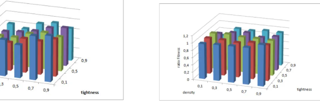
The Figures 7 and 8 represent respectively the execution time ratios and the Fitness ratios. The execution time ratio is always greater than 1 for all tightness-density combinations. the average of this ratio is 1.318, which shows that the GPU-DPSO algorithm requires less time than the GPU-PSO algorithm to run.
The average of Fitness ratio is approximately 1. This means that, comparing to GPU-PSO, the quality of solution is preserved.
So, we can conclude that GPU-DPSO algorithm allows to achieve better performances compared to GPU-PSO al-gorithm. Which is related to the choice of grid and blocks of threads sizes. In fact, the difference between the two approaches lays on the selection of the grid and blocks sizes to process the kernels of PSO algorithm in parallel: In the GPU-PSO approach, each particle is launched in a block of threads, and each thread of this block is responsible for the calculations of a dimension of the particle. For the GPU-DPSO approach, each sub swarm is assimilated to a block of threads, and every particle of this group is associated with a thread of the corresponding block.
The blocks are independently executed in no particular order. The number of grid blocks processed in parallel depends on the data to be handled: in a single multiprocessor, one or more blocks of threads can be launched according to data to be processed. As thread blocks terminate their execution, new blocks are launched on the vacated multiprocessors. In some cases, when many resources are required, the smaller the blocks are, the faster the calculation will be. In our case, GPU-PSO requires more blocks number than the GPU-DPSO, and every block requires many resources to save the appropriate data because of the large size of the CSP. Therefore, GPU-DPSO reveals better results than GPU-PSO in term of execution time.
Fig. 7. Execution time ratios of GPU-PSO and GPU-DPSO Fig. 8. Fitness ratios of GPU-PSO and GPU-DPSO
6. Conclusion
Constraint satisfaction problems are subject to intense research in both artificial intelligence and operational re-search. Unfortunately, these problems are NP-hard. Therefore, new methods are adopted for their resolution. Among these methods we mention metaheuristics such as particle swarm algorithm. However, even with the classical PSO and distributed PSO algorithms of the literature, the resolution of CSPs leads to a combinatorial explosion in the case of hard CSPs. This reveals the importance of our work, where, we have implemented two parallel PSO algorithms to improve the efficiency and robustness of CSPs, thanks to the use of high performance computing.
The highly parallel computing based on GPU was recently revealed as an effective way to exploit the large amount of available resources. However, the operation of parallel models is not obvious and several difficulties related to the execution context of this architecture shall be considered.
In this article, we have developed two parallel PSO algorithms on the hierarchical GPU. The implemented algo-rithms are experimentally applied to Max-CSPs and experiments revealed the effectiveness of GPU in the resolution. Further works could be considered by using our proposed GPU-PSO approaches to solve other CSPs extensions. Be-side comparing the GPU-DPSO with the The Dynamic Distributed Particle Swarm Optimization Algorithm based on multi-agent system. No doubt further refinement of our approaches would allow their performances to be improved.
Acknowledgment
We want to thank the reviewers for their wise comments to progress our paper.
References
1. Bouamama.S, A new distributed particle swarm optimization algorithm for constraint reasoning, Proceedings of the 14th international confer-ence on Knowledge-based and intelligent information and engineering systems: Part II, September 08-10, 2010, Cardiff, UK
2. Bouammama.S, Ghedira K.: A Dynamic Distributed Double Guided Genetic Algorithm for Optimization and Constraint Reasoning; Interna-tional Journal of ComputaInterna-tional Intelligence Research; Vol 2, Issue 2, pp. 181-190, (2006).
3. Brodtkorb.A, Dyken.C, Hagen.T. Hjelmervik.J. Storaasli.O: State-of-the-art in heterogeneous computing. Sci. Program. 18(1) (2010) 4. Freuder.E.C, Wallace.R.J : Partial constraint satisfaction. Articial Intelligence, 58(1-3) :2170, 1992.
5. Kennedy. J, and Eberhart.R.C : Particle Swarm Optimization. Proc. of IEEE International Conference on Neural Network, Piscataway, NJ. Pp.. 1942-1948 (1995).
6. Luong.T.V, Melab.N, Talbi.E.G : GPU-based Island Model for Evolutionary Algorithms. Genetic and Evolutionary Computation Conference (GECCO), Portland, US, 2010
7. Nickolls.J and Dally.W.J : the GPu Computing Era, IEEE Micro, vol. 30, no. 2, 2010, pp. 5669. 8. NVIDIA, NVIDIA CUDA Programming version 6.0, 2014.
9. Smith B.M. :The Phase Transition and the Mushy Region in Constraint Satisfaction Problems, Actes de the 11th European Conference On Artificial Intelligence ECAI94, A.G. Cohn, Amesterdam, The Netherlands, 1994, p. 100-104.
10. Tsang E.P.K. : Foundations of Constraints Satisfaction, Academic Press Limited, UK, 1993.
11. Tsang E.P.K, Wang C.J., Davenport A., Voudouris C., Lau T.L.: A family of stochastic methods for Constraint Satisfaction and Optimization. Technical report, University of Essex, Colchester, UK, November (1999).
12. Y. Shi, R. Eberhart : A Modied Particle Swarm Optimizer, in Proceedings of the IEEE Congress on Evolutionary Computation, May 1998, pp. 6973.
13. Zhou.Y, Tan.Y : GPU-based parallel particle swarm optimization. IEEE Congress on Evolutionary Computation, 2009. CEC ’09, pp. 1493-1500, 2009.