Statistics Preprints Statistics
8-2010
Bayesian Methods for Estimating the Reliability of
Complex Systems Using Heterogeneous Multilevel
Information
Jiqiang Guo
Iowa State University, [email protected]
Alyson G. Wilson
Iowa State University, [email protected]
Follow this and additional works at:http://lib.dr.iastate.edu/stat_las_preprints Part of theStatistics and Probability Commons
Recommended Citation
Guo, Jiqiang and Wilson, Alyson G., "Bayesian Methods for Estimating the Reliability of Complex Systems Using Heterogeneous
Multilevel Information" (2010).Statistics Preprints. 104.
Bayesian Methods for Estimating the Reliability of Complex Systems
Using Heterogeneous Multilevel Information
Abstract
We propose a Bayesian approach for assessing the reliability of multicomponent systems. Our models allow us to evaluate system, subsystem, and component reliability using the available multilevel information. Data are collected over time, and include pass/fail, lifetime, censored, and degradation data. We illustrate the
methodology through an example and discuss how to extend the approach to more complex systems. Keywords
degradation, hierarchical model, lifetime, multi-component system, system reliability Disciplines
Statistics and Probability Comments
This preprint was published as Jiqiang Guo & Alyson G. Wilson, "Bayesian Methods for Estimating System Reliability Using Heterogeneous Multilevel Information",Technometrics(2013): 461-472, doi:10.1080/ 00401706.2013.804441.
Preprint # 10–10
Bayesian Methods for Estimating the
Reliability of Complex Systems Using
Heterogeneous Multilevel Information
Jiqiang Guo
[email protected]
Department of Statistics
Iowa State University
Ames, Iowa, 50011
Alyson G. Wilson
[email protected]
Department of Statistics
Iowa State University
Ames, Iowa, 50011
August 8, 2010
ABSTRACT
We propose a Bayesian approach for assessing the reliability of multi-component systems. Our models allow us to evaluate system, subsys-tem, and component reliability using the available multilevel informa-tion. Data are collected over time, and include pass/fail, lifetime, cen-sored, and degradation data. We illustrate the methodology through an example and discuss how to extend the approach to more complex systems.
KEY WORDS: Degradation, Hierarchical model, Lifetime, Multi-component system, System reliability
1.
INTRODUCTION
This paper proposes methodology to integrate system, subsystem, and com-ponent data to assess system reliability as it changes over time. The approach addresses two common problems in reliability: estimating how reliability changes over time and using information from multiple levels in the system to make inference. Generalizing previous work (Johnson et al. 2003; Reese et al. 2009), we discuss models for pass/fail, lifetime, degradation, and expert opinion data at any system level.
Bayesian methods are appealing for this problem due to their natural incorporation of expert opinion, and a variety of approaches have been pro-posed in the literature. For example, considering only pass/fail data, Mastran (1976); Mastran and Singpurwalla (1978) describe a procedure to approxi-mate the posterior mean reliability of a coherent system using test and prior data at both the component and system level. Martz et al. (1988); Martz and Waller (1990) propose a bottom-up approach for approximating the pos-terior distribution of reliability of series and parallel systems of independent Binomial subsystems and components. Tang et al. (1997) proposes methods to obtain the exact posterior distributions in special cases. Johnson et al. (2003) develops full simultaneous Bayesian for pass/fail data collected at any level of the system over time.
Extending beyond pass/fail data, Thompson and Chang (1975) and Chang and Thompson (1976) consider first the reliability of subsystems with one or
more components in series, where each component has an independent ex-ponential distribution, and then compute Bayesian credible intervals for ar-bitrary series-parallel system comprised of these subsystems. Winterbottom (1984) surveys classical and Bayesian results for estimating system reliability from Binomial and exponential component data in coherent systems. Robin-son and Dietrich (1988) consider component-level data with exponential life-times that have decreasing failure rates as the system develops. Sharma and Bhutani (1994) estimate the availability of series and parallel systems where the components have exponential time to failure and repair. Bergman and Ringi (1997a) consider dependence between components induced by com-mon operating environments; Bergman and Ringi (1997b) use data from non-identical environments. Hulting and Robinson (1994) is an exception to the above approaches, as they generalize the results of Martz et al. (1988) to make approximate inferences about the reliability of the system using multi-level information. They approximate the reliability for a series sys-tem using non-homogeneous Poisson processes to model the repair histories of repairable subsystems and time-to-failure data (modeled with a Weibull distribution) for nonrepairable subsystems.
In the last decade, Markov chain Monte Carlo (MCMC) has made fully Bayesian methods possible for addressing system reliability problems. For example, Johnson et al. (2003) and Hamada et al. (2004) propose fully Bayesian approaches for simultaneously estimating the reliability for a sys-tem and its subsyssys-tems/components described by a fault tree using pass/fail
data. Wilson and Huzurbazar (2007) considers a system represented by a Bayesian network (BN), similarly with pass/fail data. Wilson et al. (2006) and Hamada et al. (2008) propose approaches for assessing system reliability with pass/fail data at the system, and pass/fail, lifetime, or degradation data at the components. Reese et al. (2009) considers lifetime data throughout the system. This paper discusses a unified fully Bayesian approach for si-multaneously estimating system, subsystem, and component reliability when there are pass/fail, lifetime, degradation, or expert judgment data at any level of the system.
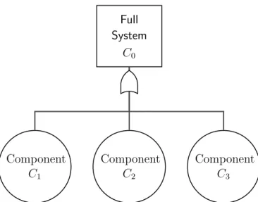
We develop this methodology using a series system with three compo-nents, which is represented as a fault tree in Figure 1. In Section 2, we introduce the models. In Section 3, we demonstrate the methodology by considering three scenarios applied to Figure 1. In each scenario, one com-ponent has pass/fail data collected over time, one has lifetime data, and one has degradation data; Scenario 1 has pass/fail data collected over time at the system, Scenario 2 has lifetime data at the system, and Scenario 3 has degradation data at the system. In Section 4, we discuss extensions of the methodology.
Full System C0 Component C1 Component C2 Component C3
Figure 1: Three-component series system.
2.
MODEL SPECIFICATION
In our development, we assume a coherent system represented by a fault tree. The fault tree describes the relationships between different level of failure events. We call those events requiring no further decomposition basic events
and others simply non-basic events. Label each event Ci (i = 0,1,2,3, . . .).
In Figure 1, for example, C0 denotes the system (a non-basic event) and C1, C2, C3 denote the three components (basic events). For any event Ci, let Ri(t|Θi) denote its reliability function at timet given parameters Θi. LetTi
be the random variable associated with the lifetime of Ci, with probability
density functionfi(t|Θi) and cumulative distribution functionFi(t|Θi). We
By definition, we have the following relations: Ri(t|Θi) = Pr{Ti > t|Θi}= 1−Fi(t|Θi), (1) and fi(t|Θi) = dFi(t|Θi) dt = d 1−Ri(t|Θi) dt =− dRi(t|Θi) dt . (2)
As a result, for Ci, eitherRi(t|Θi) or fi(t|Θi) is sufficient to determine the
other. We call the lifetime distribution determined by the reliability function the induced lifetime distribution.
The first step of model development is specifying the reliability function
Ri(t|Θi), which is specified directly or induced from the probability
den-sity function fi(t|Θi). The second step is to use the system structure to
determine the reliability functions for all of the non-basic events. Lifetime distributions for each event follow from the reliability functions. If the non-basic events have lifetime or pass/fail data, their likelihood functions are straightforward. If there are degradation data observed for the non-basic events, we specify the likelihoods with constraints determined by their reli-ability functions. Finally, the data for all events can be combined to model the system and estimate reliabilities.
For example, consider the system in Figure 1. The first step, modeling the three basic events, is detailed in Section 3. In the second step, since the system works if and only if all three components work, the reliability function
of system is the product of the reliability functions of the three components. That is,
R0(t|Θ0) = R1(t|Θ1)·R2(t|Θ2)·R3(t|Θ3). (3)
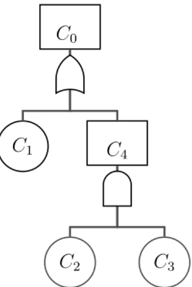
Another example of expressing the reliability of a system/subsystems in terms of basic events concerns the system in Figure 2. By virtue of the system structure, we can obtain the reliability functions of non-basic events as follows (parameters Θi’s are suppressed):
R4(t) = 1−(1−R2(t))(1−R3(t)) =R2(t) +R3(t)−R2(t)R3(t), (4) R0(t) =R1(t)R4(t) =R1(t)R2(t) +R1(t)R3(t)−R1(t)R2(t)R3(t). (5)
C
0C
1C
4C
2C
3Figure 2: Another fault tree system: C4 works if at least one of C2 and C3
2.1
Pass/fail data
Suppose at timesij (j = 1, . . . , ni),Nij tests have been conducted onCi, with bij passing the test. Denote the data vector as bi. The likelihood function
for a basic event, using the Binomial distribution is given as
Li(bi|Θi) = ni Y j=1 Nij bij Ri(sij|Θi) bij 1−Ri(sij|Θi) Nij−bij . (6)
The reliability function in (6) can take many forms. Consider, for exam-ple, a Logit model, where we specify the reliability function as
Ri(t|Θi) = logit−1(θi+ηit), θi >0, ηi <0, Θi = (θi, ηi), (7)
where logit−1 is the inverse of Logit function which is defined as logit(x) = logx−log(1−x), 0< x < 1.
The reliability function Ri(t) for a non-basic event is determined by the
system structure. In particular, Ri(t) is a function of the reliabilities of basic
events as illustrated by (3) for the system in Figure 1.
2.2
Lifetime data
For lifetime data, let ti =ti1, ti2, . . . , timi be the lifetime data collected for
likelihood Li(ti|Θi) = mi Y j=1 fi(tij|Θi). (8)
The likelihood is easy to generalize to censored data, with details given in Section 4.
The probability density functionfi(t) for a basic event depends on which
model is used. As for a non-basic event, the density function can be derived from its reliability function. For the system in Figure 1, by using the re-lationship of (2), the density function for the lifetime of C0 can be derived
from (3).
2.3
Degradation Data
Degradation data measure some quantity about a component or subsystem that is indirectly related to reliability. In particular, degradation data are typically thought of a continuous quantity that changes over time, with fail-ure occurring when the quantity passes some threshold.
Consider degradation data for event Ci, and suppose that we have
mea-sured a total vi different units. Denote the time of the measurements, dijk,
as qijk, where j = 1, . . . , vi and k = 1, . . . , zij. That is, for each of the vi
units, we measure the degradation quantity zij times. Let Dijk denote the
random variables associated with the degradation quantities dijk.
model: specifically, the reliability is the probability that the degradation quantity is above the threshold at time t. For example, consider the degra-dation process as in specified in Wilson et al. (2006):
Dijk ∼Normal(αi−βij−1qijk, σi2), αi >0, βij >0, σi >0. (9)
That is, all events are identical at t = 0, but they each degrade at their own rates. Let di denote the degradation data for Ci. We can construct a
likelihood function using (9):
Li(di|βi, αi, σi) = vi Y j=1 zij Y k=1 1 σi φ dijk−αi+β −1 ij qijk σi ! , (10)
whereφ(·) is the probability density function of standard normal distribution. To connect the degradation model with the lifetime distribution and re-liability function, let τi be the threshold of the degradation process. This
event fails when the degradation quantity is less than τi. Then we have
Tij = inf{t≥0 :αi−βij−1t ≤τi}= (αi−τi)βij, αi > τi >0. (11)
Suppose that we further assume that logβij ∼ Normal(µi, ψ2i). Then
the lifetime of the event has a Log-normal distribution. That is, logTij ∼
is Ri(t|Θi) = 1−Φ logt−µi−log(αi−τi) ψi , Θi = (µi, ψi, αi, τi, σi), (12)
where Φ(·) is the cumulative distribution function of standard normal distri-bution.
For non-basic events, we first derive the induced lifetime distribution as described in Section 2. If we further assume the same degradation model as (9), the distribution of (αi −τi)βij in (11) is determined for the non-basic
event. In our Bayesian model, we must choose our prior distribution for (αi, τi, βij) such that the distribution of (αi−τi)βij is the same as the induced
lifetime distribution for eventCi. One simple way to achieve this is to specify
the following conditional probability density distribution function for βij in
terms of the induced lifetime distribution fi(t|Θi):
gi(βij|Θi) = (αi−τi)fi
βij(αi−τi)|Θi
. (13)
This specification forβij, along with any proper prior distributions forαi and τi, makes the distribution of (αi−τi)βij coincide with the induced lifetime
distribution. Consequently the likelihood function for a non-basic event ac-cording to the above model specification still has the form of (10), but with constraints on βij from lower-level events.
2.4
Prior Information
Specifying prior distributions in a Bayesian context is also part of the model-ing process. An advantage of Bayesian methodology is that we can incorpo-rate “non-data” information into our models; for example, information from expert opinions, historical data, and from similar systems.
Initial specification of prior distributions for the parameters describing basic events follows standard Bayesian practice. However, some thought must be given to the specification of prior distributions for the degradation data. Suppose that we are working with the model (9). Consider the specification of the priors for the degradation quantity at time 0, αi and the threshold τi,
both of which are assumed to be positive. We consider two approaches. A first approach, which is mentioned in Wilson et al. (2006), is to specify a Gamma prior distribution on αi and then Beta distribution on τi/αi given αi. This approach is useful if we want to impose non-informative priors on τi or on both αi and τi.
As an example, suppose that we specify the following Gamma prior dis-tribution on αi and uniform distribution on τi/αi givenαi:
αi ∼Gamma(ναi, ξαi), τi|αi ∼Uniform[0, αi]. (14)
(Note that our Gamma distribution has a parameterization such that the above specification for αi has mean ναi·ξαi.)
to specify an informative prior for τi. This can be difficult to specify using
the preceding approach. However, consider the following. We specify an informative prior for τi and then a conditional prior distribution forαi given τi. An example using Gamma distribution is given as follows:
τi ∼Gamma(ντi, ξτi); (αi−τi)|τi ∼Gamma(ναi−τi, ξαi−τi). (15)
Specifying prior distributions for non-basic events requires additional thought. Recall that the reliability and lifetime of non-basic events are func-tions of the parameters of the basic events and the degradation model have constraints from lower level events. This implies for non-basic events, we need to specify prior distributions on functions of parameters. In addition, the prior distributions specified on the parameters of basic events induce
prior distributions on the reliability and lifetime of non-basic events. Conse-quently, if we also have prior information about the reliability or lifetime of non-basic events, we need a way to combine the information.
We use the Bayesian melding approach proposed in Poole and Raftery (2000). Suppose that we have independent prior distributions on parameters θ and φ = M(θ), q1(θ) and q2(φ). M(·) is a deterministic function. The
prior on θ induces a prior on φ=M(θ), denoted by q1∗(φ).
Poole and Raftery (2000) proposes pooling q∗1(φ) and q2(φ) and then
with its formula given by ˜ q(θ)∝q1(θ) q2(M θ) q∗ 1 M(θ) !1−α , (16)
where α is the pooling weight.
In our system reliability setting, the reliability on a non-basic event at some time is a function of parameters of lower level events. Using the above notation, we have initial priors of the basic events that is denoted by q1(θ)
and initial priors on some reliability function of non-basic events that is denoted by q2(φ). Thenq1∗(φ) is the prior induced byq1(θ) on the reliability
function. And ˜q(θ) is the final prior on the parameters of basic events after melding. As a result, if we elicit the prior information on non-basic events as prior on the reliability, we can use the Bayesian melding approach to combine prior information given at the basic and non-basic events.
3.
THREE-COMPONENT SERIES
SYSTEM SCENARIOS
In this section, we apply the proposed methodology to analyze the three component system pictured in Figure 1. The system is composed of three components, and the system works if and only if the three components work. We denote the system by C0 and the three components by C1, C2, and C3.
Using the notation from Section 2, we have
R0(t|Θ0) = R1(t|Θ1)·R2(t|Θ2)·R3(t|Θ3), (17)
where Θ0 includes Θ1,Θ2,Θ3 and any other parameters involved in
model-ing the system. Note that by assumption, all the reliability functions are differentiable with respect to t and their parameters.
We consider three scenarios for the system. Each scenario has the same information for the components: pass/fail data for C1; lifetime data for C2;
and degradation data for C3. The degradation data for C3 are collected for
20 units that are measured one time each. The component data are given in Table 1.
Scenario 1 has pass/fail data collected over time at the system, Scenario 2 has lifetime data at the system, and Scenario 3 has degradation data at the system. The system data are given in Table 2. The degradation data for the system are collected for five systems that are measured eight times each across different ages.
We first analyze the three scenarios when there is no prior information for the system. We then introduce prior information for the system and use Bayesian melding to reanalyze Scenario 1.
Table 1: Pass/fail data for component 1 (number of pass out of total), lifetime time (years) data for component 2, and degradation data for component 3. In the parenthesis is the age (years) when it is tested or measured.
C1 25/25 (0), 25/25 (4), 25/25 (8), 24/25 (12), 22/25 (16), 23/25 (20), 20/25 (24), 14/25 (28), 9/25 (32), 7/25 (36), 3/25 (40) C2 23.8, 45.49, 64.61, 38.77, 11.22, 58.25, 29.93, 51.56, 75.42, 43.85, 44.01, 26.47, 26.9, 45.03, 21.11, 72.81, 64.04, 86.37, 56.67, 51.86, 69.88, 26.49, 71.24, 52.7, 67.84 C3 93.61 (2), 95.80 (4), 80.59 (6), 83.79 (8), 80.25 (10), 54.60 (12), 70.20 (14), 58.06 (16), 38.63 (18), 26.18 (20), 87.93 (2), 85.44 (4), 86.31 (6), 71.48 (8), 70.73 (10), 57.85 (12), 60.43 (14), 70.45 (16), 40.88 (18), 51.15 (20)
Table 2: System data for the three scenarios: Pass/fail data (number of pass out of total) with ages indicated in the parenthesis, lifetime time (years) data, and degradation data for five systems (every consecutive eight are the measurements for each system at different ages showed in the parenthesis).
Pass/Fail 20/20 (0), 20/20 (2), 20/20 (4), 20/20 (6), 20/20 (10), 18/20 (15), 16/20 (20), 4/20 (30) Lifetime 30.2, 36.55, 25.11, 39.35, 27.57, 25.91, 31.5, 29.24, 18.39, 16.65, 21.85, 24.88, 31.61, 18.74, 19.63, 28.98, 11.1, 21.66, 22.41, 26.04, 25.07, 23.48, 28.21, 25.21, 25.12, 27.76, 23.47, 23.51, 24.39, 21.93, 37.63, 20.32, 28.17, 24.66, 30.13, 21.42, 17.21, 19.98, 33.09, 16.04, 17.96, 19.57, 22.91, 25.69, 23.47, 16.91, 27.2, 27.23 Degradation 168.96 (2), 183.06 (4), 143.02 (8), 136.58 (12), 100.32 (16), 74.63 (20), 72.38 (24), 33.29 (28) 203.23 (2), 177.13 (4), 159.21 (8), 125.13 (12), 93.56 (16), 106.83 (20), 66.76 (24), 37.06 (28) 190.68 (2), 178.63 (4), 174.95 (8), 142.19 (12), 125.78 (16), 85.48 (20), 86.96 (24), 65.61 (28) 201.76 (2), 184.75 (4), 144.21 (8), 154.4 (12), 123.1 (16), 100.9 (20), 97.86 (24), 67.54 (28) 179.3 (2), 168.64 (4), 168.86 (8), 134.18 (12), 136.34 (16), 98.92 (20), 66.5 (24), 48.96 (28)
3.1
Models
We use the Logit model (Section 2.1) forC1, the Weibull lifetime distribution
model (Section 2.2) for C2, and the degradation model (Section 2.3) for C3. For the system (C0), the reliability function is determined from the
specifications for the components, as discussed in Section 2.
The three reliability functions forC1, C2, and C3 are given below.
R1(t|Θ1) = logit−1(θ1+η1t), Θ1 = (θ1, η1), (18) R2(t|Θ2) = exp " − t λ2 δ2# , Θ2 = (δ2, λ2), (19) R3(t|Θ3) = 1−Φ logt−µ3−log(α3−τ3) ψ3 , Θ3 = (µ3, ψ3, α3, τ3, σ3). (20)
Using (17), the reliability function for the system is
R0(t|Θ0) = logit−1(θ1+η1t)·exp " − t λ2 δ2# · 1−Φ logt−µ3−log(α3−τ3) ψ3 . (21)
Let b1 denote the data for C1; t2 for C2; d3 for C3; b0, t0, and d0 for C0. Additionally,β3 ={β3j :j = 1, . . . , v3}, β0 ={β0j :j = 1, . . . , v0}.
In Scenario 1, with pass/fail data at the system, (21) specifies the prob-ability of observing a “pass” at time t. For example, we have observed 16 passes out of total 20 tests when t = 20. The likelihood term for these 20
tests is given by 20 16 R0(20|Θ0) 16 1−R0(20|Θ0) 4 ,
where R0(20|Θ0) is given in (21) witht = 20.
In Scenario 2, with lifetime data at the system, the probability density function for the system lifetime distribution is determined by (21). Following (2), we have
f0(t|Θ0) = −
dR0(t|Θ0)
dt , (22)
where R0(t|Θ0) is given in (21). Since the data in Table 2 are independent,
we have L0(t0|Θ0) = 48 Y j=1 f0(t0j|Θ0),
where for example t01= 30.2 and t02= 36.55.
In Scenario 3, with degradation data at the system, assume that we are modeling the data using the degradation model from Section 2.3. Following (10), we have the likelihood function:
L0(d0|β0, α0, σ0) = v0 Y j=1 z0j Y k=1 1 σ0 φ d0jk−α0 +β −1 0j q0jk σ0 ! ,
according to equation (13). That is, g0(β0|Θ0) = (α0−τ0)f0 β0(α0−τ0)|Θ0 , (23)
where f0(· |Θ0) is given in (22) such that the reliability function for the
system still satisfies (17).
3.2
Prior distributions
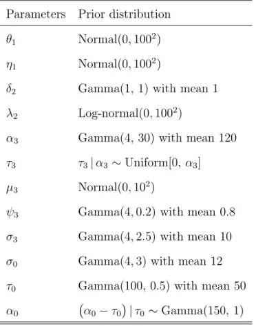
When specifying prior distributions, we have the parameters from the basic events: θ1, η1, δ2, λ2, α3, τ3, ψ3, µ3, σ3. In Scenario 3, we also have α0, τ0, σ0. In real applications, these parameters are elicited; for illustration, we use
fairly diffuse priors for some parameters here. These priors are detailed in Table 3. The priors for α3, τ3, α0, and τ0 follows the discussion in Section
Table 3: Prior distributions Parameters Prior distribution
θ1 Normal(0,1002) η1 Normal(0,1002)
δ2 Gamma(1, 1) with mean 1
λ2 Log-normal(0,1002)
α3 Gamma(4, 30) with mean 120
τ3 τ3|α3 ∼Uniform[0, α3] µ3 Normal(0,102)
ψ3 Gamma(4,0.2) with mean 0.8 σ3 Gamma(4,2.5) with mean 10
σ0 Gamma(4,3) with mean 12
τ0 Gamma(100, 0.5) with mean 50 α0 α0−τ0
|τ0 ∼Gamma(150,1)
3.3
Joint Posterior Distribution
LetL1(b1|Θ1) be the likelihood function for component 1 (from (6));L2(t2|Θ2)
be the likelihood function for component 2 (from (8)); andL3(d3|Θ3) be the
likelihood function for component 3 (from (10)). The likelihood function for the systemL0 is given above. By Bayes’ theorem, we obtain the following
un-normalized probability density functions for the joint posterior distribution for the three scenarios.
The unnormalized joint posterior probability density function for Scenario 1 is given by π(Θ0,β3|b1,t2,d3,b0) ∝L1(b1|Θ1)L2(t2|Θ2)L3(d3|β3,Θ3)L0(b0|Θ0) · v3 Y j=1 β3j−1φ(logβ3j −µ3)/ψ3 (24) ·φ(θ1/100)·φ(η1/100)·exp(−δ2)·λ−21φ(logλ2/100)·φ(µ3/10)
·α33exp (−α3/30)·I(α3 > τ3 ≥0)·ψ33exp (−ψ3/0.2)·σ33exp (−σ3/2.5)
The unnormalized joint posterior probability density function for Scenario 2 is given by π(Θ0,β3|b1,t2,d3,t0) ∝L1(b1|Θ1)L2(t2|Θ2)L3(d3|β3,Θ3)L0(t0|Θ0) · v3 Y j=1 β3j−1φ(logβ3j −µ3)/ψ3 (25) ·φ(θ1/100)·φ(η1/100)·exp(−δ2)·λ−21φ(logλ2/100)·φ(µ3/10)
·α33exp (−α3/30)·I(α3 > τ3 ≥0)·ψ33exp (−ψ3/0.2)·σ33exp (−σ3/2.5)
3 is given by π(Θ0,β3,β0|b1,t2,d3,d0) ∝L1(b1|Θ1)L2(t2|Θ2)L3(d3|β3,Θ3)L0(d0|β0,Θ0) · v3 Y j=1 β3j−1φ(logβ3j −µ3)/ψ3 · v0 Y j=1 g0(β0j|Θ0) (26) ·φ(θ1/100)·φ(η1/100)·exp(−δ2)·λ−21φ(logλ2/100)·φ(µ3/10)
·α33exp (−α3/30)·I(α3 > τ3 ≥0)·ψ33exp (−ψ3/0.2)·σ33exp (−σ3/2.5)
· α0−τ0
149
exp (−(α0−τ0))·τ099exp (−τ0/0.5) ·σ03exp (−σ0/3).
3.4
Model estimation and estimated reliabilities
We can use MCMC to draw samples from the unnormalized joint posterior distributions. In particular, we used a one-variable-at-a-time random walk Metropolis algorithm to draw samples from the posterior distributions spec-ified in (24), (25), and (26).
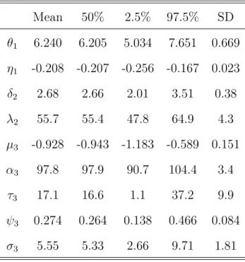
The marginal posterior distributions of the parameters are summarized in Table 4 (Scenario 1), Table 5 (Scenario 2), and Table 6 (Scenario 3).
Table 4: Empirical mean, median, 2.5% and 97.5% quantiles, and standard deviation for each variable for Scenario 1.
Mean 50% 2.5% 97.5% SD θ1 6.240 6.205 5.034 7.651 0.669 η1 -0.208 -0.207 -0.256 -0.167 0.023 δ2 2.68 2.66 2.01 3.51 0.38 λ2 55.7 55.4 47.8 64.9 4.3 µ3 -0.928 -0.943 -1.183 -0.589 0.151 α3 97.8 97.9 90.7 104.4 3.4 τ3 17.1 16.6 1.1 37.2 9.9 ψ3 0.274 0.264 0.138 0.466 0.084 σ3 5.55 5.33 2.66 9.71 1.81
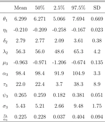
Table 5: Empirical mean, median, 2.5% and 97.5% quantiles, and standard deviation for each variable for Scenario 2.
Mean 50% 2.5% 97.5% SD θ1 6.299 6.271 5.066 7.694 0.669 η1 -0.210 -0.209 -0.258 -0.167 0.023 δ2 2.79 2.77 2.09 3.61 0.38 λ2 56.3 56.0 48.6 65.3 4.2 µ3 -0.963 -0.971 -1.206 -0.674 0.135 α3 98.4 98.4 91.9 104.9 3.3 τ3 22.0 22.4 3.7 38.3 8.9 ψ3 0.265 0.259 0.182 0.381 0.051 σ3 5.43 5.21 2.66 9.48 1.75 τ3 α3 0.225 0.228 0.037 0.404 0.094
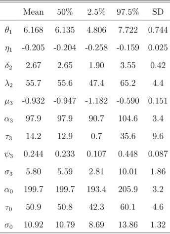
Table 6: Empirical mean, median, 2.5% and 97.5% quantiles, and standard deviation for each variable for Scenario 3.
Mean 50% 2.5% 97.5% SD θ1 6.168 6.135 4.806 7.722 0.744 η1 -0.205 -0.204 -0.258 -0.159 0.025 δ2 2.67 2.65 1.90 3.55 0.42 λ2 55.7 55.6 47.4 65.2 4.4 µ3 -0.932 -0.947 -1.182 -0.590 0.151 α3 97.9 97.9 90.7 104.6 3.4 τ3 14.2 12.9 0.7 35.6 9.6 ψ3 0.244 0.233 0.107 0.448 0.087 σ3 5.80 5.59 2.81 10.01 1.86 α0 199.7 199.7 193.4 205.9 3.2 τ0 50.9 50.8 42.3 60.1 4.6 σ0 10.92 10.79 8.69 13.86 1.32
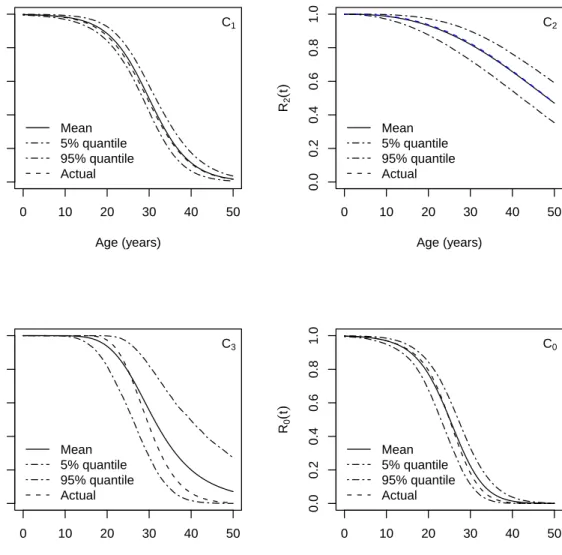
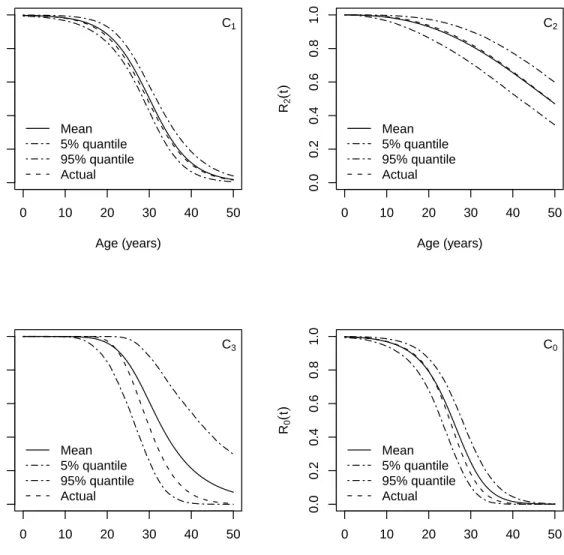
Perhaps more interesting, we can obtain the posterior distributions of the reliability functions for both the components and the system from the samples from posterior distributions. Plots for the functions with respect to time t along with a credible interval band are presented in Figure 3 (Sce-nario 1), Figure 4 (Sce(Sce-nario 2), and Figure 5 (Sce(Sce-nario 3). Note that the estimation of the reliability function of C3 is not as accurate as those forC1
and τ3 in the degradation model for C3. Recall that a failure occurs when
the degradation quantity passes the threshold. Here we have noninformative prior for the threshold τ3, so the degradation data do not give much
infor-mation about the reliability. Since we perform inference on the system as a whole, the information from the system contributes to the estimation of C3;
otherwise, we would not have information about the component reliability. Our methodology takes advantage of information at all levels to estimate the system reliability, but also it helps to estimate component reliability using data from the whole system.
0 10 20 30 40 50 0.0 0.2 0.4 0.6 0.8 1.0 Age (years) R1 ( t ) Mean 5% quantile 95% quantile Actual C1 0 10 20 30 40 50 0.0 0.2 0.4 0.6 0.8 1.0 Age (years) R2 ( t ) Mean 5% quantile 95% quantile Actual C2 0 10 20 30 40 50 0.0 0.2 0.4 0.6 0.8 1.0 Age (years) R3 ( t ) Mean 5% quantile 95% quantile Actual C3 0 10 20 30 40 50 0.0 0.2 0.4 0.6 0.8 1.0 Age (years) R0 ( t ) Mean 5% quantile 95% quantile Actual C0
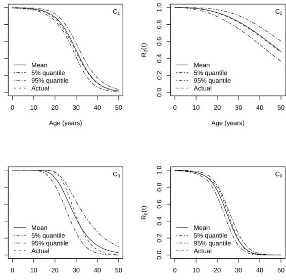
Figure 3: Reliability estimates and credible intervals with respect to the age. Upper left: Component 1, with pass/fail data using Logit model. Upper right: Component 2, with life time data assumed to have Weibull distribu-tion. Lower left: Component 3, with degradation data. Lower right: The full system, for which pass/fail data are collected.
0 10 20 30 40 50 0.0 0.2 0.4 0.6 0.8 1.0 Age (years) R1 ( t ) Mean 5% quantile 95% quantile Actual C1 0 10 20 30 40 50 0.0 0.2 0.4 0.6 0.8 1.0 Age (years) R2 ( t ) Mean 5% quantile 95% quantile Actual C2 0 10 20 30 40 50 0.0 0.2 0.4 0.6 0.8 1.0 Age (years) R3 ( t ) Mean 5% quantile 95% quantile Actual C3 0 10 20 30 40 50 0.0 0.2 0.4 0.6 0.8 1.0 Age (years) R0 ( t ) Mean 5% quantile 95% quantile Actual C0
Figure 4: Reliability estimates and credible intervals with respect to the age. Upper left: Component 1, with pass/fail data using Logit model. Upper right: Component 2, with life time data assumed to have Weibull distribu-tion. Lower left: Component 3, with degradation data. Lower right: The full system, for which lifetime data are collected.
0 10 20 30 40 50 0.0 0.2 0.4 0.6 0.8 1.0 Age (years) R1 ( t ) Mean 5% quantile 95% quantile Actual C1 0 10 20 30 40 50 0.0 0.2 0.4 0.6 0.8 1.0 Age (years) R2 ( t ) Mean 5% quantile 95% quantile Actual C2 0 10 20 30 40 50 0.0 0.2 0.4 0.6 0.8 1.0 Age (years) R3 ( t ) Mean 5% quantile 95% quantile Actual C3 0 10 20 30 40 50 0.0 0.2 0.4 0.6 0.8 1.0 Age (years) R0 ( t ) Mean 5% quantile 95% quantile Actual C0
Figure 5: Reliability estimates and credible intervals with respect to the age. Upper left: Component 1, with pass/fail data using Logit model. Upper right: Component 2, with life time data assumed to have Weibull distribu-tion. Lower left: Component 3, with degradation data. Lower right: The full system, for which degradation data are collected.
3.5
Incorporating prior information about the system
In the above analyses, we have not incorporated any additional prior infor-mation about the system. Suppose we have additional independent prior information for the system, and we believe the system reliability at age of 20 years, R0(t = 20|Θ0), has a Beta(4,2) distribution. From (21), the
sys-tem reliability R0(t = 20|Θ0) is a deterministic function of parameters of
the three components. Consequently the prior on Θ0 induces a prior on R0(t= 20|Θ0). Specifically, let q1(θ) denote the prior in (24):
q1(θ)∝φ(θ1/100)·φ(η1/100)·exp(−δ2)·λ−21φ(logλ2/100)·φ(µ3/10)
·α33exp (−α3/30)·I(α3 > τ3 ≥0)·ψ33exp (−ψ3/0.2)·σ33exp (−σ3/2.5).
(27)
q1∗(M(θ)) is the prior distribution on M(θ) induced by the specification of (27). q2[M(θ) = R0(t = 20|θ)] is the density function of the Beta(4,2)
distribution.
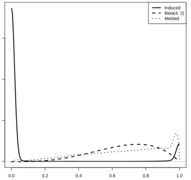
In Figure 6, we plot the induced prior q1∗(M(θ)); the initial prior on
M(θ), q2(M(θ)); and the pooling ofq1∗(M(θ)) and q2(M(θ)). Inverting the
pooled prior on M(θ) to prior on θ gives the final Bayesian Melding prior. We use the melded prior as in (24) with pooling weight α being 0.5 instead to perform our posterior inference.
0.0 0.2 0.4 0.6 0.8 1.0 0 5 10 15 R0(t=20) Density Induced Beta(4, 2) Melded
Figure 6: Probability density functions of priors on the system reliability when t = 20. The solid line represents the prior induced from the prior specified on the basic events; the dashed line Beta(4,2); the dotted line the pooled prior.
When executing the analyses, the induced prior often needs to be esti-mated numerically using, for example, kernel methods, since the determinis-tic function is complex. The MCMC can then be carried out with the updated posterior distribution. Notice that the induced prior is time-consuming to compute, and since its computation is required in every evaluation of the posterior distribution, the overall MCMC procedure can be quite slow.
First, we can approximate the induced prior distribution using a parametric form. For example, we can find a Beta distribution (or mixture of Beta distributions) to approximate the induced prior on system reliability. A second approach is to first evaluate the induced prior at multiple points (say 107 points). We can then use a “table lookup”, which returns the density of the closest point to approximate the induced prior. This is the approach we used in our computations. The estimation results are presented in Table 7 and Figure 7.
Table 7: Empirical mean, median, 2.5% and 97.5% quantiles, and standard deviation for each variable.
Mean 50% 2.5% 97.5% SD θ1 6.214 6.178 5.018 7.618 0.666 η1 -0.207 -0.206 -0.255 -0.165 0.022 δ2 2.76 2.73 2.05 3.63 0.40 λ2 55.6 55.4 47.9 64.5 4.2 µ3 -0.928 -0.942 -1.184 -0.588 0.151 α3 97.8 97.8 90.8 104.3 3.4 τ3 17.6 17.2 1.1 37.7 10.0 ψ3 0.278 0.268 0.141 0.468 0.083 σ3 5.51 5.29 2.62 9.64 1.80
0 10 20 30 40 50 0.0 0.2 0.4 0.6 0.8 1.0 Age (years) R1 ( t ) Mean 5% quantile 95% quantile Actual C1 0 10 20 30 40 50 0.0 0.2 0.4 0.6 0.8 1.0 Age (years) R2 ( t ) Mean 5% quantile 95% quantile Actual C2 0 10 20 30 40 50 0.0 0.2 0.4 0.6 0.8 1.0 Age (years) R3 ( t ) Mean 5% quantile 95% quantile Actual C3 0 10 20 30 40 50 0.0 0.2 0.4 0.6 0.8 1.0 Age (years) R0 ( t ) Mean 5% quantile 95% quantile Actual C0
Figure 7: Reliability estimates and credible intervals with respect to the age. Upper left: Component 1, with Logit regression data. Upper right: Component 2, with life time data assumed to have Weibull distribution; Lower left: Component 3, with degradation data; Lower right: The full system, for which pass/fail data are collected.
4.
EXTENSION AND DISCUSSION
In this paper, we propose a unified methodology to estimate system reliabil-ity for multi-components complex system with different types of information. This methodology uses the relationships among reliability functions between a system and its components to combine models at different levels into one model. The model for the system is developed in a consistent and compat-ible way so that it naturally eliminates the aggregation errors. As a result, all the data and information are used to assess the system and component reliabilities.A real system might be much complex than the example system in Figure 1. Consider, for instance, the system analyzed by Hamada et al. (2004) and Reese et al. (2009). As the system complexity increases, finding the reliability function of a non-basic event in terms of basic events also is more complex. For systems represented by fault trees, techniques using structure functions
and path or cut sets are helpful in finding the reliability functions. These algorithms are implemented in a variety of software packages; details of the methodology can be found in Rausand and Høyland (2004).
In addition, we may need more complex models for the data. For example, we might have dependence between basic events, which we could model using bivariate lifetime distributions, or different forms of degradation models.
The methodology can be easily extended to handle system with other fea-tures. For example, we can easily extend the approach to deal with censored
lifetime data. In this case, we just need to replacefi(tij|Θi) in the likelihood
function of (8) by the corresponding forms given in Table 8.
Table 8: The likelihood contribution for a (censored) lifetime observation
Type of Observations Failture Time Contribution
Uncensored Ti =tij fi(tij|Θi)
Left censored Ti ≤tij Fi(tij|Θi)
Interval censored t∗ij ≤Ti ≤t∗∗ij Fi(tij∗∗|Θi)−Fi(t∗ij|Θi)
Right censored Ti > tij 1−Fi(tij|Θi)
A second important extension is the application of the methodology to systems represented by generalizations of the fault tree. For example, con-sider the Bayesian networks in Figure 8. Using Ci = 0 (1) to denote that
component i is working (not working), we could specify the relationships given in (28) to describe the dependence among the components.
C
0C
2C
1C
3Pr (C0 = 1|C1 = 1, C2 = 1, C3 = 1) = 0.9, Pr (C0 = 1|C1 = 0, C2 = 1, C3 = 1) = 0.4, Pr (C0 = 1|C1 = 0, C2 = 0, C3 = 1) = 0.3, Pr (C0 = 1|C1 = 0, C2 = 1, C3 = 0) = 0.5, (28) Pr (C0 = 1|C1 = 0, C2 = 0, C3 = 1) = 0.1, Pr (C0 = 1|C1 = 0, C2 = 0, C3 = 0) = 0.05, Pr (C0 = 0|C1 = 1, C2 = 0, C3 = 0) = 0.25, Pr (C0 = 1|C1 = 0, C2 = 0, C3 = 0) = 0.
For this generalized system, the relationships between reliability functions become more complicated. With the parameters suppressed for this BN,
R0(t) is expressed as R0(t) = 0.9R1(t)R2(t)R3(t) + 0.4 1−R1(t) R2(t)R3(t) + 0.3R1(t) 1−R2(t) R3(t) + 0.5R1(t)R2(t) 1−R3(t) (29) + 0.1 1−R1(t) 1−R2(t) R3(t) + 0.05R1(t) 1−R2(t) 1−R3(t) + 0.25 1−R1(t) R2(t) 1−R3(t) .
Then all the procedures for estimating the reliabilities for the system in fault tree qualification can be applied to this system with dependent components
by updating the reliability function for the system.
In general, we can apply our methodology to any data structure as long as we can build up models for non-basic events from the relationships among the reliability functions of the basic events. As the systems become more complicated, it may be difficult to explicitly perform the differentiation re-quired to determine the probability density function for, say, lifetime data. We can then employ numerical differentiation instead of writing down the explicit analytical form of the probability density function.
In summary, we have proposed a fully Bayesian methodology to esti-mate system reliability. The methodology provides a flexible and extendible approach to take advantage all available information arising from different levels. Further work concerns other specific models for different types of data; for example, other models for degradation data.
REFERENCES
Bergman, B. and Ringi, M. (1997a), “Bayesian System Reliability Predic-tion,” Scandinavian Journal of Statistics, 24, 137–143.
— (1997b), “System Reliability Prediction Using Data From Non-identical Environments,” Reliability Engineering and System Safety, 58, 185–190. Chang, E. Y. and Thompson, W. E. (1976), “Bayes Analysis of Reliability
Hamada, M., Martz, H. F., Reese, C. S., Graves, T., Johnson, V., and Wil-son, A. G. (2004), “A Fully Bayesian Approach for Combining Multilevel Failure Information in Fault Tree Quantification and Optimal Follow-on Resource Allocation,” Reliability Engineering & System Safety, 86, 297– 305.
Hamada, M. S., Wilson, A. G., Reese, C., and Martz, H. F. (2008), Bayesian Reliability, New York: Springer.
Hulting, F. L. and Robinson, J. A. (1994), “The Reliability of a Series Sys-tem of Repairable SubsysSys-tems: A Bayesian Approach,” Naval Research Logistics, 41, 483–506.
Johnson, V. E., Graves, T. L., Hamada, M. S., and Reese, C. S. (2003), “A Hierarchical Model for Estimating the Reliability of Complex Systems,” inBayesian Statistics 7, eds. Bernardo, J., Bayarri, M., Berger, J., David, A., Heckerman, D., Smith, A., and West, M., Oxford University Press, pp. 199–213.
Martz, H. F. and Waller, R. A. (1990), “Bayesian Reliability Analysis of Com-plex Series/Parallel Systems of Binomial Subsystems and Components,”
Technometrics, 32, 407–416.
Martz, H. F., Waller, R. A., and Fickas, E. T. (1988), “Bayesian Reliabil-ity Analysis of Series Systems of Binomial Subsystems and Components,”
Mastran, D. V. (1976), “Incorporating Component and System Test Data into the Same Assessment: A Bayesian Approach,” Operations Research, 24, 491–499.
Mastran, D. V. and Singpurwalla, N. D. (1978), “A Bayesian Estimation of the Reliability of Coherent Structures,”Operations Research, 26, 663–672. Poole, D. and Raftery, A. E. (2000), “Inference for Deterministic Simula-tion Models: The Bayesian Melding Approach,” Journal of the American Statistical Association, 95, 1244–1255.
Rausand, M. and Høyland, A. (2004), System Reliability Theory: Models, Statistical Methods and Applications, Hoboken, New Jersey: Wiley, 2nd ed.
Reese, C. S., Johnson, V., Wilson, A. G., and Hamada, M. S. (2009), “A Hierarchical Model for Integrating Multiple Sources of Lifetime Informa-tion in System Reliability Assessments,” Tech. Rep. LA-UR-09-06970, Los Alamos National Laboratory.
Robinson, D. and Dietrich, D. (1988), “A System-Level Reliability-Growth Model,” inReliability and Maintainability Symposium, 1988. Proceedings., Annual, pp. 243–247.
Sharma, K. and Bhutani, R. (1994), “Analysis of Posterior Availability Dis-tributions of Series and Parallel Systems,”Microelectronics Reliability, 34, 379–381.
Tang, J., Tang, K., and Moskowitz, H. (1997), “Exact Bayesian Estimation of System Reliability From Component Test Data,”Naval Research Logistics, 44, 127–146.
Thompson, W. E. and Chang, E. Y. (1975), “Bayes Confidence Limits for Reliability of Redundant Systems,” Technometrics, 17, 89–93.
Wilson, A. G., Graves, T. L., Hamada, M. S., and Reese, C. S. (2006), “Advances in Data Combination, Analysis and Collection for System Re-liability Assessment,” Statistical Science, 21, 514–531.
Wilson, A. G. and Huzurbazar, A. V. (2007), “Bayesian Networks for Mul-tilevel System Reliability,” Reliability Engineering & System Safety, 92, 1413–1420.
Winterbottom, A. (1984), “The Interval Estimation of System Reliability from Component Test Data,” Operations Research, 32, 628–640.