Munich Personal RePEc Archive
Hacked AIRB Black Box
Osadchiy, Maksim and Sidorov, Alexander
Corporate Finance Bank (Russia, Moscow), Sobolev Institute of
Mathematics Russia, Novosibirsk)
31 May 2020
Online at
https://mpra.ub.uni-muenchen.de/100801/
Hacked AIRB Black Box
Maksim Osadchiy
∗, Alexander Sidorov
†May 31, 2020
Abstract
A loss distribution of a credit portfolio in framework of AIRB is determines as a product of Vasicek distribution function by an adjustment coefficient, which allows for the Loss Given Default as an exogenous parameter LGD and the maturity of obligations T. This coefficient depends also on probability of default (PD) in non-obvious way, which does not explained in Basel documentation. It is not clear also what is the scope of validity of this formula, though the form of this adjustment allows to suspect that it is approximation of another formula, which id more and more complicated. In essence, the AIRB adjustment is a kind of the “black box.” Authors tried to hack this black box using the generalized Vasicek approach. Unlike the Vasicek model describing only the distribution of defaults, the obtained in this paper Vasicek-Merton model describes the loss distribution and it seems that the AIRB model is just an approximation of the Vasicek-Merton model.
Introduction
Vasicek model [7] describes a defaults’ distribution in a large homogeneous credit portfolio. The risk-management, however, needs to estimate a loss distribution for this portfolio in case of default. The AIRB-model uses an adjustment coefficient that applied to the Vasicek default distribution function to determine a loss distribution on the base of the default distribution function.
In fact, this coefficient is an approximation of Loss Given Default (LGD). The Basel docu-mentation, however, does not explain the way of obtaining of this coefficient. In essence, this coefficient, depending on a set of parameters is a kind of “black box”.
To estimate the loss given default instead of the share of defaults, it is reasonable to use a portfolio consisting of the obligation of the Merton firms. This equivalent to the passage from the binary European put options portfolio to the the vanilla European put options portfolio. The expected loss of a credit portfolio is exactly the value of the option portfolio. The problem of the value assessment for this portfolio may be solved in framework of Vasicek and Black-Scholes approaches.
It turns out that the loss distribution of the Vasicek-Merton credit portfolio obtained by this approach is very close to the AIRB loss distribution, at least for realistic values of basic parameters. Given that it is naturally to hypothesize that the AIRB loss distribution is in fact an approximation of Vasicek-Merton distribution function. It is shown, however, that this approximation is well only in the neighborhood of the specific, though quite realistic, values of basic parameters. Especially, this approximation is sensitive to the maturity parameter.
∗Corporate Finance Bank (Russia, Moscow). Email: [email protected]
†Novosibirsk State University and Sobolev Institute of Mathematics, Siberian Branch of the Russian Academy
Moreover, it is worth to stress that the Vasicek approach uses suggestion that all firm are characterized by the same probability of default. In turn, the derivation of the Vasicek-Merton distribution requires that sample of firms forming the credit portfolio should be characterized additionally by the same volatility of assets. The AIRB approach does not account for the volatility values, at least in its “visible” part, though the changes in volatility affects the loss distribution.
Our suggestion is to exploit the “true” distribution formula instead of approximation that is vulnerable to changes of “hidden” parameters, because from the technical point of view the Vasicek-Merton loss distribution is not more complicated in comparison to the Vasicek approach. Moreover, the Vasicek-Merton loss distribution function lacks the very questionable feature of Vasicek distribution – the U-shape for the correlation valuesρ >1/2being unimodal for all ρ∈(0,1).
The text of the paper is organized as follows. First we present the revised derivation of Vasicek Loss Distribution function, followed by the more general approach to estimation of a loss, based on the technique of the European put option instead of traditional approach, based on binary put options. This more general class of the loss distribution functions includes the vanilla Vasicek distribution as a special case. We prove also some technical results on the CDF and PDF of this distribution, with comparison to the corresponding properties of Vasicek distribution.
Literature Review
On the base of the Black–Scholes model [3], Merton in [6] has created a structural model of credit risk. Vasicek in his seminal paper [7] implemented the Merton’s approach for a risk valuation of a large credit portfolio. The Vasicek formula of credit portfolio loss distribution was used in Basel II for calculation of regulatory capital. The AIRB assumes LGD to be an exogenous constant. The results of econometric researches show that the AIRB does not capture the variability in default data (see [5]).
The positive link between PD and LGD is well-documented, see the detailed survey [1] of Altman et al. where authors pointed out that this is feature of the Merton-based models, thus our paper is not a brand new invention. However, the close connection of the endogenization of LGD in Vasicek-Merton model to AIRB mechanics is a novelty of this paper. As for different approaches to the endogenization of LGD, it is worth to mention the paper [4] of J. Frye, where he tried to present LGD as a function of the PD on the base of assumption on the Vasicek law distribution of the conditionally expected default rate.
1
Vasicek Loss Distribution Revisited
First, we slightly modify the derivation of Vasicek Loss Distribution to facilitate the derivation of Vasicek-Merton Loss Distribution. Vasicek Loss Distribution describes loss distribution of a large homogenous credit portfolio. In case of default the firm pays nothing, i.e. the payout of the i-th firm is equal to the payout of a portfolio of a riskless zero-coupon bond with the face value 1 and maturity T, and a short binary European put option with the strike 1 and the expiration T written on the assets of the firm. Thei-th firm’s assets Ai(t) follow geometric Brownian motion with trend r, volatility σi and initial value Ai(0) >0
dAi(t) =rAi(t)dt+σiAi(t)dWi
and Wi is a standard Wiener process. Hence
Ai(T) =Ai(0)e(r−σ
2
i/2)T+σi √
where εi∼N(0,1) is a standard normal distributed random value. To save space, let
ai(T)≡Ai(T)/Di, ai(0) ≡Ai(0)/Di,
which implies that the payout function of the i-th firm is determined as:
PayoffV =
(
1 ai(T)≥1
0 otherwise = 1−I{ai(T)<1}, where IS is characteristic function of the set S.
Assuming the initial size of portfolio is equal 1, the weight of all loans in the portfolio is the same. Loss of a portfolio is equal
LV = 1 n n X i=1 I{ai(T)<1}.
The i-th firm’s default probability
pi =P(ai(1)<1) =P ai(0)e(r−σ 2 i/2)T+σi √ T εi <1 , which is equivalent to pi =P(εi <−d−(i)) = Φ(−d−(i)), (2) where d−(i)≡ lnai(0) + (r−σ 2 i/2)T σi √ T .
Consider a portfolio consisting of n loans in amounts all equal to 1 and assume that the probability of default on any one loan be p. An identity pi ≡p implies that
d−(i) = d− =const,
where
d−≡ −Φ−1(p)
Moreover, assume that the asset values of the borrowing companies are correlated with a coefficient ρ for any two companies. Then the variable εi may be represented as a sum of two independent shocks: yi is an idiosyncratic shock, z is a market shock with a correlation
coefficient ρ
εi =
p
1−ρyi+√ρz (3)
The distributions of shocks are the standard normal ones yi, z ∼N(0,1).
Consider the market shock z as a given parameter. Our aim is to derive the probability of default p(z)conditional on the market shock z. Substituting (3) into formula (1) we obtain
ai(T) =ai(z)e(r−( √ 1−ρσi)2/2)T+√1−ρσ i √ T yi where ai(z)≡ai(0)e−( √ρσi√ T)2 2 +√ρσi √ T z >0.
This means that the conditional on z stochastic with respect toyi is mathematically equivalent
to the previous one with the same trend r, the firm volatility √1−ρσi and with initial value of assets Ai(z). Repeating, mutatis mutandis, the previous calculation, we obtain
where d−(i, z)≡ lnai(0)− (√ρσi √ T)2 2 + √ρσi√T z+ (r −(1−ρ)σi2/2)T √ 1−ρσi = lnai(0) +√ρσi√T z+ (r−σi2/2)T √ 1−ρσi .
Note that an assumption pi ≡p ⇐⇒ d−(i)≡d− for all i implies that
d−(i, z)≡d−(z) = d−+
√ρz
√ 1−ρ
for all i, hence
p(i, z)≡p(z) = Φ(−d−(z)),
Given d− =−Φ−1(p), we obtain the binary option price conditional on z:
pV(z) = Φ Φ−1(p)−√ρz √ 1−ρ . (4)
An amazing feature of this formula is that the probability of default conditional onz does not depend, in explicit form, neither on volatility σi, nor on the timeT.
The loss probability P(L < x) for givenx <1is equal to
P(pV(z)< x) =P Φ Φ−1(p)−√ρz √ 1−ρ < x =P z > Φ− 1(p)−√1−ρΦ−1(x) √ρ
Hence Vasicek loss distribution
FV(x) = Φ √ 1−ρΦ−1(x)−Φ−1(p) √ρ , (5)
while the PDF of this distribution is described by function
fV(x) = r 1−ρ ρ exp 1 2 " (Φ−1(x))2− √ 1−ρΦ−1(x)−Φ−1(p) √ρ 2#! .
It is well-known (see. e.g. [8]) that the density function fV(x) is unimodal for ρ < 1/2 with mode xmode = Φ √ 1−ρ 1−2ρΦ −1(p) ,
monotone forρ= 1/2and it is U-shaped or bimodal forρ >1/2. Moreover, the expected share of loss coincide with the probability of default
Z 1
0
xfV(x;p, ρ)dx=p.
Basel Adjustments of the Vasicek Loss Distribution
Note that the loss distribution (5) in Vasicek model does not allow for maturity T, assuming also that in case of firm’s default a creditor’s return is equal to zero, i.e., the Loss Given Default (LGD) assumed to be equal to1. However, these assumptions don’t meet the real praxis. To overcome this irrelevance to reality, the Basel Committee on Banking Supervision suggests the following adjustments to correct the drawbacks of the vanilla Vasicek approach, see [2] for details.
Instead of theoretical value of loss, Basel uses an adjustment multiplier of the following form:
LossB =lgd·1 + (T −2.5)·b(p)
1−1.5·b(p) ·LossV,
• lgd is an exogenously given parameter of Loss Given Default1 , that is estimated by • Asset correlation2 ρ= 0.121−e−50p 1−e−50 + 0.24· h 1− 1−e−50p 1−e−50 i
• T is maturity of the firm’s obligation
• Maturity adjustment coefficient b(p) = (0.11852−0.05478 ln(p))2
Some intuition behind these adjustments is obvious, though the specific coefficients of the formula are a kind of “black box, that simply works”. In what follows we develop the generalized Vasicek model, which accounts for these feature without any additional adjustments and,highly
likely, may stay behind the Basel adjustments of Vasicek.
2
Merton firms
In this section we will follow the track outlined in the first section, allowing for the features that were dropped down by the vanilla Vasicek approach. First of all assume that in case of default the creditor will get the share w of the terminal firm’s assets Ai(T), where 0 ≤ w ≤ 1. Note that the case w= 0 is equivalent to the previously considered models, generating Vasicek loss distribution function. The opposite casew= 1 as it assumed in Merton’s structural model [6]. Hence the payout of thei-th firm is equal to the payout of a portfolio of a riskless zero-coupon bond with the face value 1 and maturity T, and a weighted combination of a short binary European put option and short European put-option with the strike 1 and the expiration T
written on the assets of the firm
PayoffV M = ( 1 ai(T)≥1 wai(T) otherwise = 1− (1−w)I{ai(T)<1}+w(1−ai(T))+
Pricing of binary options was considered in previous section. Since (1−ai(T))+ is a vanilla
European put option payout, hence a relative loss of portfolio of loans
LM = 1 n n X i=1 (1−ai(T))+
is equivalent to the payouts of a portfolio of vanilla European put options.
Consider the market shock z as a given parameter. Assuming n → ∞ and using to CLT and Black-Scholes formula, see [1], for a put option, we obtain
pM(i, z) = Φ(−d−(i, z))−erTai(T)Φ (−d+(i, z)) where d−(i) = lnai(0) + (r−σ 2 i/2) √ T σi√T , d+(i) = lnai(0) + (r+σ2 i/2)T σi√T =d−(i) +σi √ T d−(i, z) = d−(i) + √ρz √ 1−ρ = √ρz−Φ−1(pi) √ 1−ρ . d+(i, z) = lnai(0) + (r+ (1−ρ)σi2/2)T √ 1−ρσi√T = d+(i) +√ρz−ρσi √ T √ 1−ρ .
1Here we use lowercase shape to distinguish this exogenous parameter from the endogenous LGD.
2Depending on the asset class, the correlation formula may be different, for example, for residential mortgages
the applied correlation is equal toρ= 0.31−e−
35p 1−e−35 + 0.16· h 1−1−e−35p 1−e−35 i
Now consider the group of firms, satisfying the following conditions pi ≡p ⇐⇒ d±(i)≡ d±,
and σi ≡ σ, i.e., for all firms of this group both characteristics – probability of default and volatility – are the same. This implies that for any given market shockz the identities
d−(i, z) =d−(z)≡ √ρz−Φ−1(p) √ 1−ρ , d+(i, z) = d+(z)≡ d++√ρz−ρσ √ T √ 1−ρ
hold, which also implies that the asset-to-debt ratios
ai(0) ≡a(0) =const. Moreover, pM(z) = Φ Φ−1(p) −√ρz √ 1−ρ −a(0)e(r−ρσ2)T /2+√ρσ√T z Φ Φ−1(p) −(1−ρ)σ−√ρz √ 1−ρ Note that lna(0) + (r−σ2/2)T σ√T =d− =−Φ −1(p), which implies lna(0) =−hσ√TΦ−1(p) + (r−σ2/2)Ti, or, equivalently, a(0) =e−[√T σΦ−1(p)+(r−σ2/2)T] . (6) Putting altogether, pM(z) = Φ Φ−1(p) −√ρz √ 1−ρ −e− √ (1−ρ)σ√T Φ−1(p)−√ρz √1 −ρ − √ (1−ρ)σ√T /2 Φ Φ−1(p) −√ρz √ 1−ρ − p 1−ρσ√T ,
thus the price of combined derivative is
pV M(z) = (1−w)pV(z) +wpM(z) =. =Φ Φ−1(p) −√ρz √ 1−ρ −we− √ (1−ρ)σ√T Φ−1(p)−√ρz √1 −ρ − √1 −ρσ√T /2 Φ Φ−1(p) −√ρz √ 1−ρ − p 1−ρσ√T (7) Unlike the Vasicek case, this formula depends not only on the probability of default p, but also on volatility σ and time period T, to be more precise, it depends on the product σ√T.
M
-skewed Cumulative Distribution Function
Before to step further, consider the following function
M(y;α, w) =Φ(y)−we−αy+α2/2Φ(y−α)
parametrized by α >0and 0≤w≤1.
Lemma 1. For any given α > 0 and 0 ≤ w ≤ 1 function M(y;α, w) satisfies the following
conditions: lim
y→−∞M(y;α, w) = 0, y→lim+∞M(y;α, w) = 1, m(y;α, w)≡
dM
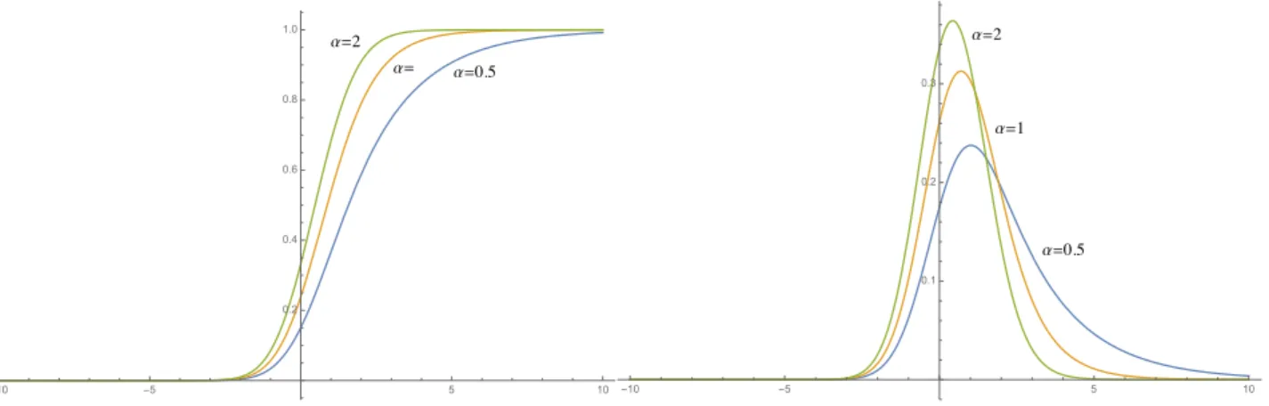
α=��� α= α=� -10 -5 5 10 0.2 0.4 0.6 0.8 1.0 α=��� α=� α=� -10 -5 5 10 0.1 0.2 0.3
Figure 1: CDF and PDF of M-skewed normal distribution for α= 0.5, 1, 2.
Proof. Note that
lim y→−∞M(y;α, w) =−we α2/2 lim y→−∞ Φ(y−α) eαy =−we α2/2 lim a→−∞ ϕ(y−α) αeαy = weα2/2 α√2π y→−∞lim e −12[y2+α2] = 0 lim y→+∞M(y;α, w) = limy→+∞Φ(y)−we α2/2 lim y→+∞ Φ(y−α) eαy = 1 Moreover,
m(y;α, w) = M′(y;α, w) =ϕ(y) +αwe−αy+α2/2Φ(y−α)−we−αy+α2/2ϕ(y−α) = =ϕ(y)+wαe−αy+α2/2Φ(y−α)−√w
2πe
−αy+α2/2
e−12(y−α)2 =wαe−αyΦ(y−α) + (1−w)ϕ(y)>0.
In other words, the functions M(y;α, w) and m(y;α, w) may be considered as CDF and, respectively, PDF of some probability distribution parametrized by α >0, 0 ≤w ≤ 1. More-over, if w = 0 we obtain a normal distribution function. In general case this distribution is characterized the following characteristics :
• Mean value is equal to w
α • Variance is equal to1 + (2−w)w α2 • Skewness is equal to 2w(w 2−3w+ 3) ((2−w)w+α2)3/2 >0 • Kurtosis is equal to 3 + 6w(2−w)(w 2−2w+ 2)
(α2+ (2−w)w)2 , or, equivalently, excess is equal to
6w(2−w)(w2−2w+ 2)
(α2+ (2−w)w)2 >0
As result, the considered distribution is a positive skewed and leptokurtic.
Three examples of their plots for various values of parameter α and w= 1are presented on the Figure 1. We will call it theM-skewed normal distribution.
Vasicek-Merton Distribution of Loss
Using the newly introduced distribution function M(y;w, α) with substituted
y = Φ −1(p)−√ρz √ 1−ρ , α= p 1−ρσ√T
we can represent the formula (7) as follows
pV M(z) =M Φ−1(p)−√ρz √ 1−ρ , w . (8)
Obviously, functionpV M(z)increases with respect topand decreases with respect toz, because CDFM(y, w)strictly increases with respect toy. As result, the conditional loss functionpV M(z)
positively correlated with the conditional share of defaultspV(z)for any given market shockz. Indeed, pV = Φ Φ−1(p)−√ρz √ 1−ρ ⇐⇒ z = Φ− 1(p)−√1−ρΦ−1(pV) √ρ , which implies pV M =M Φ−1(pV), w ,
while both M and Φ−1 are strictly increasing functions.
Lemma 1 implies that there exists inverse function M−1(x), which is well-defined for all
x ∈ (0,1). Then the inverse function f(x) = p−V M1 for x ∈ (0,1) is well-defined as unique solution of equation pV M(z) = x, which implies
Φ−1(p)−√ρz √ 1−ρ =M −1(x) ⇐⇒ z =f(x) = Φ− 1(p) √ρ − r 1−ρ ρ M −1(x) (9) Hence FV M(x) =P(L < x) = P(z > f(x)) = Φ(−f(x)) = =Φ r 1−ρ ρ M −1(x) − Φ− 1(p) √ρ (10)
is the Vasicek-Merton Loss distribution function.
Lemma 2. Given w < w′, the inequality FV M(x, w′) < FV M(x, w) holds for all x ∈ (0,1). In
particular, Vasicek loss distribution FV(x) = FV M(x,0) < FV M(x, w) for all positive recovery
rates w >0.
Proof. Direct comparison of (4) and (7) shows that pV M(z, w′) > pV M(z, w) for all z, while
pV M(z) is strictly decreases functions, therefore p−V M1 (x, w′) > p−1
V M(x, w). CDF Φ is strictly
increasing, hence FV M(x, w′) = Φ(−pV M−1 (x, w′))<Φ(−p−
1
V M(x, w)) =FV M(x).
Figure 2 shows three example of CDFs for the recovery rate valuesw= 1 (solid curve),w= 0.5(dashed curve) and dotted curve of the Vasicek loss distribution FV(x), which corresponds tow = 0.
Now consider the corresponding PDF fV M(x) = FV M′ (x). The case w = 0 corresponds to
the well-studied pure Vasicek distribution, thus in what follows we will assume that w >0.
Lemma 3. Let w >0, then probability density function satisfies the following conditions:
fV M(0) =
(
0 ρ <1/2
+∞ ρ >1/2, fV M(1) = 0.
In case of ρ = 1/2, fV M(0) = 0 for p > 1/2 and fV M(0) = +∞ for p < 1/2. If ρ = 1/2,
�=� �=��� �=� 0.2 0.4 0.6 0.8 1.0 0.2 0.4 0.6 0.8 1.0
Figure 2: Vasicek-Merton CDFs for recovery rate values w= 1,w= 0.5,w= 0
Proof. Calculating the derivative directly, we obtain
fV M(x) = (−f′(x))ϕ(−f(x)) =−f
′(x)
√ 2πe
−12f2(x) (11)
where f(x) is determined by (9). The derivative of an inverse function
f′(x) =− r 1−ρ ρ d dxM −1(x) = − r 1−ρ ρ 1 m(f(x)) = =− r 1−ρ ρ e−√1−ρσ√T y(f(x)) wp (1−ρ)T σΦ(y(f(x))−p (1−ρ)T σ/2) + (1−w)ϕ(y(f(x))−p (1−ρ)T σ/2), (12) where y(z) = Φ −1(p)−√ρz √ 1−ρ − p (1−ρ)T σ 2
Combining (11) and (12) we obtain
fV M(x) = r 1−ρ 2πρ e Φ−1(p)√T σ−(1−ρ)T σ2 2 G(f(x)) H(f(x)), where G(z) =e−12z2− √ ρT σz H(z) = wp(1−ρ)T σΦ Φ−1(p)−√ρz √ 1−ρ − p (1−ρ)T σ + +(1−w)ϕ Φ−1(p)−√ρf(x) √ 1−ρ − p (1−ρ)T σ
Note thatf(1) =−∞, therefore, G(f(1)) = 0, H(f(1)) =wp(1−ρ)T σ >0 if w >0, then
fV M(1) = G(f(1))
Given f(0) = +∞, we have G(f(0)) = 0, H(f(0)) = 0, therefore using a L’Hospital rule, we obtain fV M(0) = r 1−ρ 2πρ e Φ−1(p)σ√T−(1−ρ)σ 2 T 2 lim x→0 G(f(x)) H(f(x)) = r 1−ρ 2πρ e Φ−1(p)σ√T−(1−ρ)σ 2 T 2 lim x→0 G′(f(x)) H′(f(x)). Moreover, G′(f(x)) H′(f(x)) = s 2π(1−ρ) ρ e 1 2 Φ−1(p) √1 −ρ − √ (1−ρ)T σ 2 × × f(x) +√ρσ√Te−12f(x)2 1− 2ρ 1−ρ− Φ−1(p)√ρ 1−ρ f(x) wσ√T + (1−w)q1−ρρf(x)− Φ−1(p) √1 −ρ + p (1−ρ)T σ
First consider the special case w= 1, then
lim x→0 G′(f(x)) H′(f(x)) = 1 σT s 2π(1−ρ) ρ e 1 2 Φ−1(p) √1 −ρ− √ (1−ρ)T σ 2 lim x→0 f(x) +pρT σe−12f(x)2 1− 2ρ 1−ρ− Φ−1(p)√ρ 1−ρ f(x)
If ρ < 1/2 ⇐⇒ 11−−2ρρ > 0, then fV M(0) = 0, while ρ > 1/2 implies fV M(0) = +∞. If
ρ = 1/2, then result depends on sign of Φ−1(p), namely, p ≤ 1/2 ⇐⇒ Φ−1(p) ≤ 0 implies
fV M(0) = +∞, whilep > 1/2 ⇐⇒ Φ−1(p)>0implies fV M(0) = 0.
Now assume w <1, then
lim x→0 G′(f(x)) H′(f(x)) = √ 2π(1−ρ) ρ(1−w) e 1 2 Φ−1(p) √ 1−ρ − √ (1−ρ)T σ 2 lim x→0e −12f(x)2 1− 2ρ 1−ρ− Φ−1(p)√ρ 1−ρ f(x)
which implies the rest statements of the Lemma.
One can see that ifρ <1/2the shapes of VasicekfV(x;p, ρ)and Vasicek-MertonfV M(x;w, p, ρ, σ, T)
functions look similar, though, the densityfV M is more “concentrated”, as it is shown in Figure 3.
On the other hand, it is well-known that in case of ρ > 1/2 the Vasicek density of loss became U-shaped getting the second mode at x = 1, while the Vasicek-Merton density is always unimodal. The Figure 4 shows the behavior of fV(x) and fV M(x) with w = 0.5 for
ρ= 0.65 in neighborhood ofx= 1. To the difference more visible we use the logarithmic scale for y-axis. The second mode at x = 1 is obvious for the Vasicek density, as well as for its logarithm, while the Vasicek-Merton distribution the only mode is at x= 0.
3
Endogenous LGD in Vasicek-Merton Model vs Basel
Ad-justments
The basic assumption that the credit portfolio is homogeneous, i.e., for all firms the probability of default p and volatility σ are the same, implies that the Loss Given Default
LGD= 1
pE(1−wa(T)|a(T)<1).
Given
�=��� �=� �=� 0.2 0.4 0.6 0.8 1.0 5 10 15
Figure 3: PDFs of Vasicek-Merton loss distributions for ρ = 0.25 and w = 1 (solid curve),
w= 0.5 (dashed curve), w= 0 (dotted curve).
a) ���(��) 0.2 0.4 0.6 0.8 1.0 5 10 b) ���(���) 0.2 0.4 0.6 0.8 1.0 -400 -300 -200 -100
Figure 4: Density plots in logarithm scale of Vasicek (a) and Vasicek-Merton (b) loss distribu-tion for ρ= 0.65 .
the condition a(T)<1is equivalent to lna(0) + (r−σ2/2)T +σ√T ε <0 ⇐⇒ ε <−lna(0) + (r−σ 2/2)T σ√T =−d− which implies LGD = 1 p Z −d− −∞ 1·ϕ(t)dt−wa(0)e(r−σ2/2)T Z −d− −∞ eσ√T t√1 2πe −1 2t2dt = =1 p Φ(−d−)−wa(0)erT Z −d− −∞ 1 √ 2πe −12(t−σ √ T)2 d(t−σ√T) = =1 p " Φ(−d−)−wa(0)erT Z −d−−σ √ T −∞ 1 √ 2πe −12z2dz # = =1 p Φ(−d−)−wa(0)erTΦ(−d+) , where d+=d−+σ √ T = lna(0) + (r+σ 2/2)T σ√T . Given p= Φ(−d−) ⇐⇒ d+ =σ √ T −Φ−1(p) and a(0) =e−[√T σΦ−1(p)+(r−σ2/2)T]
we obtain the following identity
LGD(p) = 1− w pe −σ√TΦ−1(p)+σ2T 2 Φ Φ−1(p)−σ√T. Let Ψ(x)≡ Φ(x) ϕ(x),
then the previous formula for LGD may be rewritten as
LGD(p) = 1−wΨ
Φ−1(p)−σ√T
Ψ (Φ−1(p)) (13)
In case of w= 0we obtain the pure Vasicek model withLGD(p)≡1. Moreover, in working paper [Altman et al.] this formula (in terms ofd±) was obtained for the case of w= 1.
Assume that w >0, then the following statement holds.
Proposition 1. LGD(0) = 1−w < 1, LGD(1) = 1 and LGD increases with respect p,σ and
T.
Proof. An identity LGD(1) = 1 is obvious. Let t = Φ−1(p), s = σ√T, then to prove that
LGD(0) = 1−w it is sufficient to show lim t→−∞ e−stΦ (t−s) Φ(t) =e −s2/2 . Note that lim t→−∞e −stΦ (t −s) = lim t→−∞ Φ (t−s) est = limt→−∞ ϕ(t−s) sest = 1 √ 2πt→−∞lim e −12(t2+s2) = 0,
therefore, applying the L’Hospital rule we obtain lim t→−∞ e−stΦ (t−s) Φ(t) = limt→−∞ −se−stΦ (t−s) +e−stϕ(t−s) ϕ(t) =e −1 2s2 −s lim t→−∞ e−stΦ (t−s) ϕ(t) = =e−12s2 −s√2π lim t→−∞ Φ (t−s) e−12t2+st =e−12s2 −s lim t→−∞ e−12t2+st− 1 2s2 (s−t)e−12t2+st =e−12s2
To justify increasing with respect to σ and T, it is sufficient to prove that LGD increases with respect to let s=σ√T. Indeed,
∂ ∂sLGD = w pe −sΦ−1(p)+s2/2 ϕ(Φ−1(p)−s)−(s−Φ−1(p))Φ Φ−1(p)−s .
Let x = s−Φ−1(p), then for x ≤ 0 an inequality ϕ(−x)−xΦ(−x) > 0 is obvious, while for
x > 0 an inequality ϕ(−x) = ϕ(x) > xΦ (−x) is well-known upper-tail property for standard normal distribution.
Finally, an increasing of the function LGD(p) with respect to pis equivalent to inequality
∂ ∂t e−stΦ (t−s) Φ(t) <0 Indeed, ∂ ∂t e−stΦ (t−s) Φ(t) =e−st−sΦ (t−s) Φ(t) +ϕ(t−s)Φ(t)−Φ (t−s)ϕ(t) Φ(t)2 Let G(t) = −sΦ (t−s) Φ(t) +ϕ(t−s)Φ(t)−Φ (t−s)ϕ(t),
then limt→−∞G(t) = 0 and
G′(t) = (t−s)Φ (t−s)ϕ(t)−tϕ(t−s)Φ(t).
It is obvious, that G′(t) < 0 for all t ≤ s, assume t > s > 0, then ϕ(t) < ϕ(t −s) and
(tΦ(t))′ >0, hence
G′(t)< ϕ(t−s) [(t−s)Φ (t−s)−tΦ(t)]<0,
which implies G(t)<0 for all t. In turn, this means that
∂ ∂t e−stΦ (t−s) Φ(t) <0 ⇐⇒ d dpLGD > 0.
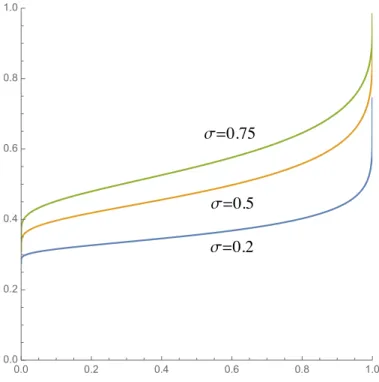
The Figure 3 illustrates the results of Proposition 1 showing three plots of the function
LGD(p)for T = 1 and three values of σ = 0.2, 0.5, 0.75. where λB(p, T) = lgd· 1 + (T −2.5)·b(p) 1−1.5·b(p) =lgd· 1 + (T −1)· b(p) 1−1.5·b(p) b(p) = (0.11852−0.05478 ln(p))2, M−1(x)is inverse function to M(y) = Φ(y)−we−αy+α2/2Φ(y−α), Ψ(x) = Φ(x) ϕ(x).
It worth to mention that CDF formula FB(x) implies that the corresponding PDF fB(x) = F′
B(x) satisfies fB(x) ≡ 0 for all x > λB(p, T), in particular, fB(1) = 0 even if ρ > 1/2. This
means that the AIRB-adjusted Vasicek density of loss, likewise the Vasicek-Merton density and unlike the vanilla Vasicek PDF, has no second mode at x= 1 in case of ρ >1/2.
σ=��� σ=��� σ=���� 0.0 0.2 0.4 0.6 0.8 1.0 0.0 0.2 0.4 0.6 0.8 1.0
Figure 5: How LGD depends on Probability of Default
Distribution CDF LGD Vasicek FV(x) = Φ√1−ρΦ−1(x)−Φ−1(p) √ρ 1 AIRB FB(x) = Φ √ 1−ρΦ−1 x λB(p,T) −Φ−1(p) √ρ , x < λB(p, T) 1, o/w λB(p, T) Vasicek-Merton FV M(x) = Φ√1−ρM−1(x)−Φ−1(p) √ρ 1−wΨ(Φ−1(p)−σ √ T) Ψ(Φ−1(p)) <1
Comparison with Basel adjustments
To compare the Basel and Vasicek-Merton approaches, note that the Basel adjustment coeffi-cient λB(p, T) = lgd· 1 + (T −2.5)·b(p) 1−1.5·b(p) =lgd· 1 + (T −1)· b(p) 1−1.5·b(p) b(p) = (0.11852−0.05478 ln(p))2
satisfies λB(p,1) = lgd for all p, i.e., the exogenous parameter lgd is considered as a loss given default in case of the maturity T = 1. This means that λB(p, T) may be interpreted as an expansion of the one-period lgd on an arbitrary maturity T, which also depends on the probability of default p. On the other hand, the generalized Vasicek-Merton model implies the following form of general Loss Given Default function
λV M(p, T) = 1−w ΨΦ−1(p)−σ√T Ψ(Φ−1(p))) , where Ψ(x)≡ Φ(x) ϕ(x),
Note that, generally speaking, λB(p, T) and λV M(p, T) are hardly comparable, because
λB(p, T)depends on exogenous constantLGD, while λV M(p, T)is based on another exogenous
constant w. To make them more close, assume that the following identity holds
lgd=λV M(p,1) = 1−w
Ψ (Φ−1(p)−σ)
Ψ(Φ−1(p))) .
Given that, let’s compare the distributions of loss, generated by Basel adjustments of loss and by Vasicek-Merton model. The Vasicek-Merton cumulative distribution function
FV M(x) = Φ r 1−ρ ρ M −1(x) − Φ− 1(p) √ρ
was derived in previous section, while the Basel CDF is obviously equal to
FB(x) = FV x λB(p, T) = Φ r 1−ρ ρ Φ −1 x λB(p, T) − Φ− 1(p) √ρ
It is worth to mention, that unlike the vanilla Vasicek loss distribution, the Basel PDF
fB(x) = F′
B(x) is not U-shaped in case ρ > 1/2. Indeed, if λB(p, T) < 1 then λB(xp,T) ≥ 1 for
all x ∈(λB(p, T),1], which implies FB(x) = 1 and fB(x) = 0 in some neighborhood of x = 1. Note that for the Vasicek-Merton loss distribution the PDFfV M(1) = 0 due to Lemma 3.
The Figure 6 plots the corresponding PDF for the Basel distribution (solid curve), Vasicek-Merton distribution (dotted curve) and non-adjusted Vasicek distribution (dashed curve) for
p= 0.05,σ = 0.2, w= 0.5, T = 1; the correspondingρ is equal to
ρ= 0.121−e− 50p 1−e−50 + 0.24· 1−1−e− 50p 1−e−50 ≈0.13.
The variation of model parameters results in more different curves. Figure 7 presents,ceteris
paribus, the cases T = 2 and T = 3. Hereafter we will skip a plotting of the vanilla Vasicek
graphs, filling the space between Vasicek-Merton and Basel curves for more visibility. As one can see, the longer is a maturityT, the more is difference between curves. This means that the linear with respect toT maturity adjustment does not fit well the Vasicek-Merton distribution.
��(�)≈���(�) ��(�) 0.05 0.10 0.15 0.20 0.25 0.30 5 10 15 20 25 30
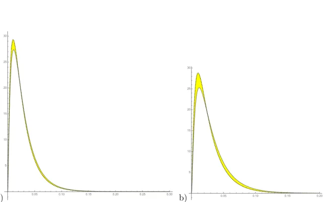
Figure 6: Density functions for Vasicek, AIRB-adjusted Vasicek and Vasicek-Merton distribu-tions, p= 0.05,σ = 0.2, w= 0.5, T = 1 a) 0.05 0.10 0.15 0.20 0.25 0.30 5 10 15 20 25 30 b) 0.05 0.10 0.15 0.20 5 10 15 20 25 30
Figure 7: Density functions for Vasicek, AIRB-adjusted Vasicek and Vasicek-Merton distribu-tions, p= 0.05,σ = 0.2, w= 0.5, T = 2 (a) andT = 3 (b).
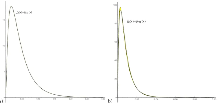
a) ��(�)≈���(�) 0.05 0.10 0.15 0.20 0.25 0.30 5 10 15 b) ��(�)≈���(�) 0.02 0.04 0.06 0.08 0.10 20 40 60 80 100
Figure 8: Density functions for Vasicek, AIRB-adjusted Vasicek and Vasicek-Merton distribu-tions, p= 0.05,σ = 0.2, T = 1, w= 0.1 (a) andw= 0.9 (b).
Other parameters variation
Figures 6 and 7 show that variation of maturity T results in difference between distributions of loss in Basel and Vasicek-Merton approaches. On the other hand, in case of T = 1 variation of of the parameters has no significant consequence. Figure 8 shows three example forw= 0.1, 0.9
, while p= 0.05, σ = 0.2,T = 1.
Figure 9 variates the probability of p= 0.01, 0.2, while,σ = 0.2, w= 0.5, T = 1.
Finally, the variation of σ= 0.1, 0.5, while p= 0.05,w= 0.5,T = 1 is presented on Figure 10. As before, only the unusually large value of parameter σ = 0.5 shows the visible difference between Basel and Vasicek-Merton.
To measure a difference between distributions consider the threshold values of loss at the confidence level 0.999 required by Basel, i.e., solutions of equationF(x) = 0.999 for the corre-sponding CDFs. The vanilla Vasicek CDF provides the well-known solution
x∗V = Φ Φ−1(p) +√ρΦ−1(0.999) √ 1−ρ ,
the Basel adjustments transforms the previous formula into
x∗B =λB(p, T)·Φ Φ−1(p) +√ρΦ−1(0.999) √ 1−ρ ,
while the Vasicek-Merton distribution determines
x∗V M =M Φ−1(p) +√ρΦ−1(0.999) √ 1−ρ , where M(y) = Φ(y)−w·e−√1−ρσ√T y+(1−ρ)σ2T /2Φ(y−p1−ρσ√T).
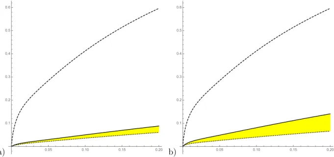
The Figure 11 presents the three plots of x∗
V (dashed curve),x∗B (dotted curve) and x∗V M (solid
curve) considered as functions of the default probability p. The other parameters are set as follows: w= 1, σ= 0.2, T = 1, the correlation ρ is determined using the Basel procedure as
ρ= 0.121−e− 50p 1−e−50 + 0.24· 1−1−e− 50p 1−e−50
a) ��(�)≈���(�) 0.01 0.02 0.03 0.04 50 100 150 200 250 300 b) ��(�)≈���(�) 0.1 0.2 0.3 0.4 2 4 6 8
Figure 9: Density functions for Vasicek, AIRB-adjusted Vasicek and Vasicek-Merton distribu-tions, σ = 0.2,T = 1, w= 0.5, p= 0.01 (a) andp= 0.2 (b).
a) ��(�)≈���(�) 0.1 0.2 0.3 0.4 5 10 15 20 25 30 b) ��(�)≈���(�) 0.1 0.2 0.3 0.4 5 10 15 20 25
Figure 10: Density functions for Vasicek, AIRB-adjusted Vasicek and Vasicek-Merton distribu-tions, T = 1, w= 0.5, p= 0.05, σ = 0.1 (a) andσ = 0.5.
a) 0.05 0.10 0.15 0.20 0.1 0.2 0.3 0.4 0.5 0.6 b) 0.05 0.10 0.15 0.20 0.1 0.2 0.3 0.4 0.5 0.6
Figure 11: Threshold plots for Vasicek, Vasicek-Merton and Basel distributions of loss at con-fidence level 0.999 for w= 1,σ = 0.2, T = 1 (a) andT = 3 (b).
As one can see, Basel and Vasicek-Merton thresholds are very close to each other for T = 1, while in case T = 3 thresholds differ significantly. Anyway, this difference is less substantial in comparison with non-adjusted Vasicek case.
Conjecture. The Basel adjustment of Vasicek loss distribution is actually based on an
approx-imation of the endogenous Loss Given Default (13) in the neighborhood of T = 1.
4
Concluding Remarks
The Vasicek-Merton loss distribution, that is introduced and studied in this paper, may help in solution of the “mystery of AIRB adjustments.” Due to the authors’ opinion, the theoreti-cal basis behind these adjustments is exactly the Vasicek-Merton distribution approximated in neighborhood of the typical values of parameters. There is an almost ideal coincidence of two distribution where the first one was derived from the pure theoretical basis while the numerical coefficients of the second one are obviously obtained by approximation and/or regression on some date, which cannot be simply an accident. We believe that the Vasicek-Merton distri-bution is a key to the “black box” of AIRB adjustment. On the other hand, in long-run, for maturity T >> 1, the difference between these two distribution become significant, thus an AIRB adjustment of Vasicek distribution cannot be considered as a good approximation of the Vasicek-Merton distribution. This arises the second implication of the presented paper (pro-vided that we accept the hypothesis on the theoretical key to AIRB adjustments): it should use the exact Vasicek-Merton formula instead of its approximation. This does note arises too large computational problem, because, from the technical point of view, the formula of the Vasicek-Merton distribution involves a “skewed” normal distribution function instead of the standard normal one.
References
[1] Altman, E., Brady, B., Resti, A., and Sironi, A., (2005), The Link between Default and Recovery Rates: Theory, Empirical Evidence and Implications. J. of Business. 78(6), 2203– 2228.
[2] BIS, An Explanatory Note on the Basel II IRB Risk Weight Functions, July 2005, https://www.bis.org/bcbs/irbriskweight.pdf
[3] Black, F., Scholes, M. (1973), The pricing of options and corporate liabilities. J. Polit. Econ. 81:637–54
[4] Frye, J. (2013), Loss given default as a function of the default rate, Federal Reserve Bank of Chicago, 1 – 15.
[5] Kupiec, P. H. (2009), How Well Does the Vasicek-Basel Airb Model Fit the Data? Evidence from a Long Time Series of Corporate Credit Rating Data, FDIC Working Paper Series [6] Merton, R.C., (1974), On the pricing of corporate debt: the risk structure of interest rates.
J. Finance, 29:449–70
[7] Vasicek O., (1987), Probability of Loss on Loan Portfolio, KMV Corporation