Hybrid algorithm for missing data imputation and its application to electrical data loggers

(1)

Article

A Hybrid Algorithm for Missing Data Imputation and

Its Application to Electrical Data Loggers

Concepción Crespo Turrado1, Fernando Sánchez Lasheras2,*, José Luis Calvo-Rollé3, Andrés-José Piñón-Pazos3, Manuel G. Melero4and Francisco Javier de Cos Juez5

1 _{Maintenance Department, University of Oviedo, San Francisco 3, Oviedo 33007, Spain; [email protected]} 2 _{Department of Construction and Manufacturing Engineering, University of Oviedo, Campus de Viesques,}

Gijón 33204, Spain

3 _{Departamento de Ingeniería Industrial, University of A Coruña, A Coruña 15405, Spain;}

[email protected] (J.L.C.-R.), [email protected] (A.-J.P.-P.)

4 _{Electrical Engineering Department, University of Oviedo, Campus de Viesques, Gijón 33204, Spain;}

[email protected]

5 _{Prospecting and Exploitation of Mines Department, University of Oviedo, Oviedo 33004, Spain;}

[email protected]

* Correspondence: [email protected]; Tel.: +34-984-833-135; Fax: +34-985-182-433

Academic Editor: Kemal Akkaya

Received: 13 July 2016; Accepted: 7 September 2016; Published: 10 September 2016

Abstract: The storage of data is a key process in the study of electrical power networks related to the search for harmonics and the finding of a lack of balance among phases. The presence of missing data of any of the main electrical variables (phase-to-neutral voltage, phase-to-phase voltage, current in each phase and power factor) affects any time series study in a negative way that has to be addressed. When this occurs, missing data imputation algorithms are required. These algorithms are able to substitute the data that are missing for estimated values. This research presents a new algorithm for the missing data imputation method based on Self-Organized Maps Neural Networks and Mahalanobis distances and compares it not only with a well-known technique called Multivariate Imputation by Chained Equations (MICE) but also with an algorithm previously proposed by the authors called Adaptive Assignation Algorithm (AAA). The results obtained demonstrate how the proposed method outperforms both algorithms.

Keywords: missing data imputation; multivariate imputation by chained equations (MICE);

Mahalanobis distances; Self-Organized Maps Neural Networks (SOM); Adaptive Assignation Algorithm (AAA); Multivariate Adaptive Regression Splines (MARS); quality of electric supply; voltage; current; power factor

1. Introduction

Currently, the importance of problems due to harmonics in electric networks is growing. This fact is due to the increase in the amount of non-linear loads. The two main problems related to harmonics are the overheating of conductors due to the skin effect and the activation of automatic breakers, which produce problems for supply continuity. Additionally, distortion of the voltage waveform may cause the malfunction of some devices. The monitoring of harmonics in real time is required to control them.

Another common problem in electrical networks is the imbalance between phases. This is usually caused by a bad load distribution between phases and provokes a high current return displayed by the neutral, as it has to compensate for the gap existing at the centre of the scheme vectors.

Electricity quality is an important issue that is present in the following variables: voltage, current, frequency anomalies, etc. The quality affects all devices connected to the power network, causing failure of the systems or disability [1]. Currently, an electric system is analyzed in terms of efficiency, Sensors2016,16, 1467; doi:10.3390/s16091467 www.mdpi.com/journal/sensors

(2)

stability and optimization to obtain better quality of the system [2]. With the aim of reducing the issues and improving electricity quality, science and technology are evolving to mitigate problems and overcome the problems mentioned above [3].

Different studies in this field have been performed: for instance, a novel power quality deviation parameter based on principal curves is presented in [4]. In [5], a review of the signal processing and intelligent techniques and methods employed in the self-classification of the events of power quality and the influence of noise on the recognition and classification of perturbations has been made. [6] describes a device capable of labelling, recognizing, and quantifying energy and power quality perturbation. An intelligent device for high-resolution frequency measuring that agrees with the common indicator standards is shown in [7]; it is used for electricity quality monitoring and control. Furthermore, [8] exposes a communication infrastructure created to obtain consistent data delivery at low cost, with the aim to prevent the difficulties of the power quality monitoring service.

Monitoring the main electrical variables in electric systems in some buildings might be interesting. Therefore, monitoring is useful for the control with the objective of balancing the loads of a building, thus reducing the consumption of the electric energy of the building by decreasing the remaining consumption (during non-working hours). The analysis of the electric system in buildings is useful for determining the optimized rates. Furthermore, it is also useful for the analysis of supply issues that can affect the different loads, which are caused by a lack of balance or harmonics, analysis of the energy quality and preventing incidents as a result of poor signal quality. Finally, the analysis of the building operation and its efficiency study might be of interest when accounting for the dependency of the people who use it, area in use, installed power, etc.

During the data-collection process, it is likely that a small amount of the information retrieved may be lost. In these cases, missing data imputation algorithms must be applied because the substitution of missing data with zeros is not acceptable. The present research evaluates a new imputation method that is able to predict the value of any missing data in the sensor devices that are used in this research for the recording of electrical variables. The new algorithm is based on Self-Organized Maps Neural Networks and Mahalanobis distances and hybridizes them with the algorithm called the Adaptive Assignation Algorithm (AAA). The results obtained are benchmarked with those given by the AAA and multivariate imputation by chained equations (MICE) [9].

The rest of the paper is arranged as follows: Section2describes the measurement equipment and the database, Section3details the proposed algorithm and how its performance is measured and compared. Section4presents the results obtained and its comparison with other algorithms. Finally, the conclusions are drawn in Section5.

2. Materials and Methods

2.1. Measurement Equipment

In this section, the specific power quality measurement devices that are employed in this work are described (Figure1). The next measurements are common to all them, namely: Energy Output or Input (ENERGY), Reactive Energy Output or Input (R-ENERGY), Apparent Energy (A-ENERGY), Power Factor (P-F), Power Output or Input (POW), Reactive Power (R-POW), Apparent Power (A-POW), Voltage from Line to Line (VLL), Voltage from Line to Neutral (VLN), Current by line (I), and Frequency (FQ). The accuracy of each electrical measurement for all devices used is shown in Table1. Note that all indicated percentage values refer to the obtained percentage.

(3)

Sensors2016,16, 1467 3 of 13 Table 1. Device precision. POW: power, R-POW: reactive power, A-POW: active power, A-ENERGY: active energy, VLN: voltage line to neuter, VLL: voltage line to line, I: current, PF: power factor, FQ: frequency.

Variable Units MP200 NEXUS 1252 SK-200 SK-100 (%) 200 mili Seg (%) 1 s (%) (%) (%)

POW W 0.5 0.1 0.06 0.2 0.2

ENERGY W·h 0.5 N/A 0.04 0.2 0.2

R-POW VARs 1.0 0.1 0.08 0.2 0.2

R-ENERGY VAR·h 1.0 N/A 0.08 0.2 0.2

A-POW VA 1.0 0.1 0.1 0.2 0.2

A-ENERGY VA·h 1.0 N/A 0.08 0.2 0.2

VLN V/KV 0.3 0.1 0.05 0.1 0.1 VLL V/KV 0.5 0.1 0.05 0.2 0.1 I A/KA 0.3 0.1 0.025 0.1 0.1 PF 0.5 to 1 1.0 0.1 0.08 0.2 0.2 FQ (*) Hz ±10−2 _{* 3.10}−2 _{* 1.10}−2 _{* ±3.10}−2 _{* 1.10}−2 _* * Accuracy in Hz.

Figure 1. Equipment (SK-100/200 on the left, Nexus1250 on the right top and MP200 on the right bottom; source: Electro Industries/GaugeTech, Westbury, New York—USA) [10].

2.2. The Data Description

In this paper, the next dataset, which includes measurements of variables from an electrical power supply of an edifice, has been used.

 Three variables of each phase current

 Three variables of voltage from phase to phase

 Three variables of voltage from phase to neutral

 Average power factor

Between the 27 November 2014 at 18:45 and the 31 May 2015 at 23:45, the data set was logged, with an interval of 15 min.

A building called Severo Ochoa, in honour of the Novel Prize winner, was used in this work for the dataset. The University of Oviedo (Spain) is the owner of this building, which has a total area of

Figure 1. Equipment (SK-100/200 on the left, Nexus1250 on the right top and MP200 on the right bottom; source: Electro Industries/GaugeTech, Westbury, New York—USA) [10].

Table 1.Device precision. POW: power, R-POW: reactive power, A-POW: active power, A-ENERGY: active energy, VLN: voltage line to neuter, VLL: voltage line to line, I: current, PF: power factor, FQ: frequency.

Variable Units MP200 NEXUS 1252 SK-200 SK-100

(%) 200 mili Seg (%) 1 s (%) (%) (%)

POW W 0.5 0.1 0.06 0.2 0.2 ENERGY W·h 0.5 N/A 0.04 0.2 0.2 R-POW VARs 1.0 0.1 0.08 0.2 0.2 R-ENERGY VAR·h 1.0 N/A 0.08 0.2 0.2 A-POW VA 1.0 0.1 0.1 0.2 0.2 A-ENERGY VA·h 1.0 N/A 0.08 0.2 0.2 VLN V/KV 0.3 0.1 0.05 0.1 0.1 VLL V/KV 0.5 0.1 0.05 0.2 0.1 I A/KA 0.3 0.1 0.025 0.1 0.1 PF 0.5 to 1 1.0 0.1 0.08 0.2 0.2 FQ (*) Hz ±10−2* 3.10−2* 1.10−2* ±3.10−2* 1.10−2* * Accuracy in Hz.

All mentioned measurements can be performed by the four devices used in the present work. The four devices have additional features. Shark 100, Shark 200 and Shark MP200 incorporate V-Switch technology, which allows the operator to add new functions to the devices using programming commands at any time after its installation. In the case of the Nexus 1252 device, it is possible to add isolated input/output modules and software options for additional functions. All of them have communication capabilities (some optional) as Modbus or DNP 3.0 (Distributed Network Protocol) protocols by an RS485 port, 10/100BaseT Ethernet capabilities or IrDA port. A deep analysis of features of each device is made in [10].

2.2. The Data Description

In this paper, the next dataset, which includes measurements of variables from an electrical power supply of an edifice, has been used.

(4)

• Three variables of each phase current

• Three variables of voltage from phase to phase • Three variables of voltage from phase to neutral • Average power factor

Between the 27 November 2014 at 18:45 and the 31 May 2015 at 23:45, the data set was logged, with an interval of 15 min.

A building called Severo Ochoa, in honour of the Novel Prize winner, was used in this work for the dataset. The University of Oviedo (Spain) is the owner of this building, which has a total area of 8.150 m2, distributed over two basement levels and five floors; a total of 78 employees work in it. The ITS (Information Technology Services) of the University of Oviedo are also located in this edifice. The equipment of the ITS is distributed across server rooms and scientific laboratories. This equipment has to be supplied by a good quality power network at all times. The laboratory equipment mentioned above includes electron microscopes, NMR spectrometers, X-ray diffractometers, etc. The energy consumption is 190.572 KWh per day, on average. The data set detailed here was already employed by the authors in previous research [9].

The equipment mentioned above, and the building services, incorporate devices such as UPS (Uninterruptible Power Supply), VSD (Variable Speed Drive) and inductive and capacitive loads in switching mode. These electronic circuits are nonlinear loads, and all of them can create harmonic distortion in the power line. The harmonic distortion in the distribution system is caused by the harmonic currents flowing in the electronic loads.

3. Methodology

The data set employed in this research has a total of 17,763 samples that correspond to the period of time referred to in the description of the data. A process of random data deletion was performed using this data set.

The new algorithm presented in this paper hybridizes the Self-Organized Maps Neural Networks methodology with the Mahalanobis distances. The hybrid method obtained is combined with an algorithm already presented in this journal by the authors, called AAA [9], based on Multivariate Adaptive Regression Splines. The proposed methodology is new and its performance is even better than the one referenced and presented in a previous paper when applied to the same database. This method is considered a hybrid method because it combines well-known pattern recognition and machine learning methodologies in a hybrid model that is able to impute missing data [11,12].

The performance of the proposed new methodology, in comparison with AAA and MICE, has been evaluated using the mean absolute error (MAE) and the root mean square error (RMSE). They are very common metrics in forecasting research [13,14]. The reason why, in the present research, both are employed is their complementarity. The purpose of the MAE is the measurement of the average magnitude of the error in a set of forecasts without considering their direction while the RMSE is employed for its ability to describe uniformly distributed errors [13]. A more detailed explanation including the formulas employed can be found in [9]

Let us assume that we have a dataset formed byc different variablesv1, v2, . . . , vcthat are the columns of a data matrix whose total number of rows isr. The algorithm is applied via the following steps.

3.1. Creation of a New Matrix with Missing Values from the Original Data Set

This step of the algorithm is not required when it is applied to a data set in which missing data are going to be imputed, but it is mandatory in the present research to validate the algorithm by using a complete data set.

Let A be the original matrix (rxc) of r rows and c columns. As a first step and to obtain a matrix with a certain amount of missing data, a proportion of p elements in the matrix is removed. Let B be

(5)

the new (rxc) matrix, with a proportion p of missing elements. The removal is performed completely at random; therefore, the type of imputation that is going to be tested to determine the performance of the algorithm is the one known as missing completely at random (MCAR).

3.2. Creation of the Reduced Matrix

A new matrix in which all the rows with missing data are removed is created. This new matrix is calledBred. Although the number of rowss(s≤r) of this matrix will change depending on the matrix that is going to be imputed, in those cases like the one presented in this algorithm in which the removal of data has been performed completely at random and in a proportion p, the number of remaining rows u will be represented by the following formula:

u=r×(1−p)c, (1)

where:

p: proportion of missing data considered; r: number of rows of the original matrix; c: number of columns of the data matrix; Afterwards theBred_{matrix is normalized.}

3.3. Determination of the Director Vectors by Means of Self-Organized Maps Neural Networks

The Self-Organized Maps (SOM) Neural Network is a type of unsupervised neural-network algorithm whose main application is related to the visualization and interpretation of large dimensional data sets [15].

These types of maps are used to represent all the available observations (data vectors), with an optimized accuracy, by means of a reduced set of models. This is the reason why this technique has been chosen in the present research.

Let N be the dimension of the n director vectors X(t)∈Rn, t = 1, 2, . . . , n, where each sample vector is identified by a label. The two-dimensional output layer of the SOM map contains a rectangular mesh of k = 1, . . . , xdim×ydimnodes. Each one of these nodes is employed as a codebook vector Wk of dimension N. The calculus of the weight vectors is performed by using the following algorithm [16].

For a certain amount of iterations, follow the steps detailed below: 1. Choose one sample vectorX(t)at random;

2. Search for the nearest weight vector Wc:||X−Wc||=minj||X−Wj||; 3. Update the weightsWiby means of the following rule:

Wi(t+1) =Wi(t) +hci(t)·[X(t)−Wi(t)], (2)

wherehci(t)is the neighbour function, which, in the case of the present research and is being very common in the literature [15], is of the Gaussian type:

hci(t) =α(t)·exp _−|| Wc−Wi || 2·σ2₍_t₎ . (3)

Weight of neurons lying in the neighbourhoodhci(t)of the winning neuron is moved closer to X(t). The learning rateα(t)∈[0, 1]decreases monotously as the number of iterations increases,σ(t)

determining that the radius of the neighbourhood also decreases monotonically. After many iterations and the slow reduction ofα(t)andσ(t), the neighbourhood covers only a single node and the map is formed. Please note that those neurons, whose weights are closer in the parameter spaceW, are also closer on the mesh. After this process, the director vectors obtained are denormalized. The number of

(6)

director vectors chosen to create the Self-Organized Map in the case of the present algorithm is related to the number of rows in theBredmatrix. Letube the number of rows in the matrixBred; the total amount of director vectors will be a range of valuesd=e·u/e∈[0.05, 0.8]; the reason for this range of values, empirically found, will be explained in the results sections.

3.4. Finding the Closest Director Vectors by Means of Mahalanobis Distances

The Mahalanobis distance is a well-known, non-Euclidean distance measure based on correlations between variables [17]. These correlations allow for the identification and analysis of different patterns. This measure is a useful way of determining the similarity of an unknown sample set to a known one, and, in the present research, it is used to compare each one of the rows of the data matrix with missing data with all the director vectors. It can be defined by the following formula:

dA(x1,x2) = q

(x1−x2)T·A·(x1−x2), (4) wherex1andx2represent the sets of variables of two different rows of the data matrix, andA ∈Rnxn is a positively semi-definite matrix that represents the inverse of the covariance matrix of class{I}. By means of the eigenvalue decomposition,Acan be decomposed intoA=W·WT.

In the case of the present algorithm, the Mahalanobis distance of each vector row with two or more missing data points to all the director vectors is calculated. Please note that, in order to make this operation possible, all those variables with missing data in the row that come from the data matrix are removed in the director vector. The director vector with the lowest Mahalanobis distance value is selected and those missing variables in this row of the data matrix are filled using the values present in the corresponding row of the director vector.

Finally, the original matrix is reconstructed and the value of the missing data of those rows with only one or two missing data points are imputed by means of the AAA algorithm. As it has already been stated, this algorithm was presented in a previous work [9] published in this journal. The referenced algorithm is based on a multivariate non-parametric technique called Multivariate Adaptive Regression Splines (MARS) [18–21].

4. Results and Discussion

In this section, the results of the Hybrid Adaptive Assignation Algorithm (HAAA) are presented and compared with those of the AAA and MICE. The test was performed using the MCAR methodology, deleting 10%, 15% and 20% of the information. This process was repeated five times. The performances of the three algorithms were compared based on the MAE and RMSE metrics. The results of all the interactions performed are presented. To simplify the comparisons, the results that use the same original MCAR subsets are presented in the same table. The way in which results are presented is the same as the one that was employed in previous research, in which the performance of the AAA algorithm was analysed [9]. Each table also contains the average values of the five replications. Table2

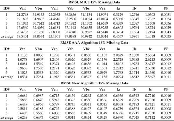
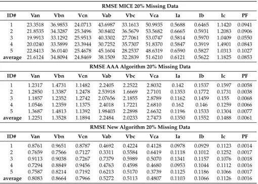
contains the RMSE values of the MICE, AAA and HAAA algorithms when applied to a database with 10% of the data missing. As can be observed in this table, for the variables of voltage, intensity and power factor employed in this research, the RMSE values obtained by the new algorithm are considerably lower than those obtained by using the AAA and MICE methods. In the case of 10% missing data, Table2, the variable in which the RMSE is reduced to a lesser amount receives a 15% reduction, while the average reduction of all variables is 62%. For the case of 15% missing data, Table3, the results are very similar, obtaining at least a reduction of the RMSE of 12% and an average reduction of 46%. Additionally, for the case of 20% missing data, Table4, the results are equivalent, with a minimum 18% reduction of the RMSE value and an average of 48%.

(7)

Table 2.RMSE obtained with 10% missing data using MICE, AAA and the newly proposed algorithm, HAAA. RMSE: root mean square error, MICE: multivariate imputation by chained equations, AAA: adaptive assignation algorithm, HAAA: hybrid adaptive assignation algorithm, Van: voltage line a to neuter, Vbn: voltage line b to neutre, Vcn: voltage line c to neutre, Vab: voltage line a to b, Vbc: voltage line b to c, Vca: voltage line c to a, Ia: current line a, Ib: curren line b, Ic: current line c.

RMSE MICE 10% Missing Data

ID# Van Vbn Vcn Vab Vbc Vca Ia Ib Ic PF

1 20.8398 34.3633 21.9653 30.9830 36.0714 48.0547 0.2653 0.7807 1.6655 0.0030 2 18.7495 31.6307 24.1316 31.0080 37.0614 48.1173 0.7918 0.3262 1.5742 0.0017 3 18.8833 30.4312 24.0313 34.9034 30.8320 47.8822 0.1946 0.1122 1.6727 0.0027 4 17.3260 32.0759 21.2884 31.8996 31.5952 48.7585 0.9634 0.6172 1.8090 0.0030 5 20.0333 34.4660 22.1438 32.1480 32.9437 47.7413 0.7631 0.1324 1.4919 0.0028 average 19.1664 32.5934 22.7121 32.1884 33.7007 48.1108 0.5956 0.3937 1.6427 0.0026

RMSE AAA Algorithm 10% Missing Data

1 1.0583 1.7376 1.1078 1.6251 1.0612 1.8042 0.1318 0.1478 0.1514 0.0030 2 1.0228 1.6687 1.2186 1.4223 2.0596 1.7124 0.1307 0.1749 0.1304 0.0020 3 0.9641 1.5329 1.2044 2.0471 1.9560 1.7213 0.1365 0.1985 0.1172 0.0015 4 0.9328 1.6923 1.1531 1.8030 1.8338 1.8457 0.1845 0.1581 0.1340 0.0021 5 1.0473 1.7783 1.1100 1.7025 1.5521 1.8885 0.1368 0.1374 0.2158 0.0024 average 1.0050 1.6819 1.1588 1.7200 1.6925 1.7944 0.1441 0.1633 0.1498 0.0022

RMSE New Algorithm 10% Missing Data

1 0.6029 0.6657 0.6165 0.0384 0.0218 0.0265 0.0866 0.0632 0.0863 0.0009 2 0.5663 0.6128 0.5283 0.0270 0.0558 0.0503 0.0599 0.0896 0.0687 0.0008 3 0.5789 0.6526 0.5457 0.0690 0.0497 0.0479 0.0768 0.0652 0.0687 0.0061 4 0.5264 0.5965 0.6352 0.0344 0.0383 0.0374 0.0608 0.0624 0.0609 0.0007 5 0.5853 0.5110 0.5568 0.0603 0.0354 0.0316 0.0612 0.0745 0.0523 0.0009 average 0.5720 0.6077 0.5765 0.0458 0.0402 0.0387 0.0691 0.0710 0.0674 0.0019

Table 3. RMSE obtained with 15% missing data using MICE, AAA and the newly proposed algorithm, HAAA.

1 21.2798 34.9133 22.2953 36.3636 31.1154 44.9074 0.3129 1.2746 1.0503 0.0031 2 19.1895 31.9607 24.4616 37.2800 31.0974 45.0104 0.5060 1.3345 1.7062 0.0034 3 19.1033 30.7612 24.4713 37.1822 31.1052 44.6659 0.4039 1.2087 1.1608 0.0036 4 17.6560 32.4059 21.6184 37.1192 30.6655 45.9235 0.6803 1.9764 1.8724 0.0029 5 20.4733 35.1260 22.8038 37.4040 30.9877 44.5148 0.3754 1.1864 1.2194 0.0043 average 19.5404 33.0334 23.1301 37.0698 30.9942 45.0044 0.4557 1.3961 1.4018 0.0035

1 1.1133 1.8036 1.1298 0.0591 0.0650 0.1153 2.0629 2.1338 2.5664 0.0009 2 1.0778 1.6907 1.2406 0.0620 0.0629 0.1176 2.2728 1.5485 2.6213 0.0009 3 1.0081 1.5549 1.2374 0.0493 0.0656 0.1014 1.8102 1.9783 2.6717 0.0012 4 0.9658 1.7583 1.2191 0.0523 0.0393 0.1501 2.2242 1.5741 2.5330 0.0012 5 1.1023 1.8333 1.1320 0.0678 0.0533 0.0929 1.7768 2.1714 2.4560 0.0010 average 1.0534 1.7281 1.1918 0.0581 0.0572 0.1155 2.0294 1.8812 2.5697 0.0011

1 0.6689 0.6987 0.6715 0.0439 0.0262 0.0309 0.6936 0.6543 0.7210 0.0010 2 0.5883 0.6678 0.5943 0.0325 0.0580 0.0536 0.6579 0.7209 0.7350 0.0009 3 0.6449 0.6966 0.5787 0.0745 0.0541 0.0545 0.8358 0.7183 0.7421 0.0011 4 0.5814 0.6185 0.6792 0.0388 0.0427 0.0407 0.6739 0.6574 0.6531 0.0008 5 0.6403 0.5550 0.6008 0.0658 0.0409 0.0349 0.6336 0.7715 0.7050 0.0009 average 0.6248 0.6473 0.6249 0.0511 0.0444 0.0429 0.6990 0.7045 0.7112 0.0009

(8)

Table 4. RMSE obtained with 20% missing data using MICE, AAA and the newly proposed algorithm, HAAA.

1 23.3518 36.9853 24.0713 43.6987 33.1613 50.9935 0.5688 0.6465 1.1420 0.0941 2 21.8535 34.3287 25.3496 30.8402 36.5679 53.5682 0.6665 0.5931 1.2083 0.0906 3 19.9913 33.1292 25.9513 40.3302 27.7061 53.0747 0.5814 0.5970 1.0409 0.0550 4 20.0240 33.5899 23.3944 30.7252 35.7307 51.8370 0.5847 0.3919 1.4901 0.0843 5 22.8413 36.0140 25.4678 45.1604 28.2537 48.6319 0.6590 0.5827 1.0313 0.1027 average 21.6124 34.8094 24.8469 38.1509 32.2839 51.6210 0.6121 0.5622 1.1825 0.0853

1 1.2317 1.4731 1.1482 2.2405 2.2522 2.8032 0.142 0.1537 0.1597 0.0058 2 1.2850 1.3387 1.2478 2.53918 1.6669 2.7101 0.1353 0.1772 0.1731 0.0038 3 1.1857 1.2352 1.2742 2.07656 2.1855 2.8789 0.1162 0.1459 0.155 0.0068 4 1.0546 1.2359 1.1375 2.4018 1.7221 2.6810 0.162 0.146 0.1259 0.0066 5 1.3687 1.4813 1.1392 1.98403 2.2898 2.6632 0.1196 0.1533 0.1304 0.0077 average 1.2251 1.3528 1.1894 2.2484 2.0233 2.7473 0.1350 0.1552 0.1488 0.0061

1 0.8761 0.9651 0.8787 0.4692 0.4224 0.4128 0.0978 0.0929 0.1123 0.0014 2 0.7659 0.7566 0.7127 0.3311 0.5584 0.6419 0.1118 0.1012 0.1252 0.0017 3 0.9113 0.9038 0.7267 0.7379 0.5989 0.5070 0.1341 0.1157 0.1076 0.0018 4 0.7294 0.8849 0.9456 0.4763 0.4598 0.4680 0.0953 0.1044 0.1112 0.0016 5 0.7587 0.8214 0.7192 0.6213 0.5170 0.3739 0.1125 0.1186 0.1066 0.0017 average 0.8083 0.8664 0.7966 0.5272 0.5113 0.4807 0.1103 0.1066 0.1126 0.0016

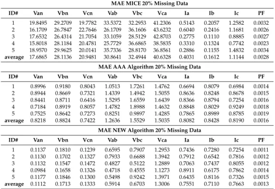
The results obtained when the MAE metric is applied to the three algorithms are equivalent. Table5shows the results obtained using the MAE metric for 10% missing data, while Table6does the same for 15% and Table7for 20%. When the algorithm proposed is compared with AAA in the case of 10% missing data, the average of improvement regarding the MAE metric is 35%, with a minimum value of 10%. For the case of 15% missing data, the average improvement of the MAE is 29%, with a minimum of an 8% improvement in one of the variables. When the amount of missing data is 20%, the average improvement of the referenced metric is 42%, with a minimum amount of 13%.

Table 5.MAE (mean absolute error) obtained with 10% missing data using MICE, AAA and the newly proposed algorithm, HAAA.

MAE MICE 10% Missing Data

1 16.5255 27.4609 17.6382 31.0773 31.8032 39.9026 0.1725 0.2588 1.3358 0.0024 2 14.6229 24.1967 20.2526 33.6486 24.1749 40.8152 0.1744 0.2355 1.3055 0.0025 3 15.1412 23.9954 19.4134 26.2969 30.7039 41.4323 0.2113 0.2623 1.3377 0.0024 4 14.0678 25.6064 17.3741 34.8765 23.4809 37.3655 0.2512 0.2306 1.3785 0.0026 5 16.0730 27.5605 17.8741 27.4130 33.2976 35.7481 0.2334 0.1752 1.4786 0.0060 average 15.2861 25.7640 18.5105 30.6624 28.6921 39.0528 0.2086 0.2325 1.3672 0.0032

MAE AAA Algorithm 10% Missing Data

1 0.8120 0.8681 0.7423 0.4379 1.3656 2.5745 0.1117 0.1210 0.9243 0.0059 2 0.8358 0.8545 0.7946 1.5311 1.2375 0.8110 0.1210 0.1228 1.0954 0.0062 3 0.8274 0.8546 0.7923 1.1356 1.4964 1.3782 0.1215 0.1272 0.9566 0.0095 4 0.8653 0.8651 0.7562 1.3314 1.4677 1.3657 0.1186 0.1222 1.0425 0.0085 5 0.9052 0.8561 0.7563 1.2364 1.2115 0.8277 0.1145 0.1177 0.9595 0.0120 average 0.8491 0.8597 0.7684 1.1345 1.3557 1.3914 0.1175 0.1222 0.9957 0.0084

MAE New Algorithm 10% Missing Data

1 0.8192 0.7406 0.6883 0.3447 0.5175 1.0331 0.1047 0.1091 0.1338 0.0042 2 0.6789 0.6371 0.7580 0.5359 0.5140 1.0838 0.1163 0.0872 0.1410 0.0033 3 0.7080 0.6473 0.7381 0.4839 0.3278 1.0783 0.0923 0.1055 0.1387 0.0054 4 0.6946 0.7001 0.6387 0.5285 0.2821 0.8947 0.1224 0.0845 0.1253 0.0049 5 0.7616 0.7693 0.6695 0.1723 0.6028 1.0647 0.0926 0.1158 0.1217 0.0069 average 0.7325 0.6989 0.6985 0.4131 0.4488 1.0309 0.1057 0.1004 0.1321 0.0049

(9)

Table 6. MAE obtained with 15% missing data using MICE, AAA and the newly proposed algorithm, HAAA.

1 17.1855 27.7909 18.2982 32.3532 40.3426 31.4073 0.7919 0.9918 2.0018 0.0149 2 15.2829 24.4167 20.6926 24.3949 41.2552 34.0886 1.0895 0.9905 2.0695 0.0141 3 15.5812 24.6554 19.6334 31.0339 41.9823 26.7369 0.3773 0.6813 2.0927 0.0171 4 14.6178 26.0464 17.8141 23.7009 37.6955 35.2065 0.5732 0.5966 1.8180 0.0189 5 16.2930 27.8905 18.5341 33.9576 35.9681 27.6330 0.4885 1.2168 2.1226 0.0205 average 15.7921 26.1600 18.9945 29.0881 39.4488 31.0144 0.6641 0.8954 2.0209 0.0171

1 0.9321 0.9516 0.8651 1.3788 1.4240 1.3866 0.0932 0.0952 0.0865 0.0063 2 0.9576 0.8613 0.9000 1.3569 1.3313 1.3687 0.0958 0.0861 0.09 0.0075 3 0.5774 0.8965 0.8652 1.3458 1.5144 1.3788 0.0577 0.0896 0.0865 0.0101 4 0.9626 0.8945 0.9513 1.3565 1.5227 1.3744 0.0963 0.0895 0.0951 0.0096 5 0.9342 0.9852 0.9806 1.3026 1.5278 1.3506 0.0934 0.0985 0.0981 0.0124 average 0.8728 0.9178 0.9125 1.3481 1.4640 1.3718 0.0873 0.0918 0.0912 0.0092

1 0.7185 0.5040 0.6644 0.4819 0.5835 1.0881 0.0797 0.0851 0.0842 0.0072 2 0.5999 0.4390 0.7368 0.5861 0.5800 1.1278 0.0882 0.0699 0.0881 0.0056 3 0.6245 0.4420 0.7256 0.2459 0.3938 1.1113 0.0696 0.0839 0.0881 0.0093 4 0.6131 0.4770 0.6181 0.3534 0.3371 0.9497 0.0927 0.0684 0.0789 0.0086 5 0.6783 0.5150 0.6615 0.2834 0.6578 1.1307 0.0709 0.0908 0.0771 0.0114 average 0.6469 0.4754 0.6813 0.3902 0.5104 1.0815 0.0802 0.0796 0.0833 0.0084

Table 7. MAE obtained with 20% missing data using MICE, AAA and the newly proposed algorithm HAAA.

1 19.8495 29.2709 19.7782 33.5372 32.2953 41.2306 0.5143 0.2057 1.2582 0.0032 2 16.1709 26.7847 22.7646 26.1709 36.1606 43.6232 0.6040 0.2416 1.1681 0.0026 3 17.6532 26.4314 21.7054 33.1059 28.5129 42.8703 0.2775 0.1110 0.8885 0.0027 4 15.8018 28.1184 20.4781 25.7729 36.6865 38.5835 0.3310 0.1324 0.7742 0.0023 5 18.9570 29.9625 20.0141 35.7336 28.8170 36.8561 0.2886 0.1155 1.4832 0.0034 average 17.6865 28.1136 20.9481 30.8641 32.4944 40.6328 0.4031 0.1612 1.1144 0.0028

1 0.8996 0.9180 0.8043 1.0513 1.7261 1.4762 0.6694 0.8079 0.6984 0.0014 2 0.8944 0.8669 0.7321 1.4339 1.4942 1.5055 0.8636 0.8248 0.8678 0.0015 3 0.8441 0.8711 0.6416 1.5295 1.6559 1.6439 0.8366 0.8794 0.7254 0.0016 4 0.7184 0.8919 0.8057 1.4782 1.8988 1.4632 0.8848 0.8029 0.9249 0.0018 5 0.7525 0.8642 0.7273 0.8251 0.9897 1.4285 0.7865 0.8989 0.8785 0.0019 average 0.8218 0.8824 0.7422 1.2636 1.5529 1.5035 0.8082 0.8428 0.8190 0.0016

MAE NEW Algorithm 20% Missing Data

1 0.1137 0.1810 0.1239 0.6595 0.7907 1.2953 0.7436 0.7280 0.7254 0.0011 2 0.1130 0.1702 0.1327 0.7933 0.6688 1.3942 0.7912 0.6542 0.7816 0.0012 3 0.1132 0.1547 0.1472 0.4827 0.5122 1.2889 0.7063 0.7437 0.8055 0.0012 4 0.0984 0.1658 0.1326 0.4718 0.4555 1.1273 0.8911 0.6175 0.7862 0.0014 5 0.1177 0.1846 0.1300 0.5498 0.9242 1.3971 0.6435 0.8116 0.7326 0.0015 average 0.1112 0.1713 0.1333 0.5914 0.6703 1.3006 0.7551 0.7110 0.7663 0.0013

Although the overall performance of the new algorithm has already been evaluated using MCAR data, from the point of view of the authors, there are a couple of situations in which the information is not missing completely at random and are of great interest for electrical measurements. These are as follows:

(10)

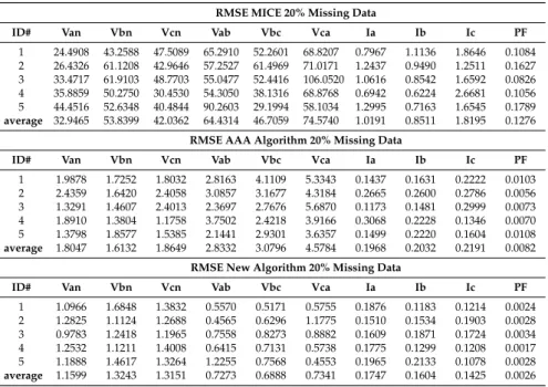
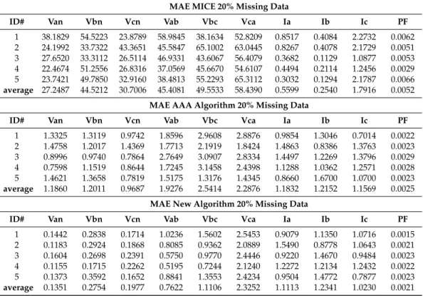
• The case in which there is correlation in the missingness of data: one possible situation when working with electrical data would be when all the missing information corresponds to the same phase. In order to simulate this kind of failure, five new data sets with a 20% of missing data were created. Each phase is represented by means of four different variables: one variable of phase current, two variables of voltage from phase to phase and one variable of voltage from phase to neutral. It means that each row with missing incomplete information has four missing variables or, in other words, that only 5% of the total of rows will have missing data. In the referred rows, randomly selected, the information of the variables of one of the phases was removed. It means that, for example, when information for variableVanis missing, it is also missing the information of variables,Vab,Vca and Ia. The results obtained are presented in Tables9and10. As it can be observed, the performance of the HAAA algorithm is worse than in the MCAR case, but it outperforms both MICE and AAA.

• The case in which most of the missing data correspond to a certain subset of variables. In order to simulate this kind of failure, five new datasets with a 90% of missing data in a single variable were created. In each dataset, a proportion of 90% elements in one single column were removed, leaving the rest of the variables with their original values. As it can be seen in Table 8, the imputation accuracy for all the algorithms decreased significantly. This was expected in such an unfavourable situation; however, it is possible to ascertain, as both algorithms HAAA and AAA considerably outperform the algorithm of reference MICE, HAAA being the one with the best results.

Table 8. MAE and RMSE obtained with 90% missing data in a single column (case of missing information in Van) using MICE, AAA and the newly proposed algorithm HAAA.

ID#

90% Missing Data in One Single Columm MAE RMSE

MICE AAA HAAA MICE AAA HAAA

1 87.1375 10.2289 8.9960 103.8879 12.3165 8.7614 2 68.0226 10.1661 8.9438 99.2328 12.8503 8.6589 3 76.3340 10.1900 8.4414 86.4040 11.8568 9.1133 4 67.0027 8.8589 7.1839 90.5413 10.5458 7.9936 5 82.5461 10.5940 7.5248 102.5351 13.6865 9.5870 average 76.2086 10.0076 8.2180 96.5202 12.2512 8.8228

Table 9.RMSE obtained with 20% missing data using MICE, AAA and the newly proposed algorithm, HAAA for the case in which there is correlation in the missingness of data.

1 24.4908 43.2588 47.5089 65.2910 52.2601 68.8207 0.7967 1.1136 1.8646 0.1084 2 26.4326 61.1208 42.9646 57.2527 61.4969 71.0171 1.2437 0.9490 1.2511 0.1627 3 33.4717 61.9103 48.7703 55.0477 52.4416 106.0520 1.0616 0.8542 1.6592 0.0826 4 35.8859 50.2750 30.4530 54.3050 38.1316 68.8768 0.6942 0.6224 2.6681 0.1056 5 44.4516 52.6348 40.4844 90.2603 29.1994 58.1034 1.2995 0.7163 1.6545 0.1789 average 32.9465 53.8399 42.0362 64.4314 46.7059 74.5740 1.0191 0.8511 1.8195 0.1276

1 1.9878 1.7252 1.8032 2.8163 4.1109 5.3343 0.1437 0.1631 0.2222 0.0103 2 2.4359 1.6420 2.4058 3.0857 3.1677 4.3184 0.2665 0.2600 0.2786 0.0056 3 1.3291 1.4607 2.4013 2.3697 2.7676 5.6870 0.1173 0.1481 0.2999 0.0073 4 1.8910 1.3804 1.1758 3.7502 2.4218 3.9166 0.3068 0.2228 0.1346 0.0070 5 1.3798 1.8577 1.5385 2.1441 2.9301 3.6357 0.1499 0.2220 0.1604 0.0108 average 1.8047 1.6132 1.8649 2.8332 3.0796 4.5784 0.1968 0.2032 0.2191 0.0082

1 1.0966 1.6848 1.3832 0.5570 0.5171 0.5755 0.1876 0.1183 0.1214 0.0024 2 1.2825 1.1124 1.2688 0.4565 0.6296 1.1775 0.1510 0.1534 0.1903 0.0028 3 0.9783 1.2418 1.1965 0.7558 0.8273 0.8882 0.1609 0.1871 0.1724 0.0034 4 1.2532 1.1211 1.4008 0.6415 0.7131 0.5738 0.1775 0.1299 0.1208 0.0017 5 1.1888 1.4617 1.3264 1.2255 0.7568 0.4553 0.1965 0.2133 0.1078 0.0028 average 1.1599 1.3243 1.3151 0.7273 0.6888 0.7341 0.1747 0.1604 0.1425 0.0026

(11)

Table 10.MAE obtained with 20% missing data using MICE, AAA and the newly proposed algorithm HAAA for the case in which there is correlation in the missingness of data.

1 38.1829 54.5223 23.8789 58.9845 38.1634 52.8209 0.8517 0.4084 2.2732 0.0062 2 24.1992 33.7322 43.3651 45.5847 65.1002 63.0445 0.8267 0.4078 2.1729 0.0051 3 27.6520 33.3112 26.5114 46.9331 43.6067 56.4079 0.3682 0.1129 1.0877 0.0053 4 22.4674 51.2556 26.8316 37.0569 45.6670 54.6107 0.4494 0.2114 1.2456 0.0029 5 23.7421 49.7850 32.9160 38.4813 55.2293 65.3112 0.3032 0.1294 2.1787 0.0066 average 27.2487 44.5212 30.7006 45.4081 49.5533 58.4390 0.5599 0.2540 1.7916 0.0052

1 1.3325 1.3119 0.9742 1.8596 2.9608 2.8876 0.9854 1.3046 0.7014 0.0022 2 1.4758 1.2017 1.4369 1.7713 2.1919 1.8424 1.4863 0.8386 1.3763 0.0023 3 0.8996 0.9740 0.7864 2.7649 3.0907 2.8334 1.4497 1.2269 1.3796 0.0029 4 0.7598 1.1519 0.8644 1.7245 3.1458 2.4398 1.1288 1.0362 1.2571 0.0028 5 1.4621 1.3658 0.7819 1.5175 1.3176 1.4345 0.8660 1.6700 1.0700 0.0023 average 1.1860 1.2011 0.9687 1.9276 2.5414 2.2876 1.1832 1.2152 1.1569 0.0025

1 0.1442 0.2838 0.1714 1.0236 1.5602 2.5453 0.9079 1.1350 1.0716 0.0015 2 0.1183 0.2924 0.1868 0.8085 0.9362 2.0889 1.5490 0.8778 1.0643 0.0021 3 0.1604 0.2698 0.2391 0.5750 0.9770 2.4446 0.9220 1.4670 0.9484 0.0023 4 0.1155 0.1715 0.2262 0.5195 0.7244 2.1240 1.2272 1.2134 1.2432 0.0022 5 0.1373 0.3592 0.1652 0.8841 1.3553 2.4234 0.9504 1.4772 0.7877 0.0023 average 0.1351 0.2754 0.1977 0.7622 1.1106 2.3252 1.1113 1.2341 1.0230 0.0021 5. Conclusions

The improvement of power quality has become a necessity as the presence of power electronics in today’s grids has been increasing in the last decades. Due to this problem, network monitoring with the help of real-time data collection devices is helpful. In this context, the availability of missing data imputation techniques is required.

This research presents a new algorithm and compares it with another algorithm proposed in a previous paper by the authors and also with a well-known missing data imputation algorithm. Although the algorithm presented in this paper outperforms the others, as the previous methods to which it is compared, it also has some limitations that must be taken into account. As those proposed before, our algorithm would have imputation problems in those cases in which most of the missing data belonged to the same variable or were concentrated in a certain subset of variables instead of distributed among all the variables of the data set. Currently, the authors continue to develop hybrid algorithms that would improve the results of existing algorithms when they have to address this type of issue. Finally, the missing data imputation in the time-frequency domain will also be explored in future works.

Acknowledgments:Francisco Javier de Cos Juez and Fernando Sánchez Lasheras appreciate support from the Spanish Economics and Competitiveness Ministry, through grant AYA2014-57648-P and the Government of the Principality of Asturias (Consejería de Economía y Empleo), through grant FC-15-GRUPIN14-017.

Author Contributions:Francisco Javier de Cos Juez, Concepción Crespo Turrado and Fernando Sánchez Lasheras conceived the study. Andrés José Piñón Pazos and José Luis Calvo Rollé programmed the required algorithms. Fernando Sánchez Lasheras, Manuel G. Melero and Francisco Javier de Cos Juez interpreted the results and drafted the manuscript; Concepción Crespo Turrado, Andrés José Piñón Pazos, Manuel G. Melero and José Luis Calvo Rollé supervised the experimental data analysis; and they also contributed to the critical revision and improvement of the paper. All of the authors have approved the final version of the manuscript.

(12)

References

1. Chattopadhyay, S.; Mitra, M.; Sengupta, S. Electric power quality. InElectric Power Quality; Springer: Dordrecth, The Netherlands, 2011; pp. 5–12.

2. Dixit, J.B.; Yadav, A.Electrical Power Quality; University Science Press: New Delhi, India, 2010. 3. Stones, J.; Collinson, A. Power quality.Power Eng. J.2001,15. [CrossRef]

4. Ferreira, D.D.; de Seixas, J.M.; Cerqueira, A.S.; Duque, C.A.; Bollen, M.H.J.; Ribeiro, P.F. A new power quality deviation index based on principal curves.Electr. Power Syst. Res.2015,125, 8–14. [CrossRef]

5. Mahela, O.P.; Shaik, A.G.; Gupta, N. A critical review of detection and classification of power quality events.

Renew. Sustain. Energy Rev.2015,41. [CrossRef]

6. Granados-Lieberman, D.; Valtierra-Rodriguez, M.; Morales-Hernandez, L.; Romero-Troncoso, R.; Osornio-Rios, R. A hilbert transform-based smart sensor for detection, classification, and quantification of power quality disturbances.Sensors2013,13, 5507–5527. [CrossRef] [PubMed]

7. Granados-Lieberman, D.; Romero-Troncoso, R.J.; Cabal-Yepez, E.; Osornio-Rios, R.A.; Franco-Gasca, L.A. A real-time smart sensor for high-resolution frequency estimation in power systems.Sensors2009,9, 7412–7429. [CrossRef] [PubMed]

8. Lim, Y.; Kim, H.-M.; Kang, S. A design of wireless sensor networks for a power quality monitoring system.

Sensors2010,10, 9712–9725. [CrossRef] [PubMed]

9. Crespo Turrado, C.; Sánchez Lasheras, F.; Calvo-Rolle, J.L.; Piñón-Pazos, A.J.; de Cos Juez, F.J. A new missing data imputation algorithm applied to electrical data loggers. Sensors2015,15, 31069–31082. [CrossRef]

[PubMed]

10. Electro Industries, Gauge Tech. Index of Products. Available online: http://www.electroind.com/products/ (accessed on 13 November 2015).

11. Sánchez Lasheras, F.; Nieto, P.; de Cos Juez, F.; Bayón, R.; Suárez, V. A hybrid PCA-CART-MARS-based prognostic approach of the remaining useful life for aircraft engines.Sensors2015,15, 7062–7083. [CrossRef]

[PubMed]

12. De Andres, J.; Lorca, P.; Sánchez-Lasheras, F.; de Cos Juez, F.J. Bankruptcy prediction and credit scoring: A review of recent developments based on hybrid systems and some related patents.Rec. Pat. Comp. Sci.2012, 5, 11–20. [CrossRef]

13. Chai, T.; Draxler, R.R. Root mean square error (RMSE) or mean absolute error (MAE)?—Arguments against avoiding RMSE in the literature.Geosci. Model Dev.2014,7, 1247–1250. [CrossRef]

14. Turrado, C.; López, M.; Sánchez Lasheras, F.; Gómez, B.; Rollé, J.; de Cos Juez, F.J. Missing data imputation of solar radiation data under different atmospheric conditions.Sensors2014,14, 20382–20399. [CrossRef]

[PubMed]

15. Kohonen, T.Self-Organizing Maps, 1st ed.; Springer: Berlin, Germany; Heidelberg, Germany, 1995.

16. De Andres, J.; Sánchez-Lasheras, F.; Lorca, P.; de Cos Juez, F.J. A hybrid device of self organizing maps (SOM) and multivariate adaptive regression splines (MARS) for the forecasting of firms’ bankruptcy.J. Account.

Manag. Inf. Syst.2011,10, 351–374.

17. Sánchez-Lasheras, F.; de Andrés, J.; Lorca, P.; de Cos Juez, F.J. A hybrid device for the solution of sampling bias problems in the forecasting of firms’ bankruptcy.Expert Syst. Appl.2012,39, 7512–7523. [CrossRef] 18. García Nieto, P.J.; Alonso Fernández, J.R.; Sánchez Lasheras, F.; de Cos Juez, F.J.; Díaz Muñiz, C. A new

improved study of cyanotoxins presence from experimental cyanobacteria concentrations in the Trasona reservoir (Northern Spain) using the MARS technique. Sci. Total Environ. 2012,430, 88–92. [CrossRef]

[PubMed]

19. De Cos Juez, F.J.; Sánchez Lasheras, F.; García Nieto, P.J.; Suarez, M.A.S. A new data mining methodology applied to the modelling of the influence of diet and lifestyle on the value of bone mineral density in post-menopausal women.Int. J. Comput. Math.2009,86, 1878–1887. [CrossRef]

(13)

20. Suárez Sánchez, A.; Riesgo Fernández, P.; Sánchez Lasheras, F.; de Cos Juez, F.J.; García Nieto, P.J. Prediction of work-related accidents according to working conditions using support vector machines.

Appl. Math. Comput.2011,218, 3539–3552. [CrossRef]

21. De Cos Juez, F.J.; Sánchez Lasheras, F.; Roqueñí, N.; Osborn, J. An ANN-based smart tomographic reconstructor in a dynamic environment.Sensors2012,12, 8895–8911. [CrossRef] [PubMed]

© 2016 by the authors; licensee MDPI, Basel, Switzerland. This article is an open access article distributed under the terms and conditions of the Creative Commons Attribution (CC-BY) license (http://creativecommons.org/licenses/by/4.0/).