The Canadian Journal of Statistics Vol. 33, No 3, 2005, Pages ???–??? La revue canadienne de statistique
Local dependence estimation using
semiparametric Archimedean copulas
Fran¸cois VANDENHENDE and Philippe LAMBERT
Key words and phrases: Archimedean copula; local dependence; quantile function; semiparametric smoothing.
MSC 2000: Primary 62N02, 62H12, 62G05; secondary 62H20.
Abstract: The authors define a new semiparametric Archimedean copula family having a flexible depen-dence structure. The family’s generator is a local interpolation of existing generators. It has locally-defined dependence parameters. The authors present a penalized constrained least-squares method to estimate and smooth these parameters. They illustrate the flexibility of their dependence model in a bivariate survival example.
Estimation de la d´ependance locale sur base de copules archim´ediennes semiparam´etriques
R´esum´e : Les auteurs d´efinissent une nouvelle famille de copules archim´ediennes semiparam´etriques dont la structure de d´ependance est flexible. Le g´en´erateur de la famille est une interpolation locale de g´en´era-teurs existants. Ses param`etres de d´ependance sont d´efinis localement. Les aug´en´era-teurs pr´esentent une m´ethode de moindres carr´es contraints p´enalis´es permettant l’estimation lisse de ces param`etres. Ils illustrent la flexibilit´e de leur mod`ele de d´ependance dans un exemple de survie bivari´ee.
1. INTRODUCTION
The Archimedean copula family (Genest & MacKay 1986; Nelsen 1999, Chapter 4) is an important class of dependence functions that can be used to generate joint distributions of random variablesX1 andX2
with specified marginal distributionsFX1(x1) = P(X1≤x1) andFX2(x2) = P(X2≤x2). Members of this
class are bivariate distributionsCwith uniform margins on [0,1]2 constructed from a continuous, strictly
decreasing, and convex functionφsuch that
C(u, v) =φ[−1]{φ(u) +φ(v)}, u, v∈[0,1].
The functionφis called the generator of the copula. Then,
H(x1, x2) =C{FX1(x1), FX2(x2)}
is the joint distribution of (X1, X2). The strength of dependence betweenX1 andX2 is a function of the
shape ofC.
Genest & Rivest (1993, 2001) derived the distribution function
K(p) = P{C(U, V)≤p}
of the probability integral transformationC(U, V) associated with a pair (U, V) of uniform random variables with Archimedean copulaC. For anyp∈[0,1], it is equal to
K(p) =p− φ(p)
where φ0(p+) denotes the right-derivative ofφ atp. One rank-based dependence measure, Kendall’s tau
(Kruskal 1958), is derived from that distribution. WhenX1 andX2 are absolutely continuous, Genest &
MacKay (1986) showed that
τ = 4E{C(U, V)} −1 = 1 + 4 Z 1
0
φ(p)
φ0(p+)dp. (1)
This global concordance measure has a simple interpretation. It estimates the difference between the probabilities of concordance and discordance in (X1, X2). With Archimedean copulas,τis a direct function
of the generatorφ.
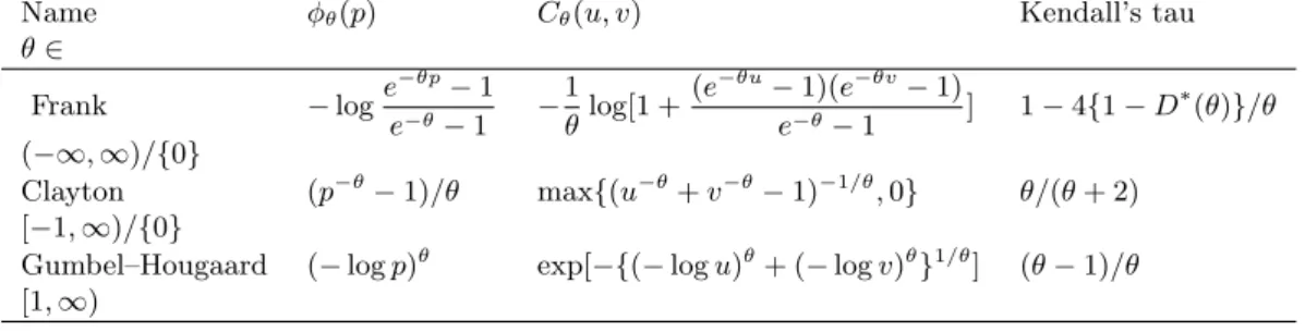
The class of Archimedean copulas encompasses many well-known bivariate parametric distributions (see, e.g., Nelsen 1999, pp. 94–97), such as the families of Frank, Clayton or Gumbel–Hougaard given in Table 1. For these families, the generator φ has a single parameter θ that measures the sign and the strength of the dependence. In every case, one specific (possibly limiting) value forθleads to the generator
φ(p) =−log(p) that creates independence, as then,C= exp{log(U) + log(V)}=U V is the product of the marginsU andV. For each of these families, there is a one-to-one mapping betweenθ andτ, as given in Table 1. A three-parameter family including as special cases the various copulas from this table was given by Genest, Ghoudi & Rivest (1998).
Table 1. Selected bivariate Archimedean copulas having a single dependence parameterθ. Name φθ(p) Cθ(u, v) Kendall’s tau
θ∈ Frank −loge −θp−1 e−θ−1 − 1 θlog[1 + (e−θu−1)(e−θv−1) e−θ−1 ] 1−4{1−D ∗ (θ)}/θ (−∞,∞)/{0} Clayton (p−θ−1)/θ max{(u−θ+v−θ−1)−1/θ,0} θ/(θ+ 2) [−1,∞)/{0}
Gumbel–Hougaard (−logp)θ exp[−{(−logu)θ+ (−logv)θ}1/θ] (θ−1)/θ [1,∞)
*: D(x) =x−1 Rx 0
t
et−1dtis the Debye function.
In practical problems, one can estimate easily the dependence parameter by equating the sample-based estimate of Kendall’s tau to its population version from Table 1. Asτ is a function of the first moment ofK
(see Equation 1), the estimation can be seen as a moment-based method. Other methods such as inversion of Spearman’s rho or pseudo-maximum likelihood (ML) are also possible; the latter was studied by Genest, Ghoudi & Rivest (1995) and by Shih & Louis (1995). See, for instance, Vandenhende & Lambert (2000) for an application.
The selection of an Archimedean family is often arbitrary and rarely automated. Genest & Rivest (1993) provided a graphical method allowing the comparison of different parametric distributionsKwith the empirical counterpart. In Vandenhende & Lambert (2000), copula selection was done using Akaike’s information criteria from the ML fit of several copula models having the same marginal components. In the two cases, only a limited set of families are investigated.
In this paper, we overcome this selection problem by defining flexible semiparametric Archimedean cop-ulas. The distributionK is estimated using local polynomials whose coefficients quantify the dependence locally. The layout is as follows. As a preamble, in Section 2, we relate Archimedean copulas to univariate quantile functions. In Section 3, we define the semiparametric Archimedean copula family. Dependence properties of parameters are discussed in Section 4. The estimation and smoothing of parameters are presented in Section 5. The practical usefulness of the semiparametric copula is illustrated in Section 6. Section 7 contains a discussion of key results.
2. ARCHIMEDEAN COPULAS AND QUANTILE FUNCTIONS
Theorem 1 shows a simple way to create univariate continuous distributions from any copula in the Archimedean family. It also summarizes a list of log-linear composition rules of Archimedean genera-tors to enrich the bivariate Archimedean family (Genest, Ghoudi & Rivest, 1998).
Theorem 1. Letφ(p) be the generator of an Archimedean copula. Forp∈[0,1], let
S(p) =−log{φ(p)} and Q(p) =c+θS(p), (2)
for anyc∈Randθ >0. Then,
a) S andQare valid univariate quantile functions for a continuous random variableZ inR.
b) Ifφ is strict, i.e., ifφ(0) = +∞, then the domain ofZ is unbounded inR; otherwise it is bounded to the left.
c) If the mean µS and variance vS of S exist, the mean and variance derived from Q are equal to
µQ=c+θµS andvQ=θ2vS, respectively.
d) exp(−Q)is an Archimedean generator when θ≥1. It generates the same copula asexp(−S)when
θ= 1 (whateverc∈R).
The construction in (2) can be applied recursively to create new quantile functions Qfrom a seriesS1, . . . , Sn of log-generators. Then, exp(−Q) is an Archimedean generator when allθi ≥1.
3. SEMIPARAMETRIC ARCHIMEDEAN COPULAS
Instead of combining multiple log-generatorsSi on the whole [0,1] range, one can assemble several functions Si, each being defined locally on a sub-interval [ti, ti+1) from a partition of [0,1]. The
resultQis a local linear combination of the Si. Under some conditions, it is such that exp(−Q) generates an Archimedean copula. That copula is indeed a semiparametric (or highly parameter-ized) Archimedean copula, having parameters that quantify the dependence locally. In this section, we detail how to accomplish this.
Theorem 2. Let t1, . . . , tn be nknots such that 0< t1<· · ·< tn<1. Two additional knots are
defined at t0 = 0 and tn+1 >1. LetS =−log(φ)with φ being any Archimedean generator. We define the local polynomialQas
Q(p) = n X
i=0
{θ0,i+θiS(p)}I(ti≤p < ti+1). (3)
Thenexp(−Q)is an Archimedean generator whenever
(i) fori= 1, . . . , n,θ0,i= Pi
k=1S(tk)(θk−1−θk), and (ii) 1≤θn≤ · · · ≤θ0.
The resulting copula has the following properties:
a) The same copula is generated whatever θ0,0. One can thus set θ0,0= 0, arbitrarily.
b) exp(−Q) is a strict generator if and only ifexp(−S)is strict.
c) The semiparametric copula hasn+ 1dependence parametersθ0, . . . , θn, supplementing those
from S. Each parameterθi quantifies locally the dependence in [ti, ti+1).
d) Q is almost surely twice differentiable, except at the knotst1, . . . , tn, where it is continuous. e) Q is differentiable at the knotti when θi−1=θi.
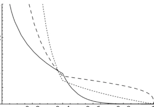
0.2 0.4 0.6 0.8 1 p 0.5 1 1.5 2 2.5 3 phi
Figure 1. The generator φ= exp(−Q) with Q defined in (3) based onS(p) =−log{−log(p)},
n= 1, andt1= 0.4 is convex whenθ0= 4 andθ1= 1 (dotted line). It is not convex when (θ0, θ1)
equals (1,4) (solid line) or (2,0.3) (dashed line).
The condition on the intercepts ensures the continuity of Q at the knots. As illustrated in Figure 1, the decreasing ordering condition 1≤θn≤ · · · ≤θ0 is necessary to ensure the convexity
of the resulting generator.
The function Qdefined in (3) uses a single function S across all intervals. Thus, its inverse
Q−1(x) = n X i=0 S−1 µ x−θ0,i θi ¶ I{Q(ti)≤x < Q(ti+1)}
has an explicit form whenS−1 is itself explicit.
Then, the bivariate copula having exp(−Q) as generator is
C(u, v) = n X i=0 S−1 µ x−θ0,i θi ¶ I{Q(ti)≤x < Q(ti+1)}, (4) where x = −log " exp " − n X i=0 {θ0,i+θiS(u)}I(ti≤u < ti+1) # + exp " − n X i=0 {θ0,i+θiS(v)}I(ti≤v < ti+1) ## .
It has a closed-form expression when the copula generated by exp(−S) has an analytical form. One particular but important choice is when exp(−S) generates independence, namelyS(p) =
−log{−log(p)}. Then,
exp{−Q(p)}= n Y
i=0
£
e−θ0,i{−log(p)}θi¤I(ti≤p<ti+1) (5)
is locally, on [ti, ti+1), a Gumbel–Hougaard (θi) generator (see Table 1). The resulting bivariate copula has a simple closed-form expression. It generates independence when allθi= 1.
4. DEPENDENCE PROPERTIES
We now study dependence properties of the semiparametric Archimedean copula defined in Section 3. With the copula defined in (4), Kendall’s tau from (1) becomes
τ = 1−4 n X i=0 1 θi Z ti+1 ti 1 S0(p+)dp.
Since it must be thatθi ≥1 for all 0≤i≤n, the larger any local parameterθi, the larger τ will be. WhenS does not contain any dependence parameter, the integral part can be seen as a weight factor associated to eachθi in the sum.
With the locally Gumbel–Hougaard copula discussed previously, i.e., when S =−log(−log), Kendall’s tau becomes
τ = n X i=0 wiθi−1 θi , with wi={t2i+1(1−2 logti+1)−t2i(1−2 logti)} withw0+· · ·+wn= 1. It is a weighted sum of locally-defined parameters
τi=θi−1
θi . (6)
Eachτi is indeed equal to Kendall’s tau for the Gumbel–Hougaard (θi) copula defined on [ti, ti+1)
(See Table 1). A local dependence interpretation of parameters is thus possible in this particular case.
The weights wi depend on the location of the knots. The larger the size of an interval, the larger the corresponding weight. With equidistant knots, the wi have a bell-shaped curve having a maximum in the unit interval. The location of this maximum depends on the distance between knots in a non-algebraic way. Numerical procedures can also help to determine the series ofn+ 1 knots that produces equal weights wi = 1/n. For instance, with n= 10, weights are equal with interior knots at{0.14, 0.22, 0.30, 0.36, 0.43, 0.50, 0.58, 0.66, 0.77}.
5. ESTIMATION PROCEDURE
In this section, we first observe that the distributionKof our new copula is linear in the (inverse) dependence parameters. This enables the estimation of parameters using a fast (constrained) least-squares procedure. We also show how to reduce, and even optimize the effective number of parameters, by smoothing the dependence over successive sub-intervals. Finally, we approximate the distribution of parameters using a bootstrap method.
5.1. Least-squares estimation.
Let (X1, X2) be a bivariate random vector for whichmobservations are available. Genest & Rivest
(1993) showed that their joint empirical distribution at (X1,k, X2,k) isVk (k= 1, . . . , m), where
Vk= #{(X1,j, X2,j)≤(X1,k, X2,k)}/m. (7) Therefore, the empirical counterpart ofKis the step functionKm(V), such that for allV ∈R,
Km(V) = #(Vj≤V)/m.
With the semiparametric bivariate copula (4),K becomes K(p) =p+ 1 S0(p+) n X i=0 1 θi I(ti≤p < ti+1).
It is linear in the inverse dependence parameters 1/θi, whatever the choice ofS. For instance, with the locally Gumbel–Hougaard generator (5),
K(p) =p−plog(p) n X i=0 1 θi I(ti≤p < ti+1).
As discussed by Genest & Rivest (1993), a graphical comparison of the plot ofK(p)−pversus
pto its empirical counterpart is informative to assess whether the dependence has an Archimedean structure. In the Archimedean class,K(p)−pis always positive and has a first order derivative greater than or equal to−1 on all [0,1]. That plot can also assess if a particular model fits well to the data. See Figure 3(a) for an example of good Archimedean fit.
Using a simple reparameterisation βi = 1/θi, parameters can then be estimated based on the comparison ofKmtoKacross all observed joint proportionsV1, . . . , Vm. AnL2–norm comparison
yields estimates b βi= arg min m X k=1 ( Km(Vk)−Vk− 1 S0(V+ k ) n X i=0 βiI(ti≤Vk< ti+1) )2 withβ0≤ · · · ≤βn≤1.
In matrix notations, we define the pseudo-observation m-vector
Y ={Km(Vk)−Vk, j= 1, . . . , m} and them×(n+ 1) design matrix
X ={1/S0(Vk+)I(ti≤Vk< ti+1), i= 0, . . . , n, k= 1, . . . , m}.
Then+ 1 inequality constraints β0 ≤ · · · ≤ βn ≤1 can be expressed as A>β ≥0 for an appro-priate choice ofA. The estimation problem becomes a simple constrained least-squares estimation procedure
argβmin(Y −Xβ)>(Y −Xβ), withA>β ≥0.
5.2. Smoothing and optimizing the dependence.
Our copula model has as many parameters as there are knots. Furthermore, the location of the knots has an influence on the parameter estimates. With no interior knot (n = 0), a single and constant dependence parameter is estimated, and the least-squares method becomes an alternative to the moment-based estimator presented in Section 1. When knots are placed at all distinct
V1, . . . , Vm, this becomes a (constrained) interpolation problem. The level of smoothing of the fit increases as the number of knots decreases. It also increases when the estimates of parameters corresponding to successive knots are constrained to be similar.
Here, we propose to consider many equidistant knots and to control the smoothness of the fit by adding a penalty term to the least-squares problem. We follow Eilers & Marx (1996) and minimize the constrained penalized least squares
with ∆rβ that contains the rth order finite differences between successive parameters. It builds up recursively from ∆1β = (β1−β0, . . . , βn−βn−1)> to create ∆rβ = ∆(∆r−1β). The penalty λdetermines the level of smoothing that is desired in the fit. A value λ= 0 corresponds to the constrained interpolation case with no smoothing. The correctionr= 1 is a first-order correction as it tends to penalize any linear change in successive dependence parameters. Whenλ→+∞, a constant dependence parameter is estimated (one degree of freedom is left). Withr= 2, quadratic changes are penalized, so that whenλ→+∞, only a linear change of dependence is possible over the sub-intervals. The effective number of parameters is at most 2 in that case. It can actually be lower than 2, when constraints are activated. Although higher-order penalties are possible, taking
r= 2 seems in general appropriate for most practical problems.
The optimization problem (8) can be solved using a quadratic programming algorithm with lin-ear inequality constraints (Gill, Murray & Wright, 1981). We used the dual method of Goldfarb & Idnani (1983), implemented by Andreas Weingessel in theR language (Ihaka & Gentleman, 1996) to estimate the β parameters for several values of λ. We also calculated the effective number of parameters for each fit, as in Wood (2000), and the generalized cross-validation (GCV) measure (Wahba, 1990) in the usual way. The best λvalue and the corresponding βbestimates were then selected to minimize theGCV(λ) criterion.
5.3. Variability estimation.
The constrained penalized least squares (PCLS) estimation algorithm does not tell us anything about the distributional properties of the parameter estimates. The availability of variance esti-mates for the parameter estimators and for the predictions enables to assess the quality of the fit, and to evaluate the adequacy of any parametric proposal for the Archimedean copula. We esti-mate the distribution ofβbusing the resampling-cases algorithm (Davison & Hinkley 1999, p. 264). Given the speed of the PCLS estimation algorithm, it is not too hard to use bootstrap methods to estimate variability of the parameter estimators. The procedure is as follows.
For a large number Rof replicates, 1. Sample (X∗
1,1, X2∗,1), . . . ,(X1∗,m, X2∗,m) randomly with replacement from {(X1,k, X2,k), k = 1, . . . , m}.
2. Compute the empirical joint distribution of that sampleV∗
1, . . . , Vm∗ using (7). 3. Apply the PCLS to V∗
1, . . . , Vm∗ using the original knots andλvalue, giving parameter esti-mates βb∗
r.
When R is large, the covariance matrix and standard error ofβb can be estimated using the corresponding estimates from the series ofβb∗
r, r= 1, . . . , R. Non-parametric confidence limits for the predicted valuesYb are also available using selected quantiles (2.5% and 97.5%, usually to get 95% confidence bands) in the seriesYb∗
1, . . . ,YbR∗.
An alternative and possibly more efficient bootstrap method is possible. It consists of sampling in Step 1 directly from the predicted bivariate copula, whereas the empirical joint distribution was used in the initial proposal. Steps 2 and 3 are then unchanged.
6. ILLUSTRATION IN A LIFETIME STUDY OF DANISH TWINS
The illustration is a large and non-censored cohort of 2872 pairs of Danish twins born 1870-1900. See Herskind, McGue, Holm, Sorensen, Harvald & Vaupel (1996) for more details on the data. Our interest is in the analysis of the dependence between the lifetimes of twins. A few subjects died prior to 60 years of age. The death rate of individuals is rather low and uniform in the 20
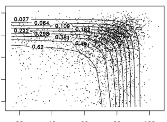
20 40 60 80 100 20 40 60 80 100 time (years) time (years)
Figure 2. Joint survival time of pairs of Danish twins. Predicted contour of the joint survival distribution using a semiparametric Archimedean copula with log-log quantile basis (λ= 10).
to 60 years interval with most deaths occurring between 60 and 90 years old. Kendall’s tau (0.11) suggests an overall moderate positive dependence between the paired survival times.
Hougaard, Harvald & Holm (1992) have applied bivariate parametric survival models to these data. Their models showed some disagreement on the way the dependence was changing with age. A scatterplot of survival times is displayed in Figure 2. That display also presents the predicted joint distribution based on our semiparametric copula model and the empirical margins. A visual inspection of Figure 2 reveals a denser cloud of points on the main diagonal from 70-years old, onwards. This might indicate that the dependence increases with joint survival times. Our formal semiparametric analysis of the dependence will confirm that observation.
Since our main interest is in the joint survival analysis of the twins, we fit the Archimedean copula models to the survival functions, instead of the distributions. To that end, we replace (7) with the joint empirical survival function
Vk= #{(X1,j, X2,j)≥(X1,k, X2,k)}/m
and follow the same estimation procedure as proposed above with that function. We setn= 100 equidistant knots and use the quantile functionS(p) =−log{−log(p)}of independence. A second-order (r= 2) penalty is chosen.
Figure 3(a) presents a PCLS fit of the semiparametric copula to Km(Vj)−Vj. The penalty in that fit (λ= 10) was chosen arbitrarily. It gives an effective number of dependence parameters of 10.3. Indeed, the GCV estimate for that model (2.7e−6) was not much larger than the optimal model (GCV = 1.6e−6;λ = 2e−4; 47.2 parms). But the drop in number of parameters was big enough to be considered. The model predictions completely overlap the empirical estimates in the plot and the confidence bands (95%) for our model cover the data everywhere. Bands were computed using the resampling-cases bootstrap method withR= 500. As expected, computation was very fast. Given the very large sample size (N = 2872), the standard error of all parameters was less that 5.8% of their mean and confidence bands were rather narrow. Despite this, the fit of the semiparametric Archimedean copula was good. With this bootstrap method, we make no assumption about variance homogeneity and dependence structure of parameters. This proves useful to put the lights on the increasing variability of model predictions with increasing probability.
0.0 0.2 0.4 0.6 0.8 1.0 0.00 0.10 0.20 0.30 p K(p)−p (a)
Semi−parametric copula with log−log basis (lambda=10) 95% confidence bands 0.0 0.2 0.4 0.6 0.8 1.0 0.00 0.10 0.20 0.30 p K(p)−p (b) Clayton Frank Gumbel
Figure 3. Empirical function Km(Vj)−Vj for the Danish twins data, superimposed with a) constrained penalized (λ= 10) least-squares fit of the semiparametric Archimedean copula with log-log quantile basis. b) fit of selected 1-parameter Archimedean copulas with dependence pa-rameter estimated from Kendall’s tau.
In Figure 3(b), the dependence parameter is estimated by equating the population version of Kendall’s tau to its sample-based estimate. The three models fit differently to the data. The larger deviation is seen in the middle of the plot (from 0.2 to 0.4). The fit of Clayton’s family is better in the other parts of the plot, although it slightly underestimates the curve at low survival probabilities.
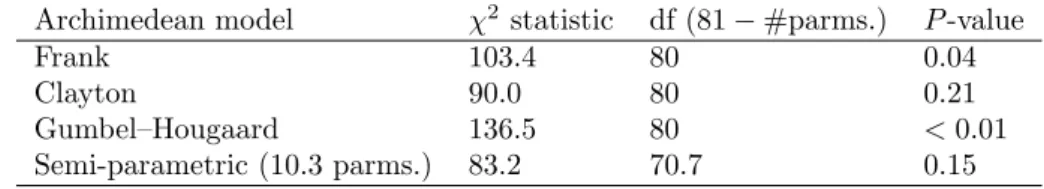
The goodness of fit of the Archimedean models was assessed using the Pearson chi-square test as implemented by Genest & Rivest (1993). The 2872 bivariate survival times were first pre-grouped into a (10x10) categorical table having interior limits at 44, 59, 67, 72, 75, 79, 82, 85, 89 years of age in each dimension. These thresholds were selected to balance frequencies among cells (mean count=28.7, range=[11,56]). The test statistics are reported in Table 2. Our flexible semiparametric Archimedean construction fits very well the data. Among the families of Table 1, Clayton’s copula provides the best one-parameter description of the bivariate dependence.
Table 2: Goodness of fit of the Archimedean models to the Danish twins survival times.
Archimedean model χ2 statistic df (81−#parms.) P-value
Frank 103.4 80 0.04
Clayton 90.0 80 0.21
Gumbel–Hougaard 136.5 80 <0.01
Semi-parametric (10.3 parms.) 83.2 70.7 0.15
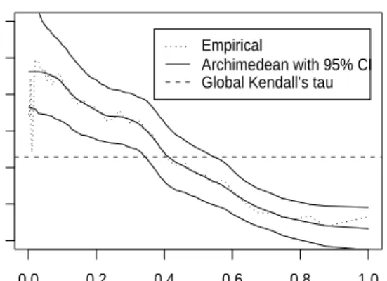
The local value of Kendall’s tau predicted from the PCLS fit of the semiparametric locally Gumbel–Hougaard Archimedean copula are in Figure 4. That model was also estimated without penalty (by setting λ = 0 instead of λ = 10) and without any monotonicity constraint on the
θi. The unconstrained fit does not necessarily produce an Archimedean copula anymore. Instead, every parameter θi is “freely” adjusted on [ti, ti+1), giving rise to the “empirical” τi estimates shown in Figure 4 (dotted line). The adequacy of the smoothed semiparametric Archimedean fit was then assessed in comparison to the empirical plot. In the illustrated example, the fit of the Archimedean model was very good. Indeed, despite its instability at lowp (i.e., when relatively few pairs are still alive), the dependence decreases with increasing survival probability. The impact of smoothing and constraining the dependence parameters was thus minimal. The global Kendall
0.0 0.2 0.4 0.6 0.8 1.0 0.00 0.10 0.20 0.30 p tau Local dependence Empirical Archimedean with 95% CI Global Kendall’s tau
Figure 4. Local dependenceτ(p) =Pi θi−1
θi I(ti≤p < ti+1) for the semiparametric Archimedean model (λ= 10) having log-log quantile basis.
tau estimate (dashed line) is close to the mean of the local dependencies, indicating that knots were well chosen to balance weightswi.
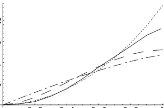
Another graphical method can be used to study the local dependence properties of our estimated copula model. Following Shih & Louis (1995), we have plotted the local correlation coefficients
r(t, t) of Prentice & Cai (1992) when the two survival times t1 =t2=tare uniform on [0,1] (see
Figure 5). All curves confirm what our local dependence measure had detected: the dependence increases with survival time, or, equivalently, it decreases with survival probability. Furthermore, the dependence curve from Figure 4 has a similar shape as the correlation curve for our semi-parametric model, when plotted versus timet= 1−p, instead of probability. The comparison of correlation curvesr(t, t) between the parametric and semiparametric models confirms the superior fit of Clayton’s copula among the one-parameter families. Our semiparametric model estimates a lower dependence than Clayton’s model at large survival times. This illustrates the flexibility of our new copula to capture any local dependence structure.
7. DISCUSSION
We have defined new bivariate semiparametric Archimedean copulas using local polynomials. We also provided a fast least-squares method to estimate parameters. We showed how the estimated parameters could be interpreted as local dependence measures when S was the log-log quantile. We provided an algorithm to optimize the effective number of parameters by smoothing that de-pendence over the joint distribution. The flexibility of the new copula to capture local dede-pendence structures was illustrated in a lifetime analysis of Danish twins.
Other quantile functionsSthan the log-log could be used as bases for the generator. See Nelsen (1999) for some examples. The dependence properties using alternative generators are yet to be established. Also, the selection of an optimal generator could be the topic of future research.
We generated the semiparametric Archimedean copula using a local linear combination of quan-tile functions. This construction gave rise to a closed-form expression for the joint distribution and a simple interpretation of parameters as local dependence measures. A downside was that our de-pendence parameters needed to be ordered to produce a convex generator. Other non-parametric
0.2 0.4 0.6 0.8 1 t 0.05 0.1 0.15 0.2 r(t,t)
Figure 5. Prentice and Cai’s correlation curves generated from Clayton’s (dotted), Frank’s (dashed), Gumbel–Hougaard’s (-.-) and the semiparametric Archimedean (solid) families from Figure 3.
construction methods may be envisaged, such as the direct kernel or spline estimation of the generatorφ, or a local higher-order polynomial fit to the functionK.
Finally, we showed how to create univariate distributions from bivariate Archimedean copulas. The distributional properties of any particular family could be studied.
ACKNOWLEDGEMENTS
We would like to thank Professor Paul Eilers for his suggestions on the penalized smoothing. We are also grateful to two anonymous reviewers for their constructive comments on the initial manuscript. Financial support from the IAP research network no P5/24 of the Belgian State (Federal Office for Scientific, Technical and Cultural Affairs) is gratefully acknowledged. Data used for this research was provided by the Longitudinal Study of Aging in Danish Twins (LSADT), which was supported in part by funds from Duke University under an award from the U.S. National Institutes of Health, and by the Danish National Research Foundation. The findings, opinions and recommendations expressed herein are those of the authors and are not necessarily those of LSADT, Duke University, the National Institutes of Health or the Danish National Research Foundation.
REFERENCES
A. C. Davison & D. V. Hinkley (1999). Bootstrap Methods and their Application. Cambridge University Press, Cambridge, England.
P. H. C. Eilers & B. D. Marx (1996). Flexible smoothing with b-splines and penalties. Statistical Science, 11, 89–121.
C. Genest, K. Ghoudi & L.-P. Rivest (1995). A semiparametric estimation procedure of dependence parameters in multivariate families of distributions. Biometrika, 82, 543–552.
C. Genest, K. Ghoudi & L.-P. Rivest (1998). Discussion of “Understanding relationships using copulas,” by E. W. Frees and E. A. Valdez. North American Actuarial Journal, 2, 143–149.
C. Genest & R. J. MacKay (1986). Copules archim´ediennes et familles de lois bidimensionnelles dont les marges sont donn´ees. The Canadian Journal of Statistics, 14, 145–159.
C. Genest & L.-P. Rivest (1993). Statistical inference procedures for bivariate Archimedean copulas. Journal of the American Statistical Association, 88, 1034–1043.
C. Genest & L.-P. Rivest (2001). On the multivariate probability integral transformation. Statistics and Probability Letters, 53, 391–399.
P. E. Gill, W. Murray & M. H. Wright (1981). Practical Optimization. Academic Press, New York. D. Goldfarb & A. Idnani (1983). A numerically stable dual method for solving strictly convex quadratic
programs. Mathematical Programming, 27, 1–33.
A. M. Herskind, M. McGue, N. V. Holm, T. I. A. Sorensen, B. Harvald & J. W. Vaupel (1996). The heritability of human longevity: a population-based study of 2872 Danish twin pairs born 1870–1900. Human Genetics, 97, 319– 323.
P. Hougaard, B. Harvald & N. V. Holm (1992). Measuring the similarities between the lifetimes of adult Danish twins born between 1881-1930. Journal of the American Statistical Association, 87, 17-24. R. Ihaka & R. Gentleman (1996). R: A language for data analysis and graphics. Journal of Computational
and Graphical Statistics, 5, 299–314.
W. H. Kruskal (1958). Ordinal measures of association. Journal of the American Statistical Association, 53, 814–861.
R. B. Nelsen (1999). An Introduction to Copulas. Springer, New York.
R. L. Prentice & J. Cai (1992). Covariance and survivor function estimation using censored multivariate failure time data. Biometrika, 79, 495–512.
J. H. Shih & T. A. Louis (1995). Inferences on the association parameter in copula models for bivariate survival data. Biometrics, 51, 1384–1399.
F. Vandenhende & P. Lambert (2000). Modeling Repeated Ordered Categorical Data Using Copulas. Discussion Paper No 00–25, Institut de statistique, Universit´e catholique de Louvain, Louvain–la– Neuve, Belgium. (ftp://www.stat.ucl.ac.be/pub/papers/dp/dp00/dp0025.ps).
G. Wahba (1990). Spline Models for Observational Data. Society for Industrial and Applied Mathematics. W. Wang & M. T. Wells (2000). Model selection and semiparametric inference for bivariate failure-time
data. Journal of the American Statistical Association, 95, 62–76.
S. Wood (2000). Modelling and smoothing parameter estimation with multiple quadratic penalties. Journal of the Royal Statistical Society,Series B, 62, 413–428.
Received 7 December 2003 Fran¸cois VANDENHENDE: francois@lilly.com Accepted 22 February 2005 Global Statistics, Eli Lilly and Company Mont-Saint-Guibert, B-1348 Belgium
Philippe LAMBERT:lambert@stat.ucl.ac.be Institut de statistique, Universit´e catholique de Louvain Louvain-la-Neuve, B-1348 Belgium