Implementation of multiple criteria decision analysis
approaches in the supplier selection process: a case study
Dmitry Kisly1, Anabela Tereso2, Maria Sameiro Carvalho3
1 Master Student in Industrial Engineering, Department of Production and Systems
Engineering, University of Minho, 4800-058 Guimarães, Portugal
2, 3 Department of Production and Systems Engineering / ALGORITMI Research Centre,
University of Minho, 4800-058 Guimarães, Portugal
Abstract. Supplier evaluation and selection is recognized as a multiple criteria problem. Having considerable economic impact and influencing a competitive position of a buyer, supplier selection has been modelled by different multiple criteria decision analysis approaches. This case study focuses on the reported “relevance gap” between theoretical approaches to the supplier selection problem and practice. The research was conducted in a textile group, addressing a typical buying situation of a main raw material. The decision process was structured with weighted score, AHP and goal programming models. Three models elaborated have led to the very similar output, recognized as realistic and consistent by the decision makers. Acquired skills of multiple criteria decision analysis were considered as beneficial for supplier selection decisions. Keywords: Supplier evaluation, supplier selection problem, multiple criteria decision analysis, MCDA, case study, AHP, goal programming.
1 Introduction
The supplier selection problem is seen as a four stage process: problem definition (i.e. the recognition of a need for a new supplier), the formulation of relevant decision criteria, qualification of potential alternatives and final selection decision [1].
The importance of supplier selection is a consequence of the weight of acquired goods and services in the total cost of a product, and of the exposure to suppliers´ performance [2]. The weight of purchasing in the total cost of a product varies from industry to industry and with the market´s conditions.
The multiple criteria nature of the supplier selection problem is widely accepted by researches, with qualitative and quantitative criteria involved in the analysis [3]. No closed list of supplier selection criteria might be elaborated, the set of applicable criteria is a function of the buying needs and of the market conditions.
Qualitative criteria are such as integration potential, financial stability, research & design capability, etc. Quantitative criteria might be of financial type (price and costs) and non-financial type (such as standards, specifications, quality control data, delivery performance data, etc.). There are three main evaluation criteria for the supplier
selection problem - quality, delivery and price (cost) [4], each of them is mentioned in more than 80% of papers on the topic [5].
In last decades the problem has been modelled by different techniques of multiple criteria decision analysis (MCDA). The modern trend is to combine techniques, being analytic hierarchy process (AHP), goal programming (GP) and fuzzy logic the most usual components of such integrated approaches [5][6].
At the same time, the growth of theoretical research on the subject does not imply per se a linkage with practice, so there is a stated gap between development and implementation of MCDA approaches to the supplier selection problem. Most of the papers are based on numerical examples with illustrative purposes, regardless of the dataset being real or simulated [1][3]. According to Arnott and Pervan [7], most research on decision support systems is disconnected from practice and enhancing case studies research is necessary.
This case study aims to describe and compare two distinct situations: real purchasing decision with and without application of MCDA techniques. The objective of this research work is to provide some additional insights on such critical aspects as decision makers’ perception, feedback and difficulties of implementation.
The reminder of this paper is organized in 4 sections. Section 2 presents the methodology and description of the context of the case. Section 3 describes the initial dataset and following analysis, and elaboration of MCDA models. Section 4 focuses on the analysis of perceived value and end-user impact. Section 5 concludes the study.
2 Research method and context description
A case study methodology was adopted to focus on the relevance of theoretical approaches to the supplier selection problem to procurement practice. Methodological rigor is crucial for validity and reliability of case studies [8]. In terms of reliability, a case study protocol was elaborated and a considerable database was gathered with the following data: initial and final semi-structured interviews, initial dataset and transcriptions of meetings. This research has common features with other studies [1][3], and the possibility to compare results enhance the external validity. The different sources of data analyzed, derived from interviews, from field involvement and from key participant´s validation, contribute to construct validity of the study.
The case studied is of a Portuguese textile group, with its own trademark but also working for world-known labels. The Group is vertically organized: tissue production, design, production and distribution of final product. Purchasing represents about 40% of total cost of production, with yarn, the principal raw material, weighting 80-85% of purchasing costs.
The number of parameters involved in the analysis of potential yarn suppliers by the Group has been increased in last years. Criteria to include such new parameters are: relevance for product quality and impact on production process. There are two types of sources of information necessary for the Purchasing Department: internal clients (Production and Quality) and external expertise in textile quality control (USTER®) [9]. Such semi-structured analysis, albeit without underlying MCDA approach, has been proved successful: there were reported increments up to 20% in
production capacity, with less waste and line-stops. The next step would be representation of the supplier selection processes as a MCDA problem, improving internal and external communication and analysis in search of overall optimality.
3 Elaboration of multiple criteria decision models
3.1 Initial dataset
The initial dataset provided was based on a recent and typical purchasing situation; two decision makers from Purchasing and Production departments were involved. The objective was to choose a supplier of cotton yarn on Title NE50/1, to be delivered monthly in 6 equal orders of 5000 kg.
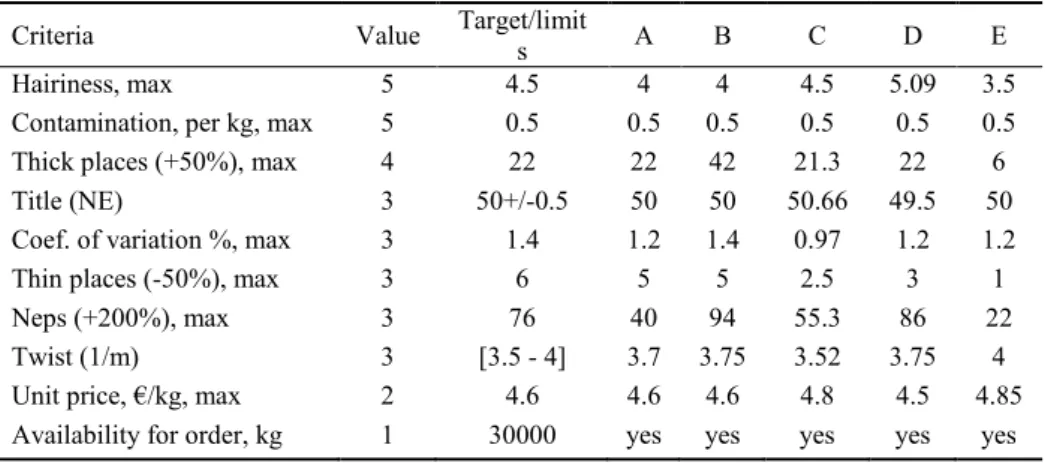
Criteria involved, target/upper values and data for supply alternatives A, B, C, D and E (i.e., performance of alternative i in criteria j, sij) are shown in Table 1, as
formulated by the decision makers. The relative importance of criteria is expressed in a scale from “5” to “1”, i.e. from the most to least important.
Table 1. Dataset on criteria, target/limit levels and matrix of alternatives, as initially formulated
Criteria Value Target/limits A B C D E
Hairiness, max 5 4.5 4 4 4.5 5.09 3.5
Contamination, per kg, max 5 0.5 0.5 0.5 0.5 0.5 0.5
Thick places (+50%), max 4 22 22 42 21.3 22 6
Title (NE) 3 50+/-0.5 50 50 50.66 49.5 50
Coef. of variation %, max 3 1.4 1.2 1.4 0.97 1.2 1.2
Thin places (-50%), max 3 6 5 5 2.5 3 1
Neps (+200%), max 3 76 40 94 55.3 86 22
Twist (1/m) 3 [3.5 - 4] 3.7 3.75 3.52 3.75 4
Unit price, €/kg, max 2 4.6 4.6 4.6 4.8 4.5 4.85 Availability for order, kg 1 30000 yes yes yes yes yes
Some important conclusions were made in this preliminary stage through analyses and discussion with decision-makers. All criteria were quantitative, measured in different scales (or indexes); all data was treated deterministically, with possibility to carry out laboratorial samples quality testing. In this particular case it was decided to order from only one source, to guarantee the lot´s homogeneity.
Contamination criterion is redundant for this particular case, but should not be excluded. Availability criterion must be transformed in capacity constraint; in this case any supplier must have capacity equal to or greater than monthly (and total) demand, to be considered as a valid alternative for the final stage.
For the remaining criteria minimizing is the sense of optimization, i.e. “less is better”, with exception of two side criteria where “exact is better”. These dual-side criteria are Title (NE) and Twist. Twist criterion seems like interval of acceptance (as initially formulated), but it is really dual-side target value. The value of 3.8 was defined as target, with values of 3.5 and 4.0 as rejection thresholds. In such cases a sum of dual-side deviations should be minimized.
There is one important issue related with target values: only one of the 5 alternatives, chosen for final analysis, actually fulfils all limits - supplier A. Consequently, the nature of the target/upper limits is not clear: are they rejection or aspiration thresholds? To simplify the final selection, compensatory decision rule should be employed in that stage. Thus, all alternatives out of the feasible area must be excluded by defined rejection thresholds (veto levels) on respective criteria.
3.2 Weighted score model
Weighted score models are widely used by professionals, being a common model recommended in procurement and supply chain management manuals [10]. It is worth mentioning that this tool is familiar for decision makers and is normally used by the Group in suppliers’ performance evaluation.
A sum of the scores of a supplier multiplied by relative weights of each criteria, gives a total score of the supplier. Possible subjectivity in defining criteria weights [11] and proper scaling of criteria values are known difficulties for the implementation of simple weighted models.
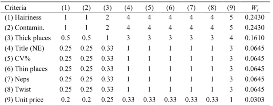
In order to define criteria relative weights objectively, analytic hierarchy process (AHP) was used. This well-known decision-making heuristic, based on pairwise comparisons, was introduced by Saaty in 1981 [12]. Thus, criteria were compared to each other in a 1 to 9 scale, with 1 meaning “equally important” and 9 meaning “extremely more important”. The resulting pairwise comparison matrix and relative weights of criteria (Wj) are presented in Table 2.
Table 2. Calculation of criteria relative weights with AHP
Criteria (1) (2) (3) (4) (5) (6) (7) (8) (9) Wj (1) Hairiness 1 1 2 4 4 4 4 4 5 0.2430 (2) Contamin. 1 1 2 4 4 4 4 4 5 0.2430 (3) Thick places 0.5 0.5 1 3 3 3 3 3 4 0.1610 (4) Title (NE) 0.25 0.25 0.33 1 1 1 1 1 3 0.0645 (5) CV% 0.25 0.25 0.33 1 1 1 1 1 3 0.0645 (6) Thin places 0.25 0.25 0.33 1 1 1 1 1 3 0.0645 (7) Neps 0.25 0.25 0.33 1 1 1 1 1 3 0.0645 (8) Twist 0.25 0.25 0.33 1 1 1 1 1 3 0.0645 (9) Unit price 0.2 0.2 0.25 0.33 0.33 0.33 0.33 0.33 1 0.0303
Decision makers showed preference in developing the models in the familiar Excel spreadsheet interface to avoid investment of time and money in software in this experimental stage. Consistency ratio was calculated in the same Excel form and was equal to 0.014; the calculation was repeated in BeSmart2 free software [13], with the same result. It means that the matrix is almost consistent, apparently due to the initial criteria ordering.
The criteria weights obtained were considered realistic by decision makers, being necessary to explore the low weight of Price criterion. There were discussed two complementary explanations. Firstly, some lot of yarn, which doesn´t meet upper limits of the technical specifications, has drastically diminished its value. The second explanation concerns the decision makers´ knowledge that price might vary more or less 10% around the target value. Hence, Price criterion was “undervalued” because price is expected to fluctuate within known and limited interval.
In order to solve the scaling problem, the following linear normalization procedure was applied to 7 criteria (one-side) of minimization type:
rij = min{sij}/sij (1)
Where sij is an actual value of alternative i on criterion j, rij is a score of alternative
i on criterion j, with i = 1, 2, …, m, j = 1, 2, …, n, being m the number of alternatives and n the number of criteria. Alternative(s) with the lowest value, on a particular criterion, will be scored as equal to “1”, other alternatives will be scored proportionally less than “1” (for maximization the inverse should be used).
For two dual-side criteria, decision-makers suggested to divide the range of acceptable values in intervals with declining utility function. Mathematically, it is the same as the calculation of the membership function of triangular fuzzy numbers, as described in [14]. Having alternative(s) matching the exact target value, data will be already normalized in the same sense as in equation (1), otherwise the inverse of (1) is applied.
In the process of analyzing different normalization schemes, attention was drown to the question of the distinction between rejection and aspiration levels on criteria. Rescreening performed, decision makers decided to drop the supplier B, which exceeds largely rejection thresholds on Thick places and Neps. Supplier E, which does not meet Price criterion, was kept in analyses, being price a mere target value. Options C and D are kept; zero score will be assigned to alternatives on criteria where original limits are matched or exceeded. For Thin places criterion the indifference level of “3” was established.
With the purpose to demonstrate sensitivity analysis, the relative criteria weights were recalculated with Simple multi-attribute rating technique (SMART), as described in [13]. Having significant differences between relative weights obtained with AHP and SMART, AHP criteria weights were hold up as more realistic ones.
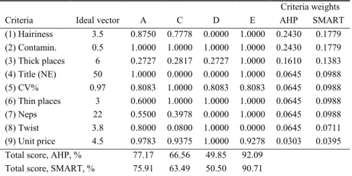
Normalized data, two types of criteria weights and final total scores of suppliers are shown in Table 3. Total scores of alternatives in percentage display the proximity to the ideal solution, in accordance with the preference set of the decision-makers.
Supplier D, the cheapest one, is clearly a dominated option; supplier E, the most expensive one, is considered as the best alternative. Supplier A, the only one which does not violate initial target/upper limits, is the second best alternative. Different relative criteria weights have no significant impact on total score of suppliers. The
way in which the data was structured and visualized was innovative to the decision makers, but final scores of suppliers are consistent with their experience.
Table 3. Weighted score model
Criteria weights
Criteria Ideal vector A C D E AHP SMART
(1) Hairiness 3.5 0.8750 0.7778 0.0000 1.0000 0.2430 0.1779 (2) Contamin. 0.5 1.0000 1.0000 1.0000 1.0000 0.2430 0.1779 (3) Thick places 6 0.2727 0.2817 0.2727 1.0000 0.1610 0.1383 (4) Title (NE) 50 1.0000 0.0000 0.0000 1.0000 0.0645 0.0988 (5) CV% 0.97 0.8083 1.0000 0.8083 0.8083 0.0645 0.0988 (6) Thin places 3 0.6000 1.0000 1.0000 1.0000 0.0645 0.0988 (7) Neps 22 0.5500 0.3978 0.0000 1.0000 0.0645 0.0988 (8) Twist 3.8 0.8000 0.0800 1.0000 0.0000 0.0645 0.0711 (9) Unit price 4.5 0.9783 0.9375 1.0000 0.9278 0.0303 0.0395 Total score, AHP, % 77.17 66.56 49.85 92.09
Total score, SMART, % 75.91 63.49 50.50 90.71
3.3 Goal programming model
Dropped one source strategy, in this or future buying decisions, the weighted score model will be of little use. If individual suppliers´ capacities meet total of demand, the final choice will be the same – to assign the whole order to the “best” alternative. But will it be the most efficient solution? Mathematical programming models are indicated in such decision situations as multiple-source, multiple-product and multiple-period decisions, with lot-sizing problem and possible price discounts [15].
Goal programming is one of the main approaches for the supplier selection problem [5]. With expressed underlying philosophy of satisfying multiple objectives and without evidence of different priorities levels, weighted goal programming model was chosen.
Model indices, parameters and decision variables are stated as follows: i set of suppliers, i {1, …, 4}
j set of criteria, j {1, …, 9} kj set of goals to achieve on criteria j
sij performance of supplier i on criterion j
d buyer´s demand ci supplier´s i capacity
wj relative weights of criteria j, assigned by the decision makers
xi decision variable of order quantity, allocated to supplier i
nj underachievement deviational variable on criterion j
pj overachievement deviational variable on criterion j
min a = w1p1/k1 + w2p2/k2 + w3p3/k3 + w4(n4 + p4)/k4 + w5p5/k5 + w6p6/k6 + w7p7/k7 + w8(n8 + p8)/k8 + w9p9/k9 (2) Subject to: ∑ xi = d, i {1, …, 4} (3) ci ≥ d, i {1, …, 4} (4) ∑ xisij + nj – pj = kj, i {1, …, 4},j {1, …, 9} (5) nj, pj≥ 0, j {1, …, 9} (6) xi≥ 0 and binary, i {1, …, 4} (7)
The formulation allows minimization of deviations from stated goals on 9 criteria: deviational variables are multiplied by the weighting vector wj of criteria importance
(given by Table 2) and divided by the set kj of targets on criteria to obtain normalized
unites [14]. Performance data of supplier i on criterion j, sij, is given in the Table 1.
The problem solution was obtained using Solver from Excel and a set of experiences was performed to familiarize decision makers with the mathematical programming.
With initial set of targets/limits used as first set of goals, the solution was to order to the supplier A. The solution is consistent with the fact that supplier A is the unique one which does not violate the initial set of targets. But such result is based on pessimistic setting of targets.
Switching to more rigorous set of targets (4, 0.5, 22, 50, 1.2, 3, 55.3, 3.8, 4.6) or to the ideal vector as set of targets, the solution is to order to supplier E, which is consistent with the output of the weighted score model. Only two criteria, Switch and Price were not completely satisfied.
The next step was relaxing of capacity restriction (4) and of the binary condition of decision variables xi (7), with the same target setting. The solution found was to split
the order between all suppliers in the following proportions: A: 0.399, C: 0.102, D: 0.125 and E: 0.374. Thus, the achievement function value decreased 7.47 times, with total cost of solution reduced from 145500€ to 141043€ (less 3.06%). Only the price criterion was slightly overachieved.
In this way, two different policy scenarios (one- and multiple-sourcing strategies) and “supplier A” scenario might be visualized and compared, with sensitivity analysis facilitated, providing an analysis tool for the decision makers.
Such factors as familiar Excel interface, and known, important but not very complex decision process, were crucial to draw attention and genuine interest of decision makers to the approach based on mathematical programming. With such experience it will be easier to assure openness and acceptance of more complex decision modelling with integer variables, additional policy and systems constraints.
3.4 Analytic hierarchy process model
In the final stage of the case it was commented by the decision makers that Title (NE) dual-side criterion might be seen as asymmetric. It is a density index - yarn lot with
less than 50 is thicker, provoking major consumption. Thinner lots, with Title (NE) more than 50, also have diminished value, but without consumption problem. Therefore, the utility function on this criterion might be seen as linearly decreasing to the left of the target level, and non-linearly to the right.
This specific issue was not seen as very relevant, but the pertinent question of an appropriate technique to introduce the concept of non-linearity was emerged. Already used, AHP technique is a decision making heuristic, able to aggregate tangibles and intangibles factors and non-linearity [11]. The AHP model with three levels was elaborated: supplier selection level, criteria level and alternatives level.
The vector of relative weights of criteria was already calculated for the previous models, as shown in Table 2. Comparisons on one-side criteria were based on numerical data, with no need to calculate consistency ratios. Performance of alternatives on dual-side criteria was assessed on a 1 to 9 scale, with asymmetry of Title (NE) criterion taken into account; consistency ratios on Title (NE) and Twist criteria were 0.00599 and 0.00597 respectively. Resulting data of AHP model is shown in Table 4.
Table 4. Final AHP evaluation matrix
Criteria Weights A C D E (1) Hairiness 0.2430 0.2619 0.2328 0.2059 0.2994 (2) Contamination 0.2430 0.2500 0.2500 0.2500 0.2500 (3) Thick places 0.1610 0.1493 0.1542 0.1493 0.5473 (4) Title (NE) 0.0645 0.4251 0.0938 0.0561 0.4251 (5) CV% 0.0645 0.2360 0.2920 0.2360 0.2360 (6) Thin places 0.0645 0.1034 0.2069 0.1724 0.5172 (7) Neps 0.0645 0.2496 0.1805 0.1161 0.4538 (8) Twist 0.0645 0.3221 0.0704 0.5371 0.0704 (9) Unit price 0.0303 0.2545 0.2439 0.2602 0.2414 Total weights of suppliers on criteria 0.242 0.204 0.215 0.339 Scores of suppliers on criteria, % 71.54 60.20 63.40 100.00 Recognized as realistic and consistent, the output of AHP model differs from the one of weighted score model: suppliers E and A are maintained as best alternatives, but suppliers C and D switched their ranking position. This score differences are consequent of the fact that AHP model maintains intrinsic values of alternatives on criteria even when upper limits are matched or surpassed. One more time it highlights the importance of a clear definition of rejection levels on the screening, pre-selection stage of the supplier selection problem.
With 11 tables designed, the process of modelling was not really difficult or work intensive, but using of decision-support software, such as Be Smart2, makes the process more fluent. With rejection levels, nature of data and of utility function defined, the use of AHP model to evaluate and select suppliers was seen as an approach very intuitive, objective and universal. AHP was considered as an excellent
initial decision-making technique; also it’s potential to make part of integrated approaches and to provide input data for mathematical programming was commented.
4 Evaluation and feedback of the decision makers
A final interview was dedicated to the feedback and analyses of perceived value by the decision makers. The framework for decision makers´ evaluation and validation, developed by Boer and Van der Wegen [1], served as a base for this interview.
It was found that modelling of the real purchasing decision was performed properly, matching the decision situation in 90-95%. Some criteria, considered unimportant, were excluded from the final decision process by the decision makers, but all available information was incorporated, inclusively opinions and experience. Capacity of the decision models to structure, facilitate and enhance internal and external communication was strongly recognized. Models elaborated were seen as flexible to include new aspects of the problem and to be extended or used in a different context.
The process of structuring and visualization of the supplier selection problem was found practically useful, giving mathematical tools to analyze multiple criteria, especially USTER® parameters, in the aggregated manner. Previously the process was more experience-based, subjective and qualitative, without aggregation approach. The real output of the supplier selection was to order from the supplier A, the second best alternative. The supplier E was seen as the best alternative but only with declared level on Thick places criterion confirmed in laboratory. Tests performed accused higher levels on this criterion, though the supplier E was dropped. All three models defined these two suppliers as the best options, the decision modelling outcome was considered acceptable and consistent with the decision makers´ experience.
Elaboration of such decision support models had no direct monetary costs; cognitive efforts and time investment were considered justified, bringing new skills and insights to the decision making process.
Such concepts as rejection levels, compensatory decision rule, quantitative and qualitative data, sensitivity analysis, non-linearity and asymmetry were seen as valuable contributes to practical decision making skills of managers. Albeit the problem of yarn supplier selection is well-known for the decision-makers, decision modelling process actually brought some new knowledge and angles of it. In long-term perspective, the interest to keep implementation of MCDA techniques in the procurement practice was firmly assumed by the decision makers.
5 Conclusions
The process of decision modelling with analysis of relevant criteria and of rejection/aspiration levels, criteria weights calculation, normalization procedures and goal programming formulation, was considered as benefic to the deep understanding of the decision problem. Structured, aggregated and visualized data enforces analysis
and facilitates objective final choice decision. Approaches applied have demonstrated potential to be extended within and out of the context of the supplier selection problem.
The research trend of more and more complex theoretical modelling of the supplier selection decisions may not be beneficial for the problem of practical implementation. Modelling a typical and important, but not very complex, decision process with some basic MCDA techniques was crucial to capture attention of managers and to gain synergies. Positive experience with realistic and useful outputs, acquired knowledge and skills of the decision makers (the capacity to analyze a decision problem and the ability to apply different approaches) showed to be the important elements for the successful implementation of MCDA by procurement professionals.
Acknowledgment. This work has been supported by FCT - Fundação para a Ciência e Tecnologia in the scope of the PEst-UID/CEC/00319/2013.
References
1. De Boer, L., Van Der Wegen, L. L. M.: Practice and promise of formal supplier selection: A study of four empirical cases. J. Purch. Supply Manag. 9(3), 109–118 (2003)
2. De Boer, L., Labro, E., Morlacchi, P.: A review of methods supporting supplier selection. Eur. J. Purch. Supply Manag. 7(2), 75–89 (2001)
3. Bruno, G., Esposito, E., Genovese, A., Passaro, R.: AHP-based approaches for supplier evaluation: Problems and perspectives. J. Purch. Supply Manag. 18(3), 159–172 (2012) 4. Jadidi, O., Zolfaghari, S., Cavalieri, S.: A new normalized goal programming model for
multi-objective problems: A case of supplier selection and order allocation. Int. J. Prod. Econ. 148, 158–165 (2014)
5. Ho, W., Xu, X., Dey, P.K.: Multi-criteria decision making approaches for supplier evaluation and selection: A literature review. Eur. J. Oper. Res. 202(1), 16–24 (2010) 6. Chai, J., Liu, J.N.K., Ngai, E.W.T.: Application of decision-making techniques in supplier
selection: A systematic review of literature. Expert Syst. Appl. 40(10), 3872–3885 (2013) 7. Arnott, D., Pervan, G.: Eight key issues for the decision support systems discipline. Decis.
Support Syst. 44(3), 657–672 (2008)
8. Gibbert, M., Ruigrok, W., Wicki, B.: What passes as a rigorous case study? Strateg. Manag. J. 29(13), 1465–1474 (2008)
9. Uster Technologies, http://www.uster.com
10. Monczka, R.M., Handfield, R.B., Giunipero, L.C., Patterson, J.L.: Purchasing and Supply Chain Management, 4th edition.South-Western Cengage Learning, Mason (2009)
11. Ghodsypour, S.H., O’Brien, C.: A decision support system for supplier selection using an integrated analytic hierarchy process and linear programming. Int. J. Prod. Econ. 56/57, 199–212 (1998)
12. Figueira, J., Greco, S., Ehrgott, M.: Multiple Criteria Decision Analysis: State of the Art Surveys. Springer Science + Business Media Inc., New York (2005)
13. Tereso, A., Amorim, J.: BeSmart2: A Multicriteria Decision Aid Application. New Contributions in Information Systems and Technologies, in Advances in Intelligent Systems and Computing, vol. 353, pp. 701–710. Springer International Publishing (2015)
14. Jones, D., Tamiz, M.: Practical Goal Programming. Springer US, Boston (2010)
15. Aissaoui, N., Haouari, M., Hassini, E.: Supplier selection and order lot sizing modeling: A review. Comput. Oper. Res. 34(12), 3516–3540 (2007)