EJASA, Electron. J. App. Stat. Anal.
http://siba-ese.unisalento.it/index.php/ejasa/index
e-ISSN: 2070-5948
DOI: 10.1285/i20705948v7n2p228
Reliability estimation of k-unit series system based on progressively censored data
By Potdar K.G., Shirke D.T.
Published: 14 October 2014
This work is copyrighted by Universit`a del Salento, and is licensed un-der aCreative Commons Attribuzione - Non commerciale - Non opere derivate 3.0 Italia License.
For more information see:
Vol. 07, Issue 02, 2014, 228-253 DOI: 10.1285/i20705948v7n2p228
Reliability estimation of k-unit series
system based on progressively censored
data
K. G. Potdar
∗aand D. T. Shirke
baDepartment of Statistics, Ajara Mahavidyalaya, Ajara, DistKolhapur, Maharashtra, India -416505.
bDepartment of Statistics, Shivaji University, Kolhapur, DistKolhapur, Maharashtra, India -416004.
Published: 14 October 2014
In this article, we consider a k-unit series system with component lifetime distribution to be a member of the scale family of distributions. We discuss estimation of the scale parameter and estimation of reliability function of the family based on progressively Type-II censored sample. The maximum like-lihood estimator (MLE) of the scale parameter is derived using Expectation-Maximization (EM) algorithm and is used to estimate reliability function. Confidence intervals are constructed using asymptotic distribution of MLE. β -expectation tolerance interval for lifetime of the system is obtained. We consider half-logistic distribution as a member of the scale family and study performance of the MLE, reliability estimate and confidence interval using simulation experiments. Illustration through real data example is provided. keywords: Progressively Type-II censoring, EM algorithm, MLE, confi-dence interval, coverage probability, reliability, β-expectation tolerance in-terval, half-logistic distribution.
1 Introduction
In industrial phenomenon series systems are widely used. Electric, automobile as well as in chemical industry various units are connected in series. Here system is working if all
∗
Corresponding author: [email protected].
c
Universit`a del Salento ISSN: 2070-5948
units in system are working. If any one unit is failed then system fails. Thus, system life is smaller than unit life. Life testing under series system is more costly, because failure of one unit reflects in system failure. Therefore, we use censoring criteria, in that; we remove some working systems without observing its failure time. The unobserved failure time data are called censored data.
Broadly censoring is classified into two types; Type-I and Type-II censoring. Type-I censoring depends on time. In this type, an experiment continues up to a pre-determined timeT. Units having failure time after timeT are not observed. Here, failure time will be known exactly only if it is less than T. For example, if n units are placed on test, but decision is made to terminate the test at time T, then failure times will be known exactly only for those units that fail before timeT. In Type-I censoring, the number of exact failure times observed is random.
Type-II censoring scheme is often used in life testing experiment. In this scheme only m units in a random sample of size n(m < n) are observed. Progressive Type-II censoring is a generalization of Type-II censoring. In progressive censoring scheme, the number m andR1,R2,...., Rm are fixed prior to the test and Pmi=1Ri =n−m. At the
first failure R1 units are randomly removed from remaining n−1 units. At the second failure,R2 units are randomly removed from remaining n−2−R1 units and so on. At the mth failure all remaining Rm units are removed. Here, we observe failure time of
m units and remaining n−m units are removed at different stages of experiment. In conventional Type-II censoring schemeR1=R2 =....=Rm−1= 0 andRm =n−m. In
this article, the progressive Type-II censoring scheme is considered.
Many authors studied progressive Type-II censoring scheme for various lifetime dis-tributions. Cohen (1963) introduced progressive Type-II censoring. Mann (1969) and Mann (1971) considered Weibull distribution with progressive censoring. Balakrish-nan and Asgharzadeh (2005), BalakrishBalakrish-nan et al. (2003) and BalakrishBalakrish-nan et al. (2004) discussed inference for half-logistic, Gaussian and extreme value distribution under pro-gressive Type-II censoring scheme respectively. Ng (2005) studied parameter estimation for modified Weibull distribution under progressive Type-II censoring. Balakrishnan and Aggarwala (2000) gave details about progressive censoring. Balakrishnan (2007) studied various distributions and inferential methods for progressively censored data. Pradhan (2007) considered point and interval estimation of a k-unit parallel system based on progressive Type-II censoring scheme with exponential distribution as the component life distribution.
Kim and Han (2010) discussed half-logistic distribution for Type-II progressively censored samples. Iliopoulos and Balakrishnan (2011) studied likelihood inference for Laplace distribution based on progressively Type-II censored samples. Asgharzadeh and Valiollahi (2011) considered estimation of the scale parameter of the Lomax distribution under progressive censoring scheme. Krishna and Malik (2012), Krishna and Kumar (2011) and Krishna and Kumar (2013) studied reliability estimation in Maxwell, Lind-ley and generalized inverted exponential distribution with progressively Type-II censored data. Recently, Potdar and Shirke (2014) discussed inference for the scale parameter of lifetime distribution of k-unit parallel system based on progressively Type-II censored data. Potdar and Shirke (2012) studied inference for the distribution of a k-unit
par-allel system with exponential distribution as the component life distribution based on Type-II progressively censored sample. Potdar and Shirke (2013a) discussed inference for the parameters of generalized inverted family of distributions. Potdar and Shirke (2013b) studied reliability estimation for the distribution of a k-unit parallel system when Rayleigh distribution as component lifetime distribution.
Dempster et al. (1977) introduced expectation-maximization (EM) algorithm. They presented maximum likelihood estimation for incomplete data. McLachlan and Krishnan (2007) gave more details about EM algorithm. Little and Rubin (2002) have discussed EM algorithm for exponential family of distributions. Pradhan and Kundu (2009) used EM algorithm to estimate parameters of generalized exponential distribution under pro-gressive Type-II censoring scheme. Ng et al. (2002) used EM algorithm to estimate parameters of lognormal and Weibull distributions under Type-II censoring scheme. In this article, we use EM algorithm for estimation of the parameters of a k-unit series system based on progressive Type-II censoring scheme when unit lifetime distribution belongs to the scale family. Parameter estimation is based on the lifetimes of the system. We assume that n units are put on test and failure times of Pm
i=1Ri = n−m. units
are censored. Failure times of these censored units are unknown. We consider this data as missing and use EM algorithm to compute MLE. We use idea of missing information principle of Louis (1982). Asymptotic normal distribution of MLE is used to construct confidence interval for the scale parameter. We also discuss tolerance interval for the lifetime of the system, on the lines of Kumbhar and Shirke (2004).
The present work is different than the work reported by Pradhan (2007) in many aspects. The first thing is that we consider scale family of distributions and exponential distribution considered by Pradhan (2007) is a member of the family. Further, we obtain MLE using EM algorithm instead of using Raphson method. We use Newton-Raphson method within EM algorithm. Pradhan (2007) has considered only parameter estimation, while we consider inference of parameter as well as reliability function. We use missing information principle to compute Fisher information. We illustrate use of the results developed with half-logistic distribution, which is a member of scale family. Number of schemes that we consider are 30, which include schemes with small sample sizes.
In Section 2, we introduce the model and obtain MLE for the scale parameter and reliability function. We also provide an expression for Fisher information. Asymptotic confidence interval for the scale parameter based on MLE, log-MLE and confidence in-terval for the reliability function is discussed in the same section. Section 3 provides β-expectation tolerance interval for the lifetime of a k-unit series system based on pro-gressively censored data. In Section 4, we consider the half-logistic distribution as a member of the scale family and discuss MLE, reliability function, confidence intervals and tolerance intervals. Performance of the MLE and confidence intervals of scale param-eter and reliability function of half-logistic distribution is investigated using simulations. Results of simulation study have been reported in Section 5. Real data application is discussed in Section 6. Conclusions are presented in Section 7.
2 Model and Estimation of the Scale Parameter
Let Gλ be a scale family of lifetime distributions where λ is the parameter of the
in-terest. Consider a k-unit series system with independent and identically distributed units having lifetimes X1, X2, ...., Xk of k units. That is, Xi is the lifetime of the ith
unit having cumulative distribution function (cdf) G xi
λ
. The lifetime of the system is X=M in.(X1, X2, ...., Xk). The cdf ofX is F(x;λ) = 1−h1−G x λ ik x≥0, λ >0. The probability density function (pdf) of X is
f(x;λ) = k λg x λ h 1−G x λ ik−1 x≥0, λ >0. whereg(.) is the pdf ofXi when λ= 1.
2.1 Maximum Likelihood Estimation
Supposenk-unit series systems are under test and we observe failure times ofmsystems under progressive type-II censoring. Let (R1, R2, ...., Rm) be a progressive censoring
scheme.
The likelihood function for the observed data is L(λ|x) =C m Y i=1 f(x(i);λ) 1−F(x(i);λ)Ri , where C=n m−1 Y j=1 n−j− j X i=1 Ri ! . L(λ|x) =C m Y i=1 k λg x(i) λ h 1−Gx(i) λ ik−1h 1−Gx(i) λ ikRi ,
Suppose x1, x2, ...., xm is the observed data and z1, z2, ...., zm is the censored data. We
note thatzi is a vector withRi elements, which is not observable fori= 1,2, ...., m. The
censored data Z = (z1, z2, ...., zm) can be considered as missing data.
X = (x1, x2, ...., xm) is observed data. W = (X, Z) is the complete data set. Then
complete log-likelihood function is
Lc=nlog(k)−nlog(λ) + m X i=1 log h g xi λ i + (k−1) m X i=1 log h 1−G xi λ i + m X i=1 Ri X j=1 log h g zij λ i + (k−1) m X i=1 Ri X j=1 log h 1−G zij λ i . (1)
In order to obtain MLE of λ, we use EM algorithm due to Dempster et al. (1977). For the E step in EM algorithm we take Expectation of Zij. The derivative of Lc with
respect toλis taken for the M step, where dLc dλ =− n λ − 1 λ2 m X i=1 xig0 xλi g xi λ + (k−1) λ2 m X i=1 xiG0 xλi 1−G xi λ − 1 λ2 m X i=1 Ria(xi, k, λ0) + (k−1) λ2 m X i=1 Rib(xi, k, λ0). (2) where a(xi, k, λ) =E Zijg0 Z ij λ g Z ij λ Zij > xi = ∞ Z xi zg0 λz g λz f(z;λ) 1−F(xi;λ) dz, and b(xi, k, λ) =E ZijG0 Z ij λ 1−G Z ij λ Zij > xi = ∞ Z xi zG0 λz 1−G λz f(z;λ) 1−F(xi;λ) dz.
We have to solve equation dLc
dλ = 0 to obtain λ1 as the solution. But this equation does
not have solution in the closed form. Therefore we use Newton-Raphson method and compute λ1. By using λ1, we compute a(xi, k, λ1) and b(xi, k, λ1). This ends M-step.
We continue this procedure until convergence takes place.
In Newton-Raphson method, we have to choose initial value ofλ. We use least square estimate. Ng (2005) discussed estimation of model parameters of modified Weibull dis-tribution based on progressively Type-II censored data where the empirical disdis-tribution function is computed as (see Meeker and Escobar (1998))
ˆ F(xi) = 1− i Y j=1 (1−pˆj), with ˆ pj = 1 n−Pj k=2Rk−1−j+ 1 forj= 1,2, ..., m.
The estimate of the parameter can be obtained by using least square fit of simple linear regression. yi =βxi with β= 1 λ yi=G−1 1− h 1−Fˆ(xi−1) i1/k +h1−Fˆ(xi) i1/k 2 fori= 1,2, ..., m. ˆ F(x0) = 0,
The least square estimates ofλis given by ˆ λ0 = Pm i=1x2i Pm i=1xi yi ,
We use ˆλ0 as an initial value of λ to obtain the MLE ˆλn using Newton-Raphson
method. Reliability function at time t is R(t) = 1−G t λ k t≥0, λ >0.
The Maximum likelihood estimator ofR(t) is ˆ Rn(t) = 1−G t ˆ λn k t≥0. 2.2 Fisher Information
We compute observed Fisher information using the idea of missing information principle of Louis (1982).
Thus, observed information = complete information - missing information. Ix(λ) =Iw(λ)−Iw|x(λ),
where the complete information =Iw(λ) =−E
h
d2L
dλ2
i
and L is the log-likelihood function based on allnobservations. We obtain Iw(λ) and Iw|x(λ) in the following.
Now, L=nlog(k)−nlog(λ) + n X i=1 log h g xi λ i + (k−1) n X i=1 log h 1−G xi λ i . (3) and dL dλ =− n λ− 1 λ2 n X i=1 xig0 xλi g xi λ + (k−1) λ2 n X i=1 xiG0 xλi 1−G xi λ . d2L dλ2 = n λ2+ 1 λ4 n X i=1 x2ig xi λ g00 xi λ −x2i g0 xi λ 2 + 2λxig xλi g0 xi λ g xi λ 2 −(k−1) λ4 n X i=1 x2i 1−G xi λ G00 xi λ +x2i G0 xi λ 2 + 2λxi 1−G xi λ G0 xi λ 1−G xi λ 2 .
Complete information is given by Iw(λ) =− n λ2 − 1 λ4 n X i=1 E Xi2gXi λ g00Xi λ −Xi2hg0Xi λ i2 + 2λXig Xi λ g0Xi λ h gXi λ i2 +(k−1) λ4 n X i=1 E Xi2h1−GXi λ i G00Xi λ +Xi2hG0Xi λ i2 + 2λXi h 1−GXi λ i G0Xi λ h 1−GXi λ i2 . (4) Missing information is given by
Iw|x(λ) = m X i=1 RiIw(i|)x(λ) =− m X i=1 Ri X j=1 EZ|X d2log(f(Zij|xi, λ)) dλ2 Consider fZ|X(zij|xi, λ) = f(zij;λ) 1−F(xi, λ) = k λg zij λ 1−G zij λ k−1 1−G xi λ k . Therefore,
log(f) =log(k)−log(λ) +log
h g zij λ i + (k−1)log h 1−G zij λ i −klog h 1−G xi λ i . dlogf dλ =− 1 λ− zijg0 zλij λ2g zij λ + (k−1)zijG0 zλij λ2 1−G zij λ − kxiG0 xλi λ2 1−G xi λ . and d2logf dλ2 = 1 λ2 + z2ijg zij λ g00 zij λ −zij2 g0 zij λ 2 + 2λzijg zλij g0 zij λ λ4 g zij λ 2 − (k−1) n zij2 1−G zij λ G00 zij λ +z2ijG0 zij λ 2 + 2λzij 1−G zij λ G0 zij λ o λ4 1−G zij λ 2 + k n x2i 1−G xi λ G00 xi λ +x2i G0 xi λ 2 + 2λxiG0 xλi 1−G xλi o λ4 1−G xi λ 2 .
Hence, missing information is
Iw|x(λ) = m X i=1 RiIw(i|)x(λ) =− m X i=1 Ri X j=1 EZ|X d2log(f(Zij|xi, λ)) dλ2
=−n−m λ2 −1 λ4 m X i=1 Ri X j=1 E Z2 ijg Z ij λ g00Zij λ −Z2 ij h g0Zij λ i2 + 2λZijg Z ij λ g0Zij λ h gZij λ i2 −(k−1) λ4 m X i=1 Ri X j=1 E Zij2 h1−GZij λ i G00Zij λ +Zij2 hG0Zij λ i2 h 1−GZij λ i2 −2(k−1) λ3 m X i=1 Ri X j=1 E Zij h 1−GZij λ i G0Zij λ h 1−GZij λ i2 +k λ4 m X i=1 Ri " x2i 1−G xi λ G00 xi λ +x2i G0 xi λ 2 + 2λxiG0 xλi 1−G xλi 1−G xi λ 2 # . (5) Using expressions in equations (4) and (5) we obtain observed Fisher information.
2.3 Confidence Intervals
By using asymptotic normal distribution of MLE ˆλn, we construct confidence interval
for λ. Let ˆσ2( ˆλ
n) = I( ˆλ1
n) is the estimated variance of ˆλn. Therefore, 100(1
−α)% asymptotic confidence interval forλis given by
ˆ λn−τα/2 q ˆ σ2(ˆλ n), λˆn+τα/2 q ˆ σ2(ˆλ n) , (6)
whereτα/2 is the upper 100(α/2)th percentile of standard normal distribution.
Meeker and Escobar (1998) reported that the asymptotic confidence interval forλcan be computed usinglog(ˆλn). An approximate 100(1−α)% confidence interval forlog(λ)
is given by log(ˆλn)−τα/2 q ˆ σ2(log(ˆλ n)), log(ˆλn) +τα/2 q ˆ σ2(log(ˆλ n)) ,
where ˆσ2(log( ˆλn)) is the estimated variance of log(ˆλn) which is approximated by
ˆ σ2(log( ˆλn)) ≈ σˆ 2( ˆλ n) ˆ λn
2 . Hence, an approximate 100(1−α)% confidence interval for λ
is given by ˆ λne −τα/2 √ ˆ σ2(ˆλn) ˆ λn ! , λˆne τα/2 √ ˆ σ2(ˆλn) ˆ λn ! . (7)
Let ˆRnis the MLE of reliability functionR(t) andσ2( ˆRn) is the variance of ˆRn, where ˆ σ2( ˆRn)≈ k 2t2 ˆ λ4 n 1−G t ˆ λn 2(k−1) G0 t ˆ λn 2 ˆ σ2(ˆλn)
Therefore, 100(1−α)% asymptotic confidence interval for R(t) is given by
ˆ Rn−τα/2 q ˆ σ2( ˆR n), Rˆn+τα/2 q ˆ σ2( ˆR n) , (8)
3 Tolerance Intervals
Kumbhar and Shirke (2004) derived the expression for β-expectation tolerance interval for the lifetime distribution of a k-unit parallel system with component life as expo-nential distribution. They investigated the performance of the tolerance interval based on complete data. We study the performance of the tolerance interval for the lifetime distribution of a k-unit series system based on progressively Type-II censored data for the scale family of distributions. Let lβ(λ) be the lower quantile of order β of the cdf
F(x;λ). Then, we have lβ(λ) =λG−1 h 1−(1−β)1/k i .
Thus, an upper β-expectation tolerance interval for F(x;λ) is obtained by Iβ = (0, lβ(λ)).
The maximum likelihood estimator oflβ(λ) is given by
lβ(ˆλn) = ˆλnG−1
h
1−(1−β)1/k
i
, yielding an approximate β- expectation tolerance interval as
ˆ Iβ = 0, lβ(ˆλn) .
The expectation of ˆIβ can be obtained approximately using the approach suggested by
Atwood (1984) and given as,
E h F(Iβ(ˆλn);λ) i ≈β−0.5F02σ2(ˆλn) + F01σ2(ˆλn)F11 F10 , (9) where F10= dF dx, F01= dF dλ, F11= d2F dxdλ, F02= d2F dλ2, F10= k λ h 1−Gx λ ik−1 gx λ , F01=− kx λ2 h 1−Gx λ ik−1 G0x λ , F11=− k λ3 h 1−Gx λ ik−2 ×
n xh1−Gx λ i g0x λ +x(k−1)G0x λ gx λ +λh1−Gx λ i gx λ o , F02= kx λ4 h 1−Gx λ ik−2 × xh1−Gx λ i G00x λ −x(k−1)hG0x λ i2 + 2λh1−Gx λ i G0x λ . The derivatives ofF are evaluated atx=lβ(λ) withλ= ˆλn. Instead of the actual value
of σ2(ˆλn) we use estimate of it.
4 Application to Half-Logistic Distribution
Consider a member of the scale family of distributions, namely half-logistic distribution with scale parameter λ. The cdf of X is
F(x;λ) = 1− " 2e−x/λ 1 +e−x/λ #k x≥0, λ >0. The pdf of X is f(x;λ) = k λ 2ke−kx/λ 1 +e−x/λk+1 x≥0, λ >0.
4.1 Maximum Likelihood Estimation
The complete log-likelihood function for half-logistic distribution with scale parameter λfrom equation (1) is Lc=nlog(k)−nlog(λ)+ m X i=1 log " 2e−xi/λ 1 +e−xi/λ2 # +(k−1) m X i=1 log " 2e−xi/λ 1 +e−xi/λ # + m X i=1 Ri X j=1 log " 2e−zij/λ 1 +e−zij/λ2 # + (k−1) m X i=1 Ri X j=1 log " 2e−zij/λ 1 +e−zij/λ # . (10) In order to obtain MLE of λ, we use EM algorithm due to Dempster et al. (1977). For the E step in EM algorithm we take Expectation of Zij. The derivative of Lc with
respect toλis taken for the M step, where dLc dλ =− n λ+ k λ2 m X i=1 xi− (k+ 1) λ2 m X i=1 xie−xi/λ 1 +e−xi/λ + k λ2 m X i=1 Ria(xi, k, λ0) −(k+ 1) λ2 m X i=1 Rib(xi, k, λ0). (11)
where a(xi, k, λ) =E(Zij) and b(xi, k, λ) =E " Zije−Zij/λ 1 +e−Zij/λ # . To solve this equation, we use Newton-Raphson method.
Reliability function at time t is
R(t) = " 2e−t/λ 1 +e−t/λ #k t≥0, λ >0.
The Maximum likelihood estimate ofR(t) is
ˆ Rn(t) = " 2e−t/ˆλn 1 +e−t/ˆλn #k t≥0. 4.2 Fisher Information
The observed information = complete information - missing information. Ix(λ) =Iw(λ)−Iw|x(λ),
Consider log-likelihood function forn observations is
L=nlog(k)−nlog(λ) + n X i=1 log " 2e−xi/λ 1 +e−xi/λ2 # + (k−1) n X i=1 log " 2e−xi/λ 1 +e−xi/λ # . (12)
Then complete information is
Iw(λ) =−E d2L dλ2 =−n λ2 + 2k λ3 n X i=1 E[Xi] + (k+ 1) λ4 n X i=1 E " Xi2e−Xi/λ (1 +e−Xi/λ)2 # −2(k+ 1) λ3 n X i=1 E " Xie−Xi/λ 1 +e−Xi/λ # . (13)
and missing information is given by
Iw|x(λ) = m X i=1 RiI (i) w|x(λ) =− m X i=1 Ri X j=1 EZ|X d2log(f(Zij|xi, λ)) dλ2 =−n−m λ2 + 2k λ3 m X i=1 Ri X j=1 E[Zij] + (k+ 1) λ4 m X i=1 Ri X j=1 E " Zij2e−Zij/λ (1 +e−Zij/λ)2 # −2(k+ 1) λ3 m X i=1 Ri X j=1 E " Zije−Zij/λ 1 +e−Zij/λ # − k λ4 m X i=1 " Rix2ie−xi/λ (1 +e−xi/λ)2 #
+2k λ3 m X i=1 " Rixie−xi/λ 1 +e−xi/λ # − 2k λ3 m X i=1 Rixi. (14)
4.3 Confidence Interval and Tolerance Interval
Using equations (6) - (8) with ˆσ2(ˆλn) =I 1
x(ˆλn) and σ2( ˆRn(t))≈ kt ˆ λ2 n 2e−t/ˆλn k 1−e−t/λˆn k+1 2 σ2(ˆλn)
we construct confidence intervals for scale parameter and reliability function. Let lβ(λ) be the lower quantile of orderβ of the cdfF(x;λ). Then, we have
lβ(λ) =λlog " 2−(1−β)1/k (1−β)1/k # ,
Thus, an upper β-expectation Tolerance Interval forF(x;λ) is obtained by Iβ = (0, lβ(λ)).
The maximum likelihood estimator oflβ(λ) is given by
lβ(ˆλn) = ˆλnlog " 2−(1−β)1/k (1−β)1/k # ,
yielding an approximate β- expectation tolerance interval as ˆ Iβ = 0, lβ(ˆλn) .
The expectation of ˆIβ can be obtained approximately using the approach suggested and
given as, E h F(Iβ(ˆλn);λ) i ≈β−0.5F02σ2(ˆλn) + F01σ2(ˆλn)F11 F10 , (15) whereF10= k2k λ e−x/λk 1 +e−x/λk+1, F01=− kx2k λ2 e−x/λk 1 +e−x/λk+1, F11= k2k λ3 e−x/λk 1 +e−x/λk+2 h (kx−λ)−e−x/λ(x+λ)i, and F02=− kx2k λ4 e−x/λk 1 +e−x/λk+2 h (kx−2λ)−e−x/λ(x+ 2λ) i .
5 Simulation Study
A simulation study is carried out to investigate the performance of MLE, reliability es-timate and confidence interval of the scale parameter of half-logistic distribution. We obtain estimate of bias and MSE for various progressively Type-II censoring scheme. Asymptotic confidence intervals based on the MLE and log-transformed MLE are com-pared through their confidence levels. The coverage of the β- expectation tolerance intervals is studied using simulation. Balakrishnan and Sandhu (1995) presented algo-rithm for sample generation from progressively Type-II censored scheme. This algoalgo-rithm is used to generate progressively censored samples from half-logistic distribution of a k-unit series system.
Algorithm
1. Generate independently and identically distributed observations (W1, W2, ..., Wm) from U(0, 1).
2. For (R1, R2, ..., Rm) progressive Type-II censoring scheme,
setEi = 1/(i+Rm+Rm−1+...+Rm−i+1) for i= 1,2, ..., m. 3. SetVi=WiEi fori= 1,2, ..., m.
4. Set Ui = 1−VmVm−1...Vm−i+1 for i = 1,2, ...., m. Then (U1, U2, ..., Um) is the
U(0, 1) progressively Type-II censored sample. 5. For the given value of the parameterλ, set
xi =λ log " 2−(1−Ui)1/k (1−Ui)1/k # fori= 1,2, ..., m. (16)
Then (x1, x2, ...., xm) is the required progressively Type-II censored sample from the
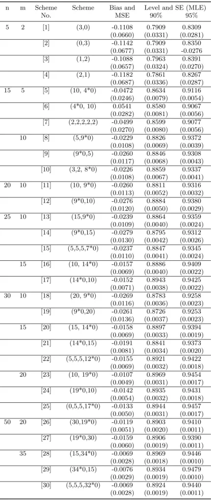
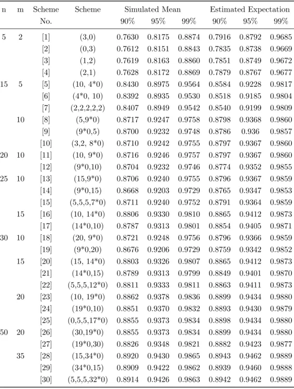
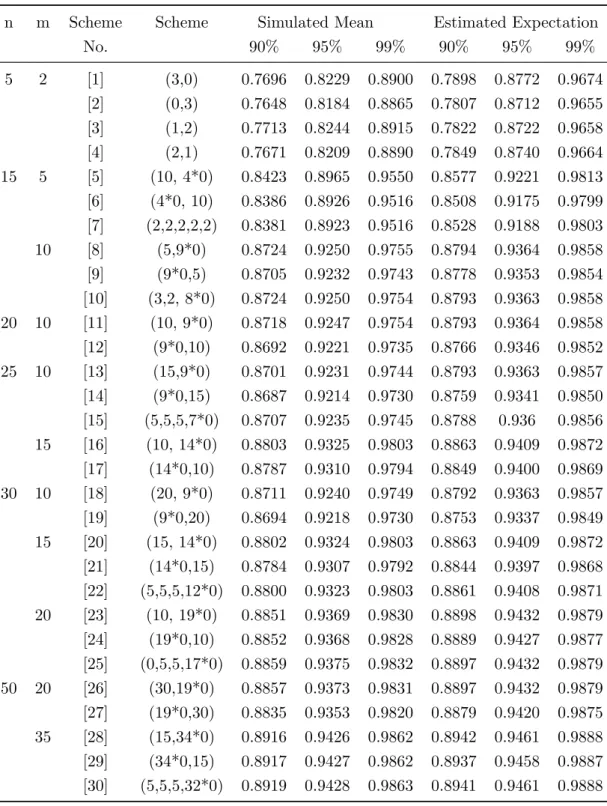
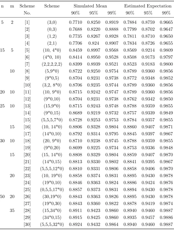
distribution of a k-unit series system with half-logistic distribution as the component life distribution In Table 1 scheme (a, b) stands for R1 = a and R2 = b. Similar meaning holds for schemes described through completely specified vector, while scheme (10,4∗0) meansR1 = 10 and rest fourRisare zero. i.e. R2 =R3 =R4 =R5 = 0. A simulation was carried out for 2-unit, 3-unit and 5-unit series system (i.e. k=2, 3 and 5) with λ = 1. EM algorithm and Newton-Raphson method are used to compute MLE. For each particular progressive censoring scheme, 10,000 sets of observations were generated. The bias, MSE, confidence levels with their standard errors (SE) for the corresponding confidence intervals for λ are displayed in Table 1 - 3 for k=2, 3 and 5 respectively. The bias, MSE, confidence levels with their SE for the confidence intervals for reliability function are displayed in Table 4 - 6 for k=2, 3 and 5 respectively. The simulated mean coverage and the estimated expectation of the tolerance interval are given in Table 7 -9. (+MSE and SE are given in parenthesis.)
Table 1: Bias, MSE+, Confidence levels and its SE+ for MLE (k=2) n m Scheme Scheme Bias and Level and SE-MLE Level and SE-log(MLE)
No. MSE 90% 95% 90% 95% 5 2 [1] (3,0) -0.0708 0.7481 0.7802 0.8411 0.8883 (0.3379) (0.0377) (0.0343) (0.0267) (0.0198) [2] (0,3) -0.0654 0.7525 0.7824 0.8445 0.8934 (0.3529) (0.0372) (0.0341) (0.0263) (0.0190) [3] (1,2) -0.0694 0.7540 0.7884 0.8489 0.8907 (0.3497) (0.0371) (0.0334) (0.0257) (0.0195) [4] (2,1) -0.0642 0.7520 0.7868 0.8427 0.8900 (0.3559) (0.0373) (0.0335) (0.0265) (0.0196) 15 5 [5] (10, 4*0) -0.0248 0.8339 0.8656 0.8727 0.9263 (0.1425) (0.0092) (0.0078) (0.0074) (0.0046) [6] (4*0, 10) -0.0196 0.8325 0.8693 0.8807 0.9313 (0.1624) (0.0093) (0.0076) (0.0070) (0.0043) [7] (2,2,2,2,2) -0.0205 0.8315 0.8643 0.8777 0.9303 (0.1546) (0.0093) (0.0078) (0.0072) (0.0043) 10 [8] (5,9*0) -0.0121 0.8652 0.9041 0.8902 0.9401 (0.0702) (0.0078) (0.0058) (0.0065) (0.0038) [9] (9*0,5) -0.0141 0.8680 0.9037 0.8941 0.9434 (0.0723) (0.0076) (0.0058) (0.0063) (0.0036) [10] (3,2, 8*0) -0.0134 0.8694 0.9057 0.8894 0.9368 (0.0713) (0.0076) (0.0057) (0.0066) (0.0039) 20 10 [11] (10, 9*0) -0.0117 0.8669 0.9045 0.8863 0.9391 (0.0705) (0.0058) (0.0043) (0.005) (0.0029) [12] (9*0,10) -0.0086 0.8686 0.9069 0.8936 0.9423 (0.0767) (0.0057) (0.0042) (0.0048) (0.0027) 25 10 [13] (15,9*0) -0.0167 0.8679 0.9070 0.8927 0.9398 (0.0693) (0.0046) (0.0034) (0.0038) (0.0023) [14] (9*0,15) -0.0161 0.8613 0.8973 0.8829 0.9356 (0.0805) (0.0048) (0.0037) (0.0041) (0.0024) [15] (5,5,5,7*0) -0.0106 0.8641 0.9033 0.8893 0.9401 (0.0733) (0.0047) (0.0035) (0.0039) (0.0023) 15 [16] (10, 14*0) -0.0099 0.8792 0.9198 0.8952 0.9455 (0.0464) (0.0042) (0.003) (0.0038) (0.0021) [17] (14*0,10) -0.0123 0.8745 0.9160 0.8935 0.9458 (0.0499) (0.0044) (0.0031) (0.0038) (0.0021) 30 10 [18] (20, 9*0) -0.0079 0.8676 0.9070 0.8889 0.9366 (0.0725) (0.00380 (0.0028) (0.0033) (0.002) [19] (9*0,20) -0.0100 0.8637 0.8994 0.8888 0.9389 (0.0844) (0.0039) (0.003) (0.0033) (0.0019) 15 [20] (15, 14*0) -0.0089 0.8745 0.9142 0.8865 0.9400 (0.0481) (0.0037) (0.0026) (0.0034) (0.0019) [21] (14*0,15) -0.0087 0.8792 0.9171 0.8940 0.9460 (0.0523) (0.0035) (0.0025) (0.0032) (0.0017) [22] (5,5,5,12*0) -0.0073 0.8777 0.9219 0.8960 0.9437 (0.0474) (0.0036) (0.0024) (0.0031) (0.0018) 20 [23] (10, 19*0) -0.0040 0.8859 0.9281 0.8942 0.9452 (0.0355) (0.0034) (0.0022) (0.0032) (0.0017) [24] (19*0,10) -0.0064 0.8891 0.9287 0.8973 0.9460 (0.0366) (0.0033) (0.0022) (0.0031) (0.0017) [25] (0,5,5,17*0) -0.0064 0.8839 0.9273 0.8946 0.9449 (0.0356) (0.0034) (0.0022) (0.0031) (0.0017) 50 20 [26] (30,19*0) -0.0058 0.8827 0.9245 0.8945 0.9440 (0.0360) (0.0021) (0.0014) (0.0019) (0.0011) [27] (19*0,30) -0.0095 0.8773 0.9218 0.8892 0.9423 (0.0411) (0.0022) (0.0014) (0.002) (0.0011) 35 [28] (15,34*0) -0.0021 0.8920 0.9350 0.8950 0.9467 (0.0207) (0.0019) (0.0012) (0.0019) (0.0010) [29] (34*0,15) -0.0054 0.8920 0.9346 0.8980 0.9473 (0.0211) (0.0019) (0.0012) (0.0018) (0.0010) [30] (5,5,5,32*0) -0.0044 0.8898 0.9342 0.8962 0.9444 (0.0205) (0.0020) (0.0012) (0.0019) (0.0011)
Table 2: Bias, MSE+, Confidence levels and its SE+ for MLE (k=3) n m Scheme Scheme Bias and Level and SE-MLE Level and SE-log(MLE)
No. MSE 90% 95% 90% 95% 5 2 [1] (3,0) -0.0492 0.7498 0.7796 0.8368 0.8927 (0.3704) (0.0375) (0.0344) 0.0273 (0.0192) [2] (0,3) -0.0535 0.7506 0.7858 0.8496 0.8980 (0.3822) (0.0374) (0.0337) (0.0256) (0.0183) [3] (1,2) -0.0356 0.7606 0.7934 0.8535 0.9016 (0.3921) (0.0364 (0.0328) (0.0250) (0.0177) [4] (2,1) -0.0535 0.7549 0.7849 0.8443 0.8912 (0.3774) (0.0370) (0.0338 (0.0263) (0.0194) 15 5 [5] (10, 4*0) -0.0265 0.8251 0.8630 0.8742 0.9228 (0.1503) (0.0096) (0.0079) (0.0073) (0.0047) [6] (4*0, 10) -0.0210 0.8300 0.8662 0.8787 0.9272 (0.1705) (0.0094) (0.0077) (0.0071) (0.0045) [7] (2,2,2,2,2) -0.0271 0.8284 0.8612 0.8767 0.9246 (0.1635) (0.0095) (0.0080) (0.0072) (0.0046) 10 [8] (5,9*0) -0.0107 0.8658 0.9070 0.8922 0.9408 (0.0733) (0.0077) (0.0056) (0.0064) (0.0037) [9] (9*0,5) -0.0103 0.8657 0.9024 0.8868 0.9396 (0.0794) (0.0078 (0.0059) (0.0067) (0.0038) [10] (3,2, 8*0) -0.0117 0.8685 0.9042 0.8905 0.9390 (0.0719) (0.0076) (0.0058) (0.0065) (0.0038) 20 10 [11] (10, 9*0) -0.0136 0.8676 0.9055 0.8905 0.9426 (0.0720) (0.0057) (0.0043) (0.0049) (0.0027) [12] (9*0,10) -0.0120 0.8653 0.9043 0.8924 0.9421 (0.0818) (0.0058) (0.0043) (0.0048) (0.0027) 25 10 [13] (15,9*0) -0.0151 0.8612 0.8983 0.8815 0.9325 (0.0756) (0.0048) (0.0037) (0.0042) (0.0025) [14] (9*0,15) -0.0098 0.8644 0.9023 0.8889 0.9385 (0.0859) (0.0047) (0.0035) (0.0040) (0.0023) [15] (5,5,5,7*0) -0.0126 0.8639 0.9013 0.8875 0.9359 (0.0764) (0.0047) (0.0036) (0.0040) (0.0024) 15 [16] (10, 14*0) -0.0100 0.8714 0.9141 0.8881 0.9384 (0.0493) (0.0045) (0.0031) (0.0040) (0.0023) [17] (14*0,10) -0.0098 0.8755 0.9121 0.8903 0.9407 (0.0545) (0.0044) (0.0032) (0.0039) (0.0022) 30 10 [18] (20, 9*0) -0.0139 0.8649 0.9041 0.8878 0.9385 (0.0737) (0.0039) (0.0029) (0.0033) (0.0019) [19] (9*0, 20) -0.0045 0.8666 0.9014 0.8877 0.9377 (0.0894) (0.0039) (0.0030) (0.0033) (0.0019) 15 [20] (15, 14*0) -0.0104 0.8766 0.9156 0.8893 0.9419 (0.0493) (0.0036) (0.0026) (0.0033) (0.0018) [21] (14*0,15) -0.0091 0.8715 0.9137 0.8876 0.9379 (0.0563) (0.0037) (0.0026) (0.0033) (0.0019) [22] (5,5,5,12*0) -0.0110 0.8767 0.9158 0.8889 0.9419 (0.0497) (0.0036) (0.0026) (0.0033) (0.0018) 20 [23] (10, 19*0) -0.0084 0.8789 0.9245 0.8937 0.9424 (0.0369) (0.0035) (0.0023) (0.0032) (0.0018) [24] (19*0,10) -0.0052 0.8813 0.9252 0.8942 0.9428 (0.0395) (0.0035) (0.0023) (0.0032) (0.0018) [25] (0,5,5,17*0) -0.0043 0.8831 0.9257 0.8937 0.9437 (0.0378) (0.0034) (0.0023) (0.0032) (0.0018) 50 20 [26] (30,19*0) -0.0052 0.8821 0.9243 0.8894 0.9426 (0.0375) (0.0021) (0.0014) (0.0020) (0.0011) [27] (19*0,30) -0.0060 0.8839 0.9248 0.8955 0.9459 (0.0438) (0.0021) (0.0014) (0.0019) (0.0010) 35 [28] (15,34*0) -0.0043 0.8865 0.9317 0.8919 0.9441 (0.0212) (0.0020) (0.0013) (0.0019) (0.0011) [29] (34*0,15) -0.0025 0.8944 0.9404 0.8998 0.9473 (0.0223) (0.0019) (0.0011) (0.0018) (0.0010) [30] (5,5,5,32*0) -0.0028 0.8896 0.9364 0.8965 0.9449 (0.0215) (0.0020) (0.0012) (0.0019) (0.0010)
Table 3: Bias, MSE+, Confidence levels and its SE+ for MLE (k=5) n m Scheme Scheme Bias and Level and SE (MLE) Level and SE
(log(MLE)) No. MSE 90% 95% 90% 95% 5 2 [1] (3,0) -0.05431 0.7545 0.7878 0.8445 0.8924 (0.3776) (0.0370) (0.0334) (0.0263) (0.0192) [2] (0,3) -0.0283 0.7489 0.7825 0.8444 0.8959 (0.4394) (0.0376) (0.0340) (0.0263) (0.0187) [3] (1,2) -0.0329 0.7626 0.7932 0.8498 0.9024 (0.4076) (0.0362) (0.0328) (0.0255) (0.0176) [4] (2,1) -0.0372 0.7536 0.7861 0.8441 0.8948 (0.4153) (0.0371) (0.0336) (0.0263) (0.0188) 15 5 [5] (10, 4*0) -0.0191 0.8306 0.8668 0.8755 0.9279 (0.1563) (0.0094) (0.0077) (0.0073) (0.0045) [6] (4*0, 10) -0.0097 0.8273 0.8608 0.8750 0.9271 (0.1875) (0.0095) (0.0080) (0.0073) (0.0045) [7] (2,2,2,2,2) -0.0211 0.8252 0.8570 0.8703 0.9209 (0.1758) (0.0096) (0.0082) (0.0075) (0.0049) 10 [8] (5,9*0) -0.0138 0.8668 0.9050 0.8928 0.9384 (0.0761) (0.0077) (0.0057) (0.0064) (0.0039) [9] (9*0,5) -0.0107 0.8629 0.8959 0.8868 0.9375 (0.0842) (0.0079) (0.0062) (0.0067) (0.0039) [10] (3,2, 8*0) -0.0143 0.8562 0.8966 0.8827 0.9324 (0.0801) (0.0082) (0.0062) (0.0069) (0.0042) 20 10 [11] (10, 9*0) -0.0128 0.8641 0.9033 0.8893 0.9378 (0.0783) (0.0059) (0.0044) (0.0049) (0.0029) [12] (9*0,10) -0.0093 0.8680 0.9027 0.8897 0.9413 (0.0870) (0.0057) (0.0044) (0.0049) (0.0028) 25 10 [13] (15,9*0) -0.0134 0.8651 0.9032 0.8893 0.9365 (0.0777) (0.0047) (0.0035) (0.0039) (0.0024) [14] (9*0,15) -0.0133 0.8682 0.9025 0.8927 0.9419 (0.0870) (0.0046) (0.0035) (0.0038) (0.0022) [15] (5,5,5,7*0) -0.0079 0.8670 0.9058 0.8930 0.9400 (0.0797) (0.0046) (0.0034) (0.0038) (0.0023) 15 [16] (10, 14*0) -0.0110 0.8777 0.9171 0.8914 0.9409 (0.0515) (0.0043) (0.0030) (0.0039) (0.0022) [17] (14*0,10) -0.0093 0.8750 0.9158 0.8923 0.9426 (0.0580) (0.0044) (0.0031) (0.0038) (0.0022) 30 10 [18] (20, 9*0) -0.0138 0.8602 0.8968 0.8843 0.9362 (0.0791) (0.0040) (0.0031) (0.0034) (0.0020) [19] (9*0,20) -0.0064 0.8660 0.9018 0.8886 0.9375 (0.0920) (0.0039) (0.0030) (0.0033) (0.0020) 15 [20] (15, 14*0) -0.0097 0.8782 0.9188 0.8932 0.9419 (0.0517) (0.0036) (0.0025) (0.0032) (0.0018) [21] (14*0,15) -0.0022 0.8819 0.9234 0.8991 0.9468 (0.0578) (0.0035) (0.0024) (0.0030) (0.0017) [22] (5,5,5,12*0) -0.0095 0.8808 0.9204 0.8950 0.9427 (0.0517) (0.0035) (0.0024) (0.0031) (0.0018) 20 [23] (10, 19*0) -0.0066 0.8864 0.9239 0.8936 0.9458 (0.0389) (0.0034) (0.0023) (0.0032) (0.0017) [24] (19*0,10) -0.0071 0.8796 0.9226 0.8955 0.9445 (0.0424) (0.0035) (0.0024) (0.0031) (0.0017) [25] (0,5,5,17*0) -0.0067 0.8841 0.9262 0.8961 0.9423 (0.0391) (0.0034) (0.0023) (0.0031) (0.0018) 50 20 [26] (30,19*0) -0.0117 0.8801 0.9221 0.8947 0.9436 (0.0389) (0.0021) (0.0014) (0.0019) 0.0011 [27] (19*0,30) -0.0057 0.8840 0.9238 0.8939 0.9455 (0.0447) (0.0021) (0.0014) (0.0019) (0.0010) 35 [28] (15,34*0) -0.0059 0.8806 0.9316 0.8891 0.9434 (0.0228) (0.0021) (0.0013) (0.0020) (0.0011) [29] (34*0,15) -0.0030 0.8936 0.9378 0.8979 0.9468 (0.0242) (0.0019) (0.0012) (0.0018) (0.0010) [30] (5,5,5,32*0) -0.0022 0.8887 0.9416 0.9035 0.9511 (0.0219) (0.0020) (0.0011) (0.0017) (0.0009)
Table 4: Bias, MSE+, Confidence levels and its SE+ for R(t) (k=2) n m Scheme Scheme Bias and Level and SE (MLE)
No. MSE 90% 95% 5 2 [1] (3,0) -0.1108 0.7909 0.8309 (0.0660) (0.0331) (0.0281) [2] (0,3) -0.1142 0.7909 0.8350 (0.0677) (0.0331) -0.0276 [3] (1,2) -0.1088 0.7963 0.8391 (0.0657) (0.0324) (0.0270) [4] (2,1) -0.1182 0.7861 0.8267 (0.0687) (0.0336) (0.0287) 15 5 [5] (10, 4*0) -0.0472 0.8634 0.9116 (0.0246) (0.0079) (0.0054) [6] (4*0, 10) 0.0541 0.8580 0.9067 (0.0282) (0.0081) (0.0056) [7] (2,2,2,2,2) -0.0499 0.8599 0.9077 (0.0270) (0.0080) (0.0056) 10 [8] (5,9*0) -0.0229 0.8826 0.9372 (0.0108) (0.0069) (0.0039) [9] (9*0,5) -0.0260 0.8846 0.9308 (0.0117) (0.0068) (0.0043) [10] (3,2, 8*0) -0.0226 0.8859 0.9337 (0.0108) (0.0067) (0.0041) 20 10 [11] (10, 9*0) -0.0260 0.8811 0.9316 (0.0113) (0.0052) (0.0032) [12] (9*0,10) -0.0276 0.8884 0.9380 (0.0120) (0.0050) (0.0029) 25 10 [13] (15,9*0) -0.0239 0.8864 0.9359 (0.0109) (0.0040) (0.0024) [14] (9*0,15) -0.0279 0.8795 0.9312 (0.0130) (0.0042) (0.0026) [15] (5,5,5,7*0) -0.0237 0.8847 0.9345 (0.0110) (0.0041) (0.0024) 15 [16] (10, 14*0) -0.0157 0.8886 0.9409 (0.0069) (0.0040) (0.0022) [17] (14*0,10) -0.0152 0.8943 0.9425 (0.0071) (0.0038) (0.0022) 30 10 [18] (20, 9*0) -0.0269 0.8783 0.9258 (0.0116) (0.0036) (0.0023) [19] (9*0,20) -0.0261 0.8726 0.9253 (0.0136) (0.0037) (0.0023) 15 [20] (15, 14*0) -0.0158 0.8897 0.9394 (0.0069) (0.0033) (0.0019) [21] (14*0,15) -0.0191 0.8841 0.9373 (0.0081) (0.0034) (0.0020) [22] (5,5,5,12*0) -0.0155 0.8921 0.9422 (0.0069) (0.0032) (0.0018) 20 [23] (10, 19*0) -0.0107 0.8969 0.9454 (0.0049) (0.0031) (0.0017) [24] (19*0,10) -0.0142 0.8935 0.9431 (0.0054) (0.0032) (0.0018) [25] (0,5,5,17*0) -0.0133 0.8944 0.9457 (0.0050) (0.0031) (0.0017) 50 20 [26] (30,19*0) -0.0119 0.8903 0.9410 (0.0051) (0.0020) (0.0011) [27] (19*0,30) -0.0159 0.8906 0.9390 (0.0060) (0.0019) (0.0011) 35 [28] (15,34*0) -0.0069 0.8969 0.9446 (0.0028) (0.0018) (0.0010) [29] (34*0,15) -0.0076 0.8934 0.9479 (0.0029) (0.0019) (0.0010) [30] (5,5,5,32*0) -0.0069 0.8924 0.9440 (0.0028) (0.0019) (0.0011)
Table 5: Bias, MSE+, Confidence levels and its SE+ for R(t) (k=3) n m Scheme Scheme Bias and Level and SE (MLE)
No. MSE 90% 95% 5 2 [1] (3,0) -0.0947 0.7412 0.7829 (0.0570) (0.0384) (0.0340) [2] (0,3) -0.0880 0.7470 0.7823 (0.0578) (0.0378) (0.0341) [3] (1,2) -0.0886 0.7510 0.7878 (0.0570) (0.0374) (0.0334) [4] (2,1) -0.0896 0.7463 0.7854 (0.0570) (0.0379) (0.0337) 15 5 [5] (10, 4*0) -0.0435 0.8423 0.8914 (0.0254) (0.0089) (0.0065) [6] (4*0, 10) -0.0455 0.8302 0.8784 (0.0287) (0.0094) (0.0071) [7] (2,2,2,2,2) -0.0456 0.8334 0.8828 (0.0275) (0.0093) (0.0069) 10 [8] (5,9*0) -0.0247 0.8723 0.9193 (0.0128) (0.0074) (0.0049) [9] (9*0,5) -0.0247 0.8706 0.9166 (0.0136) (0.0075) (0.0051) [10] (3,2, 8*0) -0.0228 0.8657 0.9189 (0.0129) (0.0078) (0.0050) 20 10 [11] (10, 9*0) -0.0229 0.8650 0.9164 (0.0129) (0.0058) (0.0038) [12] (9*0,10) -0.0244 0.8691 0.9199 (0.0140) (0.0057) (0.0037) 25 10 [13] (15,9*0) -0.0234 0.8638 0.9140 (0.0130) (0.0047) (0.0031) [14] (9*0,15) -0.0244 0.8675 0.9146 (0.0146) (0.0046) (0.0031) [15] (5,5,5,7*0) -0.0228 0.8703 0.9161 (0.0131) (0.0045 (0.0031) 15 [16] (10, 14*0) -0.0149 0.8772 0.9282 (0.0085) (0.0043) (0.0027) [17] (14*0,10) -0.0174 0.8764 0.9290 (0.0093) (0.0043) nn(0.0026) 30 10 [18] (20, 9*0) -0.0240 0.8693 0.9219 (0.0127) (0.0038) (0.0024) [19] (9*0,20) -0.0249 0.8606 0.9133 (0.0151) (0.0040) (0.0026) 15 [20] (15, 14*0) -0.015 0.8795 0.9286 (0.0085) (0.0035) (0.0022) [21] (14*0,15) -0.0157 0.8836 0.9325 (0.0092) (0.0034) (0.0021) [22] (5,5,5,12*0) -0.0166 0.8776 0.9279 (0.0087) (0.0036) (0.0022) 20 [23] (10, 19*0) -0.0115 0.8863 0.9389 (0.0062) (0.0034) (0.0019) [24] (19*0,10) -0.0129 0.8887 0.9385 (0.0066) (0.0033) (0.0019) [25] (0,5,5,17*0) -0.0127 0.8783 0.9295 (0.0064) (0.0036) (0.0022) 50 20 [26] (30,19*0) -0.0106 0.8860 0.9359 (0.0064) (0.0020) (0.0012) [27] (19*0,30) -0.0127 0.8809 0.9323 (0.0074) (0.0021) (0.0013) 35 [28] (15,34*0) -0.0078 0.8872 0.9387 (0.0036) (0.0020) (0.0012) [29] (34*0,15) -0.0072 0.8872 0.9408 (0.0038) (0.0020) (0.0011) [30] (5,5,5,32*0) -0.0065 0.8909 0.9392 (0.0035) (0.0019) (0.0011)
Table 6: Bias, MSE+, Confidence levels and its SE+ for R(t) (k=5) n m Scheme Scheme Bias and Level and SE (MLE)
No. MSE 90% 95% 5 2 [1] (3,0) -0.0348 0.6993 0.7390 (0.0340) (0.0421) (0.0390 [2] (0,3) -0.0363 0.7000 0.7319 (0.0347) (0.0420) (0.0392) [3] (1,2) -0.0341 0.7020 0.7344 (0.0349) (0.0418) (0.0390) [4] (2,1) -0.0341 0.7028 0.7364 (0.0343) (0.0418) (0.0388) 15 5 [5] (10, 4*0) -0.0203 0.8093 0.8515 (0.0176) (0.0103) (0.0084) [6] (4*0, 10) -0.0165 0.8024 0.8437 (0.0197) (0.0106) (0.0088) [7] (2,2,2,2,2) -0.0193 0.7933 0.8396 (0.0198) (0.0109) (0.0090) 10 [8] (5,9*0) -0.0126 0.8493 0.8907 (0.0100) (0.0085) (0.0065) [9] (9*0,5) -0.0133 0.8360 0.8808 (0.0109) (0.0091) (0.0070) [10] (3,2, 8*0) -0.0117 0.8493 0.8956 (0.0101) (0.0085) (0.0062) 20 10 [11] (10, 9*0) -0.0124 0.8436 0.8871 (0.0104) (0.0066) (0.0050) [12] (9*0,10) -0.0107 0.8366 0.8852 (0.0115) (0.0068) (0.0051) 25 10 [13] (15,9*0) -0.0133 0.8450 0.8931 (0.0102) (0.0052) (0.0038) [14] (9*0,15) -0.0116 0.8465 0.8919 (0.0112) (0.0052) (0.0039) [15] (5,5,5,7*0) -0.0123 0.8414 0.8900 (0.0105) (0.0053) (0.0039) 15 [16] (10, 14*0) -0.0089 0.8705 0.9134 (0.0069) (0.0045) (0.0032) [17] (14*0,10) -0.0092 0.8586 0.9025 (0.0078) (0.0049) (0.0035) 30 10 [18] (20, 9*0) -0.0120 0.8492 0.8970 (0.0101) (0.0043) (0.0031) [19] (9*0,20) -0.0106 0.8432 0.8864 (0.0116) (0.0044) (0.0034) 15 [20] (15, 14*0) -0.0095 0.8617 0.9108 (0.0070) (0.0040) (0.0027) [21] (14*0,15) -0.0087 0.8570 0.9054 0.0079 (0.0041) (0.0029) [22] (5,5,5,12*0) -0.0069 0.8596 0.9079 (0.0072) (0.0040) (0.0028) 20 [23] (10, 19*0) -0.0063 0.8729 0.9186 (0.0054) (0.0037) (0.0025) [24] (19*0,10) -0.0069 0.8705 0.9182 (0.0058) (0.0038) (0.0025) [25] (0,5,5,17*0) -0.0065 0.8717 0.9168 (0.0055) (0.0037) (0.0025) 50 20 [26] (30,19*0) -0.0077 0.8712 0.9178 (0.0054) (0.0022) (0.0015) [27] (19*0,30) -0.0069 0.8663 0.9142 (0.0063) (0.0023) (0.0016) 35 [28] (15,34*0) -0.0045 0.8849 0.9355 (0.0031) (0.0020) (0.0012) [29] (34*0,15) -0.0046 0.8855 0.9315 (0.0033) (0.0020) (0.0013) [30] (5,5,5,32*0) -0.0035 0.8828 0.9311 (0.0034) (0.0020) (0.0013)
Table 7: Simulated mean and estimated expectation of the approximate β- expectation tolerance interval for k=2
n m Scheme Scheme Simulated Mean Estimated Expectation
No. 90% 95% 99% 90% 95% 99% 5 2 [1] (3,0) 0.7630 0.8175 0.8874 0.7916 0.8792 0.9685 [2] (0,3) 0.7612 0.8151 0.8843 0.7835 0.8738 0.9669 [3] (1,2) 0.7619 0.8163 0.8860 0.7851 0.8749 0.9672 [4] (2,1) 0.7628 0.8172 0.8869 0.7879 0.8767 0.9677 15 5 [5] (10, 4*0) 0.8430 0.8975 0.9564 0.8584 0.9228 0.9817 [6] (4*0, 10) 0.8392 0.8935 0.9530 0.8518 0.9185 0.9804 [7] (2,2,2,2,2) 0.8407 0.8949 0.9542 0.8540 0.9199 0.9809 10 [8] (5,9*0) 0.8717 0.9247 0.9758 0.8798 0.9368 0.9860 [9] (9*0,5) 0.8700 0.9232 0.9748 0.8786 0.936 0.9857 [10] (3,2, 8*0) 0.8710 0.9242 0.9755 0.8797 0.9367 0.9860 20 10 [11] (10, 9*0) 0.8716 0.9246 0.9757 0.8797 0.9367 0.9860 [12] (9*0,10) 0.8704 0.9232 0.9746 0.8774 0.9352 0.9855 25 10 [13] (15,9*0) 0.8706 0.9240 0.9755 0.8796 0.9367 0.9859 [14] (9*0,15) 0.8668 0.9203 0.9729 0.8765 0.9347 0.9853 [15] (5,5,5,7*0) 0.8711 0.9240 0.9752 0.8791 0.9364 0.9859 15 [16] (10, 14*0) 0.8806 0.9330 0.9810 0.8865 0.9412 0.9873 [17] (14*0,10) 0.8787 0.9313 0.9801 0.8854 0.9405 0.9871 30 10 [18] (20, 9*0) 0.8721 0.9248 0.9756 0.8796 0.9366 0.9859 [19] (9*0,20) 0.8676 0.9206 0.9729 0.8759 0.9342 0.9852 15 [20] (15, 14*0) 0.8803 0.9326 0.9807 0.8865 0.9412 0.9873 [21] (14*0,15) 0.8789 0.9313 0.9799 0.8849 0.9401 0.9870 [22] (5,5,5,12*0) 0.8811 0.9333 0.9811 0.8863 0.9411 0.9873 20 [23] (10, 19*0) 0.8862 0.9378 0.9836 0.8899 0.9434 0.9880 [24] (19*0,10) 0.8851 0.9370 0.9832 0.8893 0.9430 0.9879 [25] (0,5,5,17*0) 0.8855 0.9373 0.9834 0.8898 0.9434 0.9880 50 20 [26] (30,19*0) 0.8855 0.9373 0.9834 0.8899 0.9434 0.9880 [27] (19*0,30) 0.8826 0.9348 0.9821 0.8882 0.9423 0.9877 35 [28] (15,34*0) 0.8920 0.9430 0.9865 0.8943 0.9462 0.9889 [29] (34*0,15) 0.8909 0.9422 0.9862 0.8939 0.9460 0.9888 [30] (5,5,5,32*0) 0.8914 0.9426 0.9863 0.8942 0.9462 0.9889
Table 8: Simulated mean and estimated expectation of the approximate β- expectation tolerance interval for k=3
n m Scheme Scheme Simulated Mean Estimated Expectation
No. 90% 95% 99% 90% 95% 99% 5 2 [1] (3,0) 0.7696 0.8229 0.8900 0.7898 0.8772 0.9674 [2] (0,3) 0.7648 0.8184 0.8865 0.7807 0.8712 0.9655 [3] (1,2) 0.7713 0.8244 0.8915 0.7822 0.8722 0.9658 [4] (2,1) 0.7671 0.8209 0.8890 0.7849 0.8740 0.9664 15 5 [5] (10, 4*0) 0.8423 0.8965 0.9550 0.8577 0.9221 0.9813 [6] (4*0, 10) 0.8386 0.8926 0.9516 0.8508 0.9175 0.9799 [7] (2,2,2,2,2) 0.8381 0.8923 0.9516 0.8528 0.9188 0.9803 10 [8] (5,9*0) 0.8724 0.9250 0.9755 0.8794 0.9364 0.9858 [9] (9*0,5) 0.8705 0.9232 0.9743 0.8778 0.9353 0.9854 [10] (3,2, 8*0) 0.8724 0.9250 0.9754 0.8793 0.9363 0.9858 20 10 [11] (10, 9*0) 0.8718 0.9247 0.9754 0.8793 0.9364 0.9858 [12] (9*0,10) 0.8692 0.9221 0.9735 0.8766 0.9346 0.9852 25 10 [13] (15,9*0) 0.8701 0.9231 0.9744 0.8793 0.9363 0.9857 [14] (9*0,15) 0.8687 0.9214 0.9730 0.8759 0.9341 0.9850 [15] (5,5,5,7*0) 0.8707 0.9235 0.9745 0.8788 0.936 0.9856 15 [16] (10, 14*0) 0.8803 0.9325 0.9803 0.8863 0.9409 0.9872 [17] (14*0,10) 0.8787 0.9310 0.9794 0.8849 0.9400 0.9869 30 10 [18] (20, 9*0) 0.8711 0.9240 0.9749 0.8792 0.9363 0.9857 [19] (9*0,20) 0.8694 0.9218 0.9730 0.8753 0.9337 0.9849 15 [20] (15, 14*0) 0.8802 0.9324 0.9803 0.8863 0.9409 0.9872 [21] (14*0,15) 0.8784 0.9307 0.9792 0.8844 0.9397 0.9868 [22] (5,5,5,12*0) 0.8800 0.9323 0.9803 0.8861 0.9408 0.9871 20 [23] (10, 19*0) 0.8851 0.9369 0.9830 0.8898 0.9432 0.9879 [24] (19*0,10) 0.8852 0.9368 0.9828 0.8889 0.9427 0.9877 [25] (0,5,5,17*0) 0.8859 0.9375 0.9832 0.8897 0.9432 0.9879 50 20 [26] (30,19*0) 0.8857 0.9373 0.9831 0.8897 0.9432 0.9879 [27] (19*0,30) 0.8835 0.9353 0.9820 0.8879 0.9420 0.9875 35 [28] (15,34*0) 0.8916 0.9426 0.9862 0.8942 0.9461 0.9888 [29] (34*0,15) 0.8917 0.9427 0.9862 0.8937 0.9458 0.9887 [30] (5,5,5,32*0) 0.8919 0.9428 0.9863 0.8941 0.9461 0.9888
Table 9: Simulated mean and estimated expectation of the approximate β- expectation tolerance interval for k=5
n m Scheme Scheme Simulated Mean Estimated Expectation
No. 90% 95% 99% 90% 95% 99% 5 2 [1] (3,0) 0.7710 0.8250 0.8919 0.7884 0.8759 0.9665 [2] (0,3) 0.7688 0.8220 0.8888 0.7799 0.8702 0.9647 [3] (1,2) 0.7735 0.8267 0.8928 0.7811 0.8710 0.9650 [4] (2,1) 0.7706 0.824 0.8907 0.7834 0.8726 0.9655 15 5 [5] (10, 4*0) 0.8459 0.8997 0.9568 0.8569 0.9214 0.9809 [6] (4*0, 10) 0.8414 0.8950 0.9528 0.8508 0.9173 0.9797 [7] (2,2,2,2,2) 0.8399 0.8939 0.9521 0.8523 0.9183 0.9800 10 [8] (5,9*0) 0.8722 0.9250 0.9754 0.8789 0.9360 0.9856 [9] (9*0,5) 0.8704 0.9231 0.9738 0.8772 0.9348 0.9852 [10] (3,2, 8*0) 0.8706 0.9235 0.9744 0.8789 0.9360 0.9856 20 10 [11] (10, 9*0) 0.8715 0.9242 0.9747 0.8789 0.9360 0.9856 [12] (9*0,10) 0.8704 0.9231 0.9738 0.8762 0.9342 0.9850 25 10 [13] (15,9*0) 0.8715 0.9243 0.9748 0.8788 0.9359 0.9855 [14] (9*0,15) 0.8689 0.9219 0.9732 0.8757 0.9339 0.9849 [15] (5,5,5,7*0) 0.8728 0.9253 0.9753 0.8784 0.9357 0.9855 15 [16] (10, 14*0) 0.8806 0.9328 0.9804 0.8860 0.9407 0.9871 [17] (14*0,10) 0.8792 0.9314 0.9795 0.8845 0.9397 0.9867 30 10 [18] (20, 9*0) 0.8710 0.9238 0.9745 0.8788 0.9359 0.9855 [19] (9*0,20) 0.8699 0.9225 0.9734 0.8753 0.9336 0.9848 15 [20] (15, 14*0) 0.8808 0.9329 0.9804 0.8859 0.9407 0.9870 [21] (14*0,15) 0.8813 0.9330 0.9802 0.8841 0.9395 0.9867 [22] (5,5,5,12*0) 0.8810 0.9331 0.9806 0.8858 0.9406 0.9870 20 [23] (10, 19*0) 0.8858 0.9374 0.9831 0.8895 0.9430 0.9878 [24] (19*0,10) 0.8846 0.9363 0.9824 0.8886 0.9424 0.9876 [25] (0,5,5,17*0) 0.8857 0.9373 0.9831 0.8894 0.9430 0.9878 50 20 [26] (30,19*0) 0.8843 0.9363 0.9826 0.8895 0.9430 0.9878 [27] (19*0,30) 0.8843 0.9360 0.9822 0.8878 0.9419 0.9874 35 [28] (15,34*0) 0.8911 0.9423 0.9860 0.8940 0.9460 0.9887 [29] (34*0,15) 0.8915 0.9425 0.9860 0.8935 0.9457 0.9886 [30] (5,5,5,32*0) 0.8924 0.9432 0.9864 0.8940 0.9460 0.9887
6 Real Data Application
Consider following real data which represents failure times, for a specific type of electrical insulation that was subjected to a continuously increasing voltage stress given by Lawless (2011).
12.3, 21.8, 24.4, 28.6, 43.2, 46.9, 70.7, 75.3, 95.5, 98.1, 138.6, 151.9.
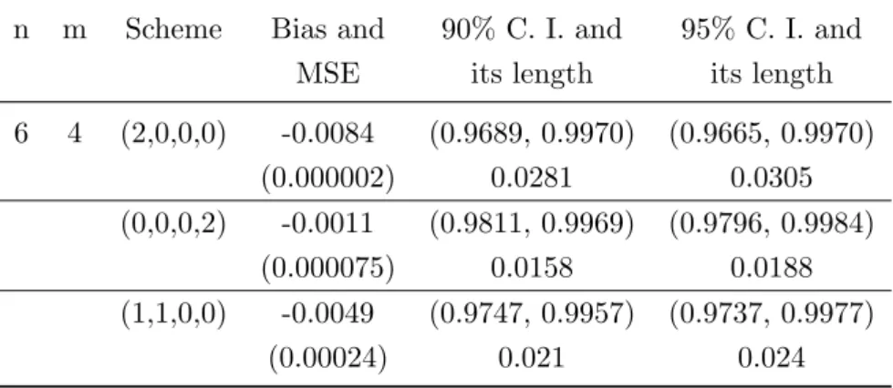
According to Balakrishnan and Chan (1992), half-logistic distribution satisfactory fit to this data. We consider this data as outcome for lifetime for two unit series system. We use this data with three censoring schemes as (2,0,0,0), (0,0,0,2) and (1,1,0,0). We obtain reliability estimate for time period t=1. MLE of reliability estimate and its MSE is given in Table 10. We construct confidence interval based on MLE. These 90% and 95% confidence intervals and their lengths are presented in same Table.
Table 10: Bias, MSE+, Confidence intervals and its length for R(t)
n m Scheme Bias and 90% C. I. and 95% C. I. and
MSE its length its length
6 4 (2,0,0,0) -0.0084 (0.9689, 0.9970) (0.9665, 0.9970) (0.000002) 0.0281 0.0305 (0,0,0,2) -0.0011 (0.9811, 0.9969) (0.9796, 0.9984) (0.000075) 0.0158 0.0188 (1,1,0,0) -0.0049 (0.9747, 0.9957) (0.9737, 0.9977) (0.00024) 0.021 0.024
Method of MLE using EM algorithm and confidence interval based on MLE of relia-bility function gives best performance for real data. Bias is small in case of conventional censoring scheme whereas MSE is small in case of progressive censoring scheme. Length of confidence interval is small in case of conventional censoring scheme.
7 Conclusion and Discussion
Simulation study results indicate that, the bias, MSE of the MLE and reliability estimate decrease with increase in sample size n and increase in the effective sample size m. Same trend is observed in case of SE of confidence level of confidence intervals. The MSE is relatively smaller for progressive Type-II censoring scheme as compared with conventional Type-II censoring scheme. Confidence levels of confidence interval using log-transformed MLE are better than the confidence levels of confidence interval using MLE. SE for confidence levels of confidence intervals using log-transformed MLE is
smaller than SE for confidence levels of confidence intervals using MLE. Confidence levels of confidence intervals of reliability function are better for large sample size.
β-expectation tolerance interval shows good results. As sample size n and effective sample size m increases the estimated expectation and simulated mean approaches to nominal coverage. Estimated expectation and simulated mean have better coverage for progressive Type-II censoring scheme than conventional Type-II censoring scheme, for small sample size. As number of units in system (k) increases the simulated mean decreases, but estimated expectation increases.
EM algorithm method works well for small sample size and for smaller effective sam-ple size. Overall both conventional Type-II censoring scheme and progressive Type-II censoring scheme give better results. The MSE of progressive Type-II censoring method is smaller than the MSE of conventional censoring method, while bias, confidence in-terval and β-expectation tolerance interval perform equally good for both the methods. The results reported in this paper can also be applied when k is replaced by any known positive real number.
Aknowledgment
The authors are grateful to the editor and the learned referee for making constructive and valuable comments which have significantly improved the contents of this article.
References
Asgharzadeh, A. and Valiollahi, R. (2011). Estimation of the scale parameter of the lomax distribution under progressive censoring. International Journal of Statistics & Economics, 6(S11):37–48.
Atwood, C. L. (1984). Approximate tolerance intervals, based on maximum likelihood estimates. Journal of the American Statistical Association, 79(386):459–465.
Balakrishnan, N. (2007). Progressive censoring methodology: an appraisal. Test, 16(2):211–259.
Balakrishnan, N. and Aggarwala, R. (2000). Progressive censoring: theory, methods, and applications. Springer.
Balakrishnan, N. and Asgharzadeh, A. (2005). Inference for the scaled half-logistic dis-tribution based on progressively type-ii censored samples. Communications in Statis-ticsTheory and Methods, 34(1):73–87.
Balakrishnan, N. and Chan, P. (1992). Estimation for the scaled half logistic distribution under type ii censoring. Computational statistics & data analysis, 13(2):123–141. Balakrishnan, N., Kannan, N., Lin, C., and Wu, S. (2004). Inference for the extreme
value distribution under progressive type-ii censoring. Journal of Statistical Compu-tation and Simulation, 74(1):25–45.
estimation for gaussian distribution, based on progressively type-ii censored samples.
Reliability, IEEE Transactions on, 52(1):90–95.
Balakrishnan, N. and Sandhu, R. (1995). A simple simulational algorithm for generating progressive type-ii censored samples. The American Statistician, 49(2):229–230. Cohen, A. C. (1963). Progressively censored samples in life testing. Technometrics,
5(3):327–339.
Dempster, A. P., Laird, N. M., and Rubin, D. B. (1977). Maximum likelihood from incomplete data via the em algorithm. Journal of the Royal Statistical Society. Series B (Methodological), pages 1–38.
Iliopoulos, G. and Balakrishnan, N. (2011). Exact likelihood inference for laplace distri-bution based on type-ii censored samples. Journal of Statistical Planning and Infer-ence, 141(3):1224–1239.
Kim, C. and Han, K. (2010). Estimation of the scale parameter of the half-logistic distribution under progressively type ii censored sample. Statistical Papers, 51(2):375– 387.
Krishna, H. and Kumar, K. (2011). Reliability estimation in lindley distribution with progressively type ii right censored sample. Mathematics and Computers in Simula-tion, 82(2):281–294.
Krishna, H. and Kumar, K. (2013). Reliability estimation in generalized inverted expo-nential distribution with progressively type ii censored sample. Journal of Statistical Computation and Simulation, 83(6):1007–1019.
Krishna, H. and Malik, M. (2012). Reliability estimation in maxwell distribution with progressively type-ii censored data.Journal of Statistical Computation and Simulation, 82(4):623–641.
Kumbhar, R. and Shirke, D. (2004). Tolerance limits for lifetime distribution of k-unit parallel system. Journal of Statistical Computation and Simulation, 74(3):201–213. Lawless, J. F. (2011).Statistical models and methods for lifetime data, volume 362. John
Wiley & Sons.
Little, R. J. and Rubin, D. B. (2002). Statistical analysis with missing data.
Louis, T. A. (1982). Finding the observed information matrix when using the em al-gorithm. Journal of the Royal Statistical Society. Series B (Methodological), pages 226–233.
Mann, N. R. (1969). Exact three-order-statistic confidence bounds on reliable life for a weibull model with progressive censoring. Journal of the American Statistical Associ-ation, 64(325):306–315.
Mann, N. R. (1971). Best linear invariant estimation for weibull parameters under progressive censoring. Technometrics, 13(3):521–533.
McLachlan, G. and Krishnan, T. (2007).The EM algorithm and extensions, volume 382. John Wiley & Sons.
Meeker, W. Q. and Escobar, L. A. (1998). Statistical methods for reliability data, volume 314. John Wiley & Sons.
Ng, H. (2005). Parameter estimation for a modified weibull distribution, for progressively type-ii censored samples. Reliability, IEEE Transactions on, 54(3):374–380.
Ng, H., Chan, P., and Balakrishnan, N. (2002). Estimation of parameters from progres-sively censored data using em algorithm. Computational Statistics & Data Analysis, 39(4):371–386.
Potdar, K. and Shirke, D. (2012). Inference for the distribution of a k-unit parallel system with exponential distribution as the component life distribution based on type-ii progressively censored sample. Int. J. Agricult. Stat. Sci, 8(2):503–517.
Potdar, K. and Shirke, D. (2013a). Inference for the parameters of generalized inverted family of distributions. InProdStat Forum, volume 6, pages 18–28.
Potdar, K. and Shirke, D. (2013b). Reliability estimation for the distribution of a k-unit parallel system with rayleigh distribution as the component life distribution. In International Journal of Engineering Research and Technology, volume 2. ESRSA Publications.
Potdar, K. and Shirke, D. (2014). Inference for the scale parameter of lifetime distri-bution of k-unit parallel system based on progressively censored data. Journal of Statistical Computation and Simulation, 84(1):171–185.
Pradhan, B. (2007). Point and interval estimation for the lifetime distribution of a k-unit parallel system based on progressively type-ii censored data. Economic Quality Control, 22(2):175–186.
Pradhan, B. and Kundu, D. (2009). On progressively censored generalized exponential distribution. Test, 18(3):497–515.