Working Paper M11/02
Methodology
Non-Parametric Bootstrap Mean
Squared Error Estimation For
M-Quantile Estimators Of Small Area
Averages, Quantiles And Poverty
Indicators
Stefano Marchetti, Nikos Tzavidis, Monica Pratesi Abstract
Small area estimation is conventionally concerned with the estimation of small area averages and totals. More recently emphasis has been also placed on the estimation of poverty indicators and of key quantiles of the small area distribution function using robust models for example, the M-quantile small area model (Chambers and Tzavidis, 2006). In parallel to point estimation, Mean Squared Error (MSE) estimation is an equally crucial and challenging task. However, while analytic MSE estimation for small area averages is possible, analytic MSE estimation for quantiles and poverty indicators is extremely difficult. Moreover, one of the main criticisms of the analytic MSE estimator for M-quantile estimates of small area averages proposed by Chambers and Tzavidis (2006) and Chambers et al. (2009) is that it can be unstable when the area-specific sample sizes are small.
Non-parametric Bootstrap Mean Squared Error
Estimation for M-quantile Estimators of Small Area
Averages, Quantiles and Poverty Indicators
Stefano Marchetti∗
Department of Statistics and Mathematics Applied to Economics, University of Pisa, Via Ridolfi, 10 - 56124 Pisa (PI), Italy
Nikos Tzavidis∗
Social Statistics and Southampton Statistical Sciences Research Institute, University of Southampton, Highfield, SO17 1BJ, Southampton, UK
Monica Pratesi∗
Department of Statistics and Mathematics Applied to Economics, University of Pisa, Via Ridolfi, 10 - 56124 Pisa (PI), Italy
Abstract
Small area estimation is conventionally concerned with the estimation of small area averages and totals. More recently emphasis has been also placed on the estimation of poverty indicators and of key quantiles of the small area distribution function using robust models for example, the M-quantile small area model (Chambers and Tzavidis, 2006). In parallel to point estimation, Mean Squared Error (MSE) estimation is an equally crucial and challenging task. However, while analytic MSE estimation for small area averages is possible, analytic MSE estimation for quantiles and poverty indicators is extremely difficult. Moreover, one of the main criticisms of the analytic MSE estimator for M-quantile estimates of small area averages proposed by Chambers and Tzavidis (2006) and Chambers et al. (2009) is that it can be unstable when the area-specific sample sizes are small.
∗Corresponding author
Email addresses: [email protected](Stefano Marchetti),
We propose a non-parametric bootstrap framework for MSE estimation for small area averages, quantiles and poverty indicators estimated with the M-quantile small area model. Because the small area statistics we consider in this paper can be expressed as functionals of the Chambers-Dunstan esti-mator of the population distribution function, the proposed non-parametric bootstrap presents an extension of the work by Lombardia et al. (2003). Alternative bootstrap schemes, based on resampling empirical or smoothed residuals, are studied and the asymptotic properties are discussed in the light of the work by Lombardia et al. (2003). Emphasis is also placed on second or-der properties of MSE estimators with results suggesting that the bootstrap MSE estimator is more stable than corresponding analytic MSE estimators. The proposed bootstrap is evaluated in a series of simulation studies under different parametric assumptions for the model error terms and different sce-narios for the area-specific sample and population sizes. We finally present results from the application of the proposed MSE estimator to real income data from the European Survey of Income and Living Conditions (EU-SILC) in Italy and provide information on the availability of R functions that can be used for implementing the proposed estimation procedures in practice.
Keywords: Chambers-Dunstan estimator, Income distribution, Domain estimation, Poverty mapping, Resampling methods, Robust estimation
1. Introduction
Sample surveys provide an effective way of obtaining estimates for pop-ulation characteristics. Estimation, however, can become difficult when the focus is on domains (areas) with small sample sizes. The term ‘small areas’ is typically used to describe domains whose sample sizes are not large enough to allow sufficiently precise direct estimation, i.e. estimation based only on the sample data from the domain (Rao, 2003). When direct estimation is not possible, one has to rely upon alternative model-based methods for produc-ing small area estimates. Small area estimation is conventionally concerned with the estimation of small area averages and totals. More recently empha-sis has been also placed on the estimation of poverty indicators and of key quantiles of the small area distribution function (Molina et al., 2010) using the M-quantile small area model (Chambers and Tzavidis, 2006).
Estimating the precision of small area estimates is both an important and challenging task. Despite the fact that MSE estimation for M-quantile small
area averages has been studied fairly extensively (Chambers and Tzavidis, 2006; Chambers et al., 2009), MSE estimation for more complex small area statistics e.g. for poverty indicators estimated with the M-quantile model is unexplored. What is more, analytic MSE estimation for complex statistics is difficult. For example, all small area statistics we consider in this pa-per can be expressed as functionals of the population distribution function, which can be consistently estimated by using the Chambers-Dunstan estima-tor (Chambers and Dunstan, 1986). Although the asymptotic behaviour of this estimator was studied by Chambers and Dunstan (1986) and asymptotic expressions for the bias and the variance were derived by Chambers et al. (1992), the use of these expressions has proven to be impractical. This mo-tivates the work in this paper in which we propose a unified non-parametric bootstrap framework for MSE estimation for small area averages, quantiles and poverty indicators - in particular, for the Head Count Ratio (HCR) and for the Poverty Gap (PG)- estimated with the M-quantile small area model. The proposed bootstrap is based on resampling empirical or smoothed M-quantile model residuals and presents an extension of the work by Lombardia et al. (2003) to small area estimation with the M-quantile model. The choice of a non-parametric bootstrap scheme, instead of a parametric one, is dic-tated by the fact that the M-quantile small area model does not make explicit parametric assumptions about the model error terms. This is in contrast to the conventional unit level area random effects model which assumes that the unit level and area level error terms are Gaussian. MSE estimation us-ing parametric, instead of non-parametric, bootstrap has been recently used by Sinha and Rao (2009) for estimating the MSE of the Robust Empirical Best Linear Unbiased Predictor (REBLUP) of the small area average and by Molina and Rao (2010) for estimating the MSE of small area poverty indi-cators estimated by using the Empirical Best Prediction (EBP) approach.
The complexity of the small area target parameters we consider in this paper is only one way of motivating the use of bootstrap. There is one addi-tional reason as to why one may consider using a bootstrap MSE estimator. As we mentioned above, analytic MSE estimation for M-quantile estimates of small area averages has been already proposed. Although this estimator is bias robust against mispecifications of the model assumptions, one of its main criticisms is that it can be unstable when used with small area-specific sample sizes. Second order properties of MSE estimators are, however, also very important. For this reason, a further aim of this paper is to also study the stability of the non-parametric bootstrap MSE estimator and compare
this to the stability of corresponding analytic MSE estimators.
The paper is organised as follows. In Section 2 we review the M-quantile small area model and present point estimation for small area averages, poverty indicators and quantiles. Analytic MSE estimation for estimates of small area averages is reviewed. Although the emphasis here is on MSE estimation, rather than on point estimation, we must stress that estimation of poverty indicators under the M-quantile model is presented for the first time in this paper. However, comparisons with alternative poverty estimation approaches -e.g. the EBP method of Molina and Rao (2010)- will be discussed elsewhere. In Section 3 we present the non-parametric bootstrap scheme and provide a sketch of its asymptotic properties. In Section 4 the performance of the proposed MSE estimator is empirically evaluated under different paramet-ric assumptions for the model error terms and for the small area sample and population sizes. For the case of small area averages the bootstrap MSE esti-mator is also compared to the analytic MSE estiesti-mator proposed by Chambers and Tzavidis (2006) and Tzavidis et al. (2010). Using real income data from the EU-SILC survey in Italy, in Section 5 we apply the bootstrap MSE es-timator for computing the accuracy of estimates of income averages, income quantiles and poverty indicators for Provinces in Tuscany. Access to software that implements the proposed estimation procedures is important for users of small area estimation methods and Section 6 provides information on the availability of R functions. Finally, in Section 7 we conclude the paper with some final remarks.
2. Small area estimation by using the M-quantile model
In what follows we assume that a vector of p auxiliary variable xij is
known for each population unit i in small areaj = 1, . . . , m and that values of the variable of interest y are available from a random sample, s, that includes units from all the small areas of interest. We denote the population size, sample size, sampled part of the population and non sampled part of the population in area j respectively by Nj, nj, sj and rj. We assume that
the sum over the areas of Nj and nj is equal to N and n respectively. We
further assume that conditional on covariate information for example, design variables, the sampling design is ignorable.
A recently proposed approach to small area estimation is based on the use of a quantile/M-quantile regression model (Chambers and Tzavidis, 2006). The classical regression model summarises the behaviour of the mean of a
random variable y at each point in a set of covariates x. Instead, quantile regression summarises the behaviour of different parts (e.g. quantiles) of the conditioned distribution of y at each point in the set of thex’s. In the linear case, quantile regression leads to a family of hyper-planes indexed by a real number q ∈ (0,1). For a given value of q, the corresponding model shows how the qth quantile of the conditional distribution of y varies with x. For example, for q = 0.1 the quantile regression hyperplane separates the lower 10% of the conditional distribution from the remaining 90%.
Let us for the moment and for notational simplicity drop subscript j. Suppose that (xT
i , yi), i= 1,· · · , ndenotes the observed values for a random
sample consisting of n units, where xT
i are row p-vectors of a known design
matrix X and yi is a scalar response variable corresponding to a realisation
of a continuous random variable with unknown continuous cumulative distri-bution functionF. A linear regression model for theqth conditional quantile of yi given xi is
Qyi(q|xi) =xi
Tβ(q).
An estimate of the qth regression parameter β(q) is obtained by minimizing
n X i=1 n |yi−xTi β(q)| (1−q)I(yi−xTiβ(q)≤0) +qI(yi−xTi β(q)>0) o .
Quantile regression presents a generalization of median regression and expectile regression (Newey and Powell, 1987) a ‘quantile-like’ generaliza-tion of mean regression. M-quantile regression (Breckling and Chambers, 1988) integrates these concepts within a framework defined by a ‘quantile-like’ generalization of regression based on influence functions (M-regression). The M-quantile of order q for the conditional density of y given the set of covariates x,f(y|x), is defined as the solutionM Qy(q|x;ψ) of the estimating
equationR
ψq{y−M Qy(q|x;ψ)}f(y|x)dy= 0, whereψqdenotes an
asymmet-ric influence function, which is the derivative of an asymmetasymmet-ric loss function
ρq. A linear M-quantile regression modelyi givenxi is one where we assume
that
M Qy(q|xi;ψ) = xiTβψ(q), (1)
and estimates of βψ(q) are obtained by minimizing
n X i=1 ρq yi−xiTβψ(q) . (2)
Different regression models can be defined as special cases of (2). In partic-ular, by varying the specifications of the asymmetric loss function ρq we
ob-tain the expectile, M-quantile and quantile regression models as special cases. When ρq is the square loss function we obtain the linear expectile regression
model ifq 6= 0.5 (Newey and Powell, 1987) and the standard linear regression model ifq= 0.5. Whenρqis the loss function described by Koenker and
Bas-sett (1978) we obtain the linear quantile regression. Throughout this paper we will take the linear M-quantile regression model to be defined by whenρq
is the Huber loss function (Breckling and Chambers, 1988). Setting the first derivative of (2) equal to zero leads to the following estimating equations
n
X
i=1
ψq(riq)xi =0,
where riq =yi −xTi βψ(q),ψq(riq) = 2ψ(s−1riq){qI(riq >0) + (1−q)I(riq ≤
0)} and s > 0 is a suitable estimate of scale. For example, in the case
of robust regression, s = median|riq|/0.6745. Since the focus of our paper
is on M-type estimation, we use the Huber Proposal 2 influence function,
ψ(u) = uI(−c ≤ u ≤ c) +c·sgn(u). Provided that the tuning constant c
is strictly greater than zero, estimates of βψ(q) are obtained using iterative weighted least squares (IWLS).
2.1. Estimators of small area averages
Chambers and Tzavidis (2006) extended the use of M-quantile regression models to small area estimation. Following their development (see also Kokic et al., 1997; Aragon et al., 2005), these authors characterize the conditional variability across the population of interest by the M-quantile coefficients of the population units. For unit i with values yi and xi, this coefficient is
the value θi such that M Qy(θi|xi;ψ) = yi The M-quantile coefficients are
determined at the population level. Consequently, if a hierarchical structure does explain part of the variability in the population data, then we expect units within clusters (domains) defined by this hierarchy to have similar M-quantile coefficients. When the conditional M-quantiles are assumed to follow the linear model (1), with βψ(q) a sufficiently smooth function of q, Chambers and Tzavidis (2006) suggested a plug in (na¨ıve) estimator of the average value of y in areaj
ˆ mM Qj =Nj−1h X i∈sj yi+ X i∈rj xTi βˆψ(ˆθj) i , j = 1, . . . , m, (3)
where ˆθj is an estimate of the average value of the M-quantile coefficients
of the units in area j. The area-specific M-quantile coefficients, ˆθj, can be
viewed as pseudo-random effects. Empirical work indeed indicates that the area-specific M-quantile coefficients are positively and highly correlated with the estimated random area-specific effects obtained with the nested error re-gression small area model. Chambers and Tzavidis (2006) also observed that the na¨ıve M-quantile estimator (3) can be biased, especially in the presence of heteroskedastic and/or asymmetric errors. This observation motivated the work in Tzavidis et al. (2010). In particular, these authors proposed a bias adjusted M-quantile estimator for the small area average that is de-rived by using an estimator of the finite population distribution function such as the Chambers-Dunstan estimator (Chambers and Dunstan, 1986). The Chambers-Dunstan estimator of the small area distribution function is of the form ˆ FjCD(t) = Nj−1h X i∈sj I(yi ≤t) +n−j1 X k∈rj X i∈sj I(xTkβˆψ(ˆθj) +ei ≤t) i .
Estimates of θj and βψ(θj) are obtained following Chambers and Tzavidis
(2006) and ei = yi −xTi βˆψ(ˆθj) are model residuals. The M-quantile
bias-adjusted estimator of the average of y in small area j is then defined as ˆ mCDj = Z +∞ −∞ yd ˆFjCD(y) =Nj−1h X i∈sj yi+ X i∈rj ˆ yi+ (1−fj) X i∈sj ei i . (4)
where fj = njNj−1 is the sampling fraction in area j and ˆyi = xTi βˆψ(ˆθj), i ∈ rj. The bias correction in (4) means that this estimator has higher
variability than (3). Nevertheless, because of its bias robust properties, (4) is usually preferred, over the na¨ıve M-quantile estimator, in practice. Finally, as we will also see in the next section, by using the Chambers-Dunstan estimator one can define a general framework for small area estimation that extends beyond the estimation of small area averages.
Analytic MSE estimation for M-quantile estimators of small area averages is described in Chambers and Tzavidis (2006) and Chambers et al. (2009). In particular, Chambers et al. (2009) proposed an analytic mean squared error
estimator that is a first order approximation to the mean squared error of estimator (4). These authors noted that since an iteratively reweighted least squares algorithm is used to calculate the M-quantile regression fit at ˆθj,
ˆ
βψ(ˆθj) = (XTsWsjXs)
−1
XTsWsjys
where Xs and ys denote the matrix of sample x values and the vector of
sample y values respectively, and Wsj denotes the diagonal weight matrix
of order n that defines the estimator of the M-quantile regression coefficient with q = ˆθj. It immediately follows that (4) can be written
ˆ mCDj =wTsjys, (5) where wsj = (wij) = n −1 j ∆sj + (1−N −1 j nj)WjXs(XTsWjXs)−1(xrj −xsj)
with ∆sj denoting the n-vector that ‘picks out’ the sample units from area j. Herexsj and xrj denote the sample and non-sample means of xin area j.
Also, these weights are ‘locally calibrated’ on x since X
i∈s
wijxi = ¯xsj + (1−fj)(¯xrj −x¯sj) = ¯xj.
A first order approximation to the mean squared error of (5) then treats the weights as fixed and applies standard methods of robust mean squared error estimation for linear estimators of population quantities (Royall and Cumberland, 1978). With this approach, the prediction variance of ˆmCD
j is estimated by d V ar( ˆmCDj ) = m X g=1 X i∈sg λijg yi−xiβˆψ(ˆθg) 2 , (6)
where λijg = [(wij −1)2 + (nj − 1)−1(Nj − nj)]I(g = j) + wig2I(g 6= j).
Empirical studies show that the analytic MSE estimator (6) is bias robust against misspecification of the model (Chambers et al., 2009). However, its main criticism is that it can be unstable especially with small area-specific sample sizes.
2.2. Estimators of small area poverty indicators and quantiles
Although small area averages are widely used in small area applications, relying only on averages may not be very informative. This is the case for
example in economic applications where estimates of average income may not provide an accurate picture of the area wealth due to the high within area inequality. Our goal in this section is to also express quantiles and specific poverty indicators as functionals of the Chambers-Dunstan estimator of the population distribution function.
With regards to the estimation of small area quantiles, an estimate of quantileφfor small areaj is the value ˆq(j;φ) obtained by a numerical solution to the following estimating equation
Z qˆ(j;φ)
−∞
d ˆFjCD(t) =φ. (7)
Estimating poverty indicators at disaggregated geographical levels is also important. In this paper we focus on the estimation of the incidence of poverty orHead Count Ratio (HCR) and of thePoverty Gap (PG) as defined by Foster et al. (1984). Denoting by t the poverty line, different poverty indicators are defined by using
Fα,i =
t−yi
t
α
I(yi ≤t) i= 1, . . . N.
The population poverty indicators in small area j,Fα,j, can then be
decom-posed as follows, Fα,j =Nj−1 h X i∈sj Fα,i+ X i∈rj Fα,i i .
In particular, setting α = 0, F0,j defines the HCR while setting α = 1 F1,j defines the PG in small area j. Hence, one approach for estimating
the HCR in small area j is by using the Chambers-Dunstan estimator of the distribution function and the M-quantile model for predicting for out of sample units as follows,
ˆ F0,j = Nj−1 h X i∈sj I(yi ≤ t) + n−j1 X k∈rj X i∈sj I(xTkβˆψ(ˆθj) + ei ≤ t) i . (8)
Similarly, an estimator of the poverty gap for area j
ˆ F1,j =Nj−1 h X i∈sj t−yi t I(yi ≤t) +n−j1X k∈rj X i∈sj t−xT kβˆψ(ˆθj)−ei t I(xTkβˆψ(ˆθj) +ei ≤t) i . (9)
In practice the HCR and PG for area j can be estimated by using a Monte Carlo approach. The estimation procedure is as follows:
1 Fit the M-quantile small area model using the sample values ys and
obtain estimates ˆθj, ˆβψ(ˆθj), of θj and βψ(θj).
2 Draw an out of sample vector using
y∗k =xTkβˆψ(ˆθj) +e∗k, k ∈rj,
where e∗k, k ∈ rj is a vector of size Nj −nj drawn from the empirical
distribution function of the estimated M-quantile model residuals. 3 Repeat the processH times. Each time combine the sample data and
out of sample data for estimating F0,j and F1,j.
4 Average the results over H simulations.
The M-quantile approach for estimating poverty indicators is similar in spirit to the EBP approach proposed by Molina and Rao (2010). Note for example that yk∗, k ∈ rj is generated using xTkβˆψ(ˆθj) i.e. from the conditional
M-quantile model, where ˆθj plays the role of the area random effects in the
M-quantile modelling framework.
3. Non-parametric bootstrap MSE estimation
All small area target parameters we presented in Section 2 have been expressed as functionals of the Chambers-Dunstan estimator of the popula-tion distribupopula-tion funcpopula-tion. Unlike MSE estimapopula-tion for small area averages, analytic MSE estimation for small area poverty indicators and quantiles is complex. In this section we present a nonparametric bootstrap framework for MSE estimation of small area parameters estimated with the M-quantile model and the Chambers-Dunstan estimator.
Let us start with the M-quantile small area model
yij =xTijβψ(θj) +εij
where βψ(θj) is the unknown vector of M-quantile regression parameters
for the unknown area-specific M-quantile coefficient θj, and εij is the unit
parametric assumptions are being made. Using the sample data we obtain estimates ˆθj, ˆβψ(ˆθj), of θj and βψ(θj), and estimated model residuals eij = yij −xTijβˆψ(ˆθj). The target is to estimate the small area finite population
distribution function, or to be more precise a functional of this distribution function τ, by using the Chambers-Dunstan estimator and the M-quantile small area model,
ˆ FjCD(t) = Nj−1h X i∈sj I(yij ≤t) + X k∈rj ˆ G t−xTijβˆψ(ˆθj) i , (10)
where ˆG(u) is the empirical distribution, ˆG(u) = n−j1P
i∈sjI(eij ≤u), of the
model residuals eij. Using (10), we obtain estimates of the small area target
parameters we presented in Section 2, which we collectively denote by ˆτ. Given an estimator ˆGest(u) of the distribution of the residuals G(u) = P r(ε ≤ u), a bootstrap population, consistent with the M-quantile small area model, Ω∗ = {yij∗,xij}, can be generated by sampling from ˆGest(u) to
obtain ε∗ij,
yij∗ =xTijβˆψ(ˆθj) +ε∗ij, i= 1, . . . , Nj, j = 1, . . . , m.
For defining ˆGest(u) we consider two approaches: (1) sampling from the
empirical distribution function of the model residuals or (2) sampling from a smoothed distribution function of the model residuals. For each of the two above mentioned approaches, sampling can be done in two ways namely, by sampling from the distribution of all residuals without conditioning on the small area (unconditional approach) or by sampling from the distribution of the residuals within small area j (conditional approach). The empirical distribution of the residuals for the unconditional approach is
ˆ Gest(t) =n−1 m X j=1 X i∈sj I(eij −e¯s ≤t), (11)
where ¯es is the sample mean of the residuals eij, while for the conditional
approach the empirical distribution is ˆ Gjest(t) = n −1 j X i∈sj I(eij −e¯sj ≤t),
where ¯esj is the sample mean of the residuals in area j. The corresponding
and the conditional approaches are respectively ˆ Gest =n−1 m X j=1 X i∈sj K h−1(t−eij + ¯es) , (12) and ˆ Gjest(t) = n −1 j X i∈sj K h−j1(t−eij + ¯esj) ,
whereh >0 (orhj) is a smoothing parameter andK is the distribution
func-tion corresponding to a bounded symmetric kernel density k. Hence, there are four possible approaches for definingε∗ij. We suggest, however, using the unconditional, empirical or smoothed, approach. The reason is that in appli-cations of small area estimation sampling from the conditional distribution would rely on potentially a very small number of data points which can cause
ˆ
Gest(t) to be unstable. Let us now define the finite distribution function for
the bootstrap population as follows
Fj∗(t) = Nj−1h X
i∈sj
I(y∗ij ≤t) +X
i∈rj
I(y∗ij ≤t)i.
The bootstrap population distribution function can be estimated by selecting a without replacement sample from the bootstrap population and by using the Chambers-Dunstan estimator
ˆ Fj∗,CD(t) = Nj−1h X i∈sj I(yij∗ ≤t) +X k∈rj ˆ G∗ t−xT ijβˆ ∗ ψ( ˆθ∗j) i , (13)
where ˆβ∗ψ(ˆθj∗) are bootstrap sample estimates of the M-quantile model pa-rameters and ˆG∗ = n−1
j
P
i∈sjI(e
∗
ij ≤ u). Using (13) we obtain bootstrap
estimates, ˆτ∗, of the bootstrap population small area parameters τ∗.
The steps of the bootstrap procedure are as follows: starting from sam-ple s, selected from a finite population Ω without replacement, we fit the M-quantile small area model and obtain estimates of θj and βψ(θj) which
are used to compute the model residuals. We then generate B bootstrap populations, Ω∗b, using one of the previously described methods for
estimat-ing the distribution of the residuals, G(u). From each bootstrap population, Ω∗b, we select Lbootstrap samples using simple random sampling within the
bootstrap samples we obtain estimates ofτ. Bootstrap estimators of the bias and variance of the estimated target small area parameter, ˆτ, derived from the distribution function in area j are defined respectively by
d Bias(ˆτj) =B−1L−1 B X b=1 L X l=1 ˆ τj∗bl−τj∗b, d Var(ˆτj) = B−1L−1 B X b=1 L X l=1 ˆ τj∗bl−τ¯ˆj∗bl2 , where τ∗b
j is the small area parameter of the bth bootstrap population, ˆτ
∗bl j
is the small area parameter estimated by using (13) with the lth sample of the bth bootstrap population and ¯τˆj∗bl = L−1PL
l=1τˆ
∗bl
j . The bootstrap MSE
estimator of the estimated small area target parameter is then defined as
\
M SE(ˆτj) =Var(ˆd τj) +Bias(ˆd τj)2. (14)
3.1. A note on asymptotic properties
The asymptotic properties of the smoothed bootstrap method, under a linear model, have been studied by Lombardia et al. (2003). Here we com-ment on the validity of the assumptions by Lombardia et al. (2003) under the M-quantile model. To start with, we note that the superpopulation model assumed by Lombardia et al. (2003) is a special case of the linear M-quantile model when a squared loss function is used in (2) andq = 0.5 (see Breckling and Chambers, 1988; Newey and Powell, 1987). Under this model and using the assumptions on page 371 of their paper Lombardia et al. (2003) showed that the smoothed bootstrap estimator ˆF∗,CD(t) is consistent, in that its
be-haviour relative to the smoothed bootstrap population distribution function
F∗(t) is identical to the relationship between ˆFCD(t) and the
correspond-ing population distribution function F(t). The asymptotic behaviour of the latter was studied by Chambers et al. (1992) under assumptions relating to the superpopulation model density and the asymptotic behavior of the sampling fraction (H1-H3 on page 371 of Lombardia et al. (2003)). More-over, Lombardia et al. (2003) show that the smoothed bootstrap estimator is asymptotically normally distributed. The assumptions made by Lombar-dia et al. (2003) relate to the kernel function, the bandwidth parameter and the density g of G. In our case the assumptions about the kernel density
k and the bandwidth parameter h (K1 and K2 on page 371 of Lombardia et al. (2003)) hold and in our empirical evaluations we use the same kernel function and bandwidth selection method as those used by Lombardia et al. (2003). In addition, the assumptions about the superpopulation model and the asymptotic behavior of the sampling fraction (H1 to H4 on page 371) are reasonable assumptions also under the M-quantile linear model. Finally, conditional on the small areas the assumption of independence of the errors is also reasonable.
4. Empirical evaluations
In this section we use model-based Monte-Carlo simulations to empirically evaluate the performance of the bootstrap MSE estimator (14) when used to estimate the MSE of the M-quantile estimators of (a) the small area average (4), (b) the small area quantile (7), (c) the head count ratio (HCR) (8) and (d) the poverty gap (PG) (9). Moreover, since analytic MSE estimation for M-quantile estimates of small area averages is possible, the proposed boot-strap MSE estimator is also contrasted to the corresponding analytic MSE estimator (6) both in terms of bias and stability. The behaviour of the alter-native MSE estimators is assessed under two different parametric assump-tions for the model error terms namely, Normal and Chi-square errors, and two scenarios for the area-specific sample and population sizes. Finally, we also present results on how well estimators of small area averages, quantiles and poverty indicators estimate the corresponding population parameters.
In what follows subscript j identifies small areas, j = 1, . . . , m and sub-script i identifies units in a given area, i = 1, . . . , nj. Population data
Ω = (x, y) in m = 30 small areas are generated under two parametric sce-narios for the model error terms. Population data under the first parametric scenario were generated by using a unit level area random effects model with normally distributed random area effects and unit level errors as follows
yij = 3000−150∗xij +γj +εij,
where γj ∼ N(0,2002), εij ∼ N(0,8002), xij ∼ N(µj,1), µj ∼ U[4,10] and µj was held fixed over simulations. Similarly, under the second parametric
scenario population data were generated using
where now γj ∼ χ2(1), εij ∼ χ2(6) and xij was generated as in the first
scenario but with µj ∼U[8,11].
For each Monte Carlo simulation a within small areas random sample is selected from the corresponding generated population. Two scenarios for the population and sample sizes are investigated. Under the first scenario (denoted in the tables of results by λ = 0) the total population size is N = 8400 with small area-specific population sizes ranging between 150 ≤ Nj ≤
440. The total sample size is n = 840 and the area-specific sample sizes are ranging between 15 ≤ nj ≤ 44. Under the second scenario (denoted
in the tables of results by λ = 1) the total population size is N = 2820 with area-specific population sizes ranging between 50 ≤ Nj ≤150 and the
total sample size is n = 282 with area-specific sample sizes ranging between 5≤nj ≤15.
Using the sample data we obtain point estimates of small area averages with (4), of the 0.25, 0.50 and 0.75 percentiles of the distribution of y with (7) and of the HCR and PG with (8) and (9) respectively. For small area av-erages MSE estimation is performed using both the analytic MSE (6) and the bootstrap MSE estimator (14). For estimators of small area percentiles and poverty indicators MSE estimation is performed using the bootstrap MSE estimator (14). We run in totalH = 500 Monte-Carlo simulations. For boot-strap MSE estimation we used one bootboot-strap population (B = 1) from which we drew 400 bootstrap samples (L = 400). Because the evaluation of the bootstrap MSE estimator is taking place within a Monte-Carlo framework, the generation of a new Monte-Carlo population and of a new bootstrap population in each iteration is imitating the generation of many bootstrap populations. For the bootstrap MSE estimation we used the unconditional approach with both the empirical (11) and smoothed (12) versions of the error distribution. For the smoothed case, we use the Epanechnikov kernel density, k(u) = (3/4)(1−u2)I(|u|<1), where the smoothing parameterhin
(12) was chosen so that it minimizes the cross-validation criterion suggested by Bowman et al. (1998). That is, h was chosen in order to minimize
CV(h) =n−1 m X j=1 X i∈sj Z I(eij −¯es)≤t−G−i(t) 2 dt,
where G−i(t) is the version of G(t) that omits sample unit i (Li and Racine
(2007), section 1.5). To compute the smoothing parameter h in (12) we used the np package (Hayfield and Racine, 2008) in the R environment (R
Development Core Team, 2010).
Denoting by τj the true and unknown parameter and by ˆτj the
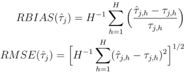
corre-sponding estimate, the performance of MSE estimators is evaluated using the relative bias and Root MSE (RMSE) defined by
RBIAS(ˆτj) =H−1 H X h=1 τˆj,h−τj,h τj,h RM SE(ˆτj) = h H−1 H X h=1 (ˆτj,h−τj,h)2 i1/2
Finally, coverage rates of 95% confidence intervals constructed by using the bootstrap MSE estimator are computed. Although the detailed results of coverage rates are not reported in the tables of results, we do provide sum-mary results of coverage rates in our commentary.
4.1. Results for small area averages
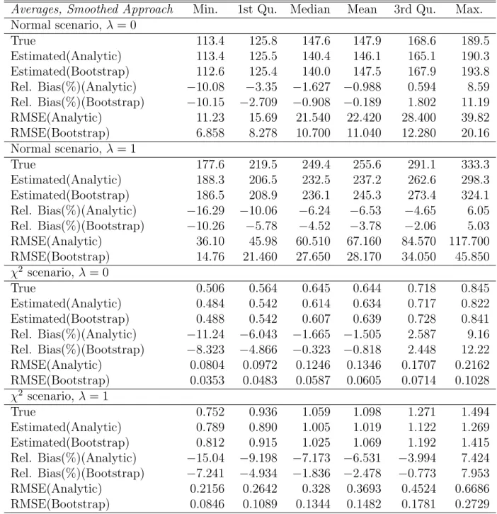
Table 1 presents the results for MSE estimation of M-quantile small area averages obtained with (4), under the two parametric scenarios and the two scenarios for the area-specific sample and population sizes, using the analytic MSE estimator (6) and the bootstrap MSE estimator (14). For bootstrap estimation we used the smoothed unconditional approach for estimating the distribution of the residuals. Results from the implementation of the em-pirical unconditional approach have been also produced but in the economy of space are not reported here. The table reports the distribution over ar-eas of the empirical, Monte Carlo RMSE, the estimated RMSE, the relative bias (%) of the estimated RMSE and the RMSE of the RMSE estimators, which is used for assessing the stability of the bootstrap and analytic MSE estimators.
These results suggest that for all scenarios we studied the analytic and the bootstrap MSE estimators track very well the empirical MSE and have on average reasonably low relative bias. However, the bootstrap MSE estimator appears to be notably more stable. In particular, the RMSE of the bootstrap MSE estimator is approximately half that of the analytic estimator (scenario with λ = 0) and differences become more pronounced for the smaller area sample sizes (scenario λ = 1). Therefore, there is evidence to suggest that the bootstrap MSE estimator is more stable than the analytic MSE estimator
Averages, Smoothed Approach Min. 1st Qu. Median Mean 3rd Qu. Max. Normal scenario, λ = 0 True 113.4 125.8 147.6 147.9 168.6 189.5 Estimated(Analytic) 113.4 125.5 140.4 146.1 165.1 190.3 Estimated(Bootstrap) 112.6 125.4 140.0 147.5 167.9 193.8 Rel. Bias(%)(Analytic) −10.08 −3.35 −1.627 −0.988 0.594 8.59 Rel. Bias(%)(Bootstrap) −10.15 −2.709 −0.908 −0.189 1.802 11.19 RMSE(Analytic) 11.23 15.69 21.540 22.420 28.400 39.82 RMSE(Bootstrap) 6.858 8.278 10.700 11.040 12.280 20.16 Normal scenario, λ = 1 True 177.6 219.5 249.4 255.6 291.1 333.3 Estimated(Analytic) 188.3 206.5 232.5 237.2 262.6 298.3 Estimated(Bootstrap) 186.5 208.9 236.1 245.3 273.4 324.1 Rel. Bias(%)(Analytic) −16.29 −10.06 −6.24 −6.53 −4.65 6.05 Rel. Bias(%)(Bootstrap) −10.26 −5.78 −4.52 −3.78 −2.06 5.03 RMSE(Analytic) 36.10 45.98 60.510 67.160 84.570 117.700 RMSE(Bootstrap) 14.76 21.460 27.650 28.170 34.050 45.850 χ2 scenario, λ = 0 True 0.506 0.564 0.645 0.644 0.718 0.845 Estimated(Analytic) 0.484 0.542 0.614 0.634 0.717 0.822 Estimated(Bootstrap) 0.488 0.542 0.607 0.639 0.728 0.841 Rel. Bias(%)(Analytic) −11.24 −6.043 −1.665 −1.505 2.587 9.16 Rel. Bias(%)(Bootstrap) −8.323 −4.866 −0.323 −0.818 2.448 12.22 RMSE(Analytic) 0.0804 0.0972 0.1246 0.1346 0.1707 0.2162 RMSE(Bootstrap) 0.0353 0.0483 0.0587 0.0605 0.0714 0.1028 χ2 scenario, λ = 1 True 0.752 0.936 1.059 1.098 1.271 1.494 Estimated(Analytic) 0.789 0.890 1.005 1.019 1.122 1.269 Estimated(Bootstrap) 0.812 0.915 1.025 1.069 1.192 1.415 Rel. Bias(%)(Analytic) −15.04 −9.198 −7.173 −6.531 −3.994 7.424 Rel. Bias(%)(Bootstrap) −7.241 −4.934 −1.836 −2.478 −0.773 7.953 RMSE(Analytic) 0.2156 0.2642 0.328 0.3693 0.4524 0.6686 RMSE(Bootstrap) 0.0846 0.1089 0.1344 0.1482 0.1781 0.2729
Table 1: Distribution over areas and simulations of the empirical, Monte Carlo RMSE, of the estimated RMSE (analytic and bootstrap), of the relative bias (%) of the RMSE estimators and of the RMSE of the RMSE estimators for M-quantile estimators of small area averages. Bootstrap results are produced using the unconditional smoothed approach.
proposed by Chambers and Tzavidis (2006) and hence it should be preferred in practical applications. The results using the empirical distribution, instead of the smoothed distribution of the residuals, are consistent with the results we present here. Figure 1 present averages, over simulations, of true and estimated, using (4), small area means. In the economy of space we present results only for the χ2 scenario and the Normal scenario with the smaller area sample sizes (λ = 1). These results show that estimates of small area averages are close to population values. The results for other scenarios are consistent with the ones we present here. Results for coverage rates of 95% confidence intervals for estimates of small area averages constructed by using the bootstrap MSE estimator are on average close to 95% for both parametric scenarios and for both scenarios of the area sample and population sizes.
4.2. Results for small area poverty indicators and percentiles
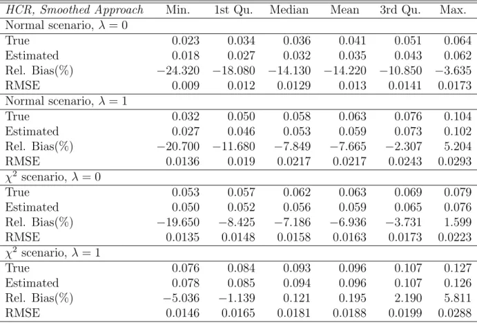
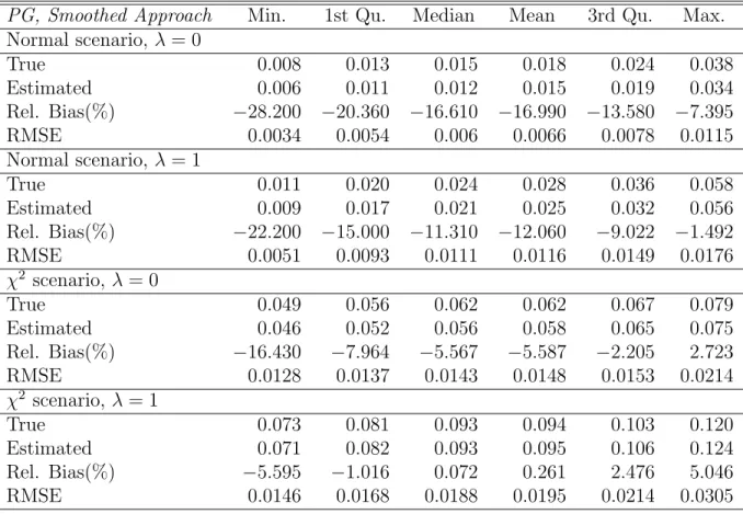
Tables 2 and 3 present results on the performance of the bootstrap MSE estimator (14) when used to estimate the MSE of estimates of HCR and PG obtained with (8) and (9) respectively. Bootstrap MSE estimation is implemented using the smoothed unconditional approach for estimating the distribution of the residuals. Results from the implementation of the empir-ical unconditional approach have been also produced but in the economy of space are not reported here. The tables report the distribution over areas of the empirical, Monte Carlo RMSE, the estimated RMSE, the relative bias of the bootstrap MSE and the RMSE of the RMSE estimator, which is used for assessing the stability of the bootstrap MSE estimator.
From tables 2 and 3 we see that the estimated RMSE for HCR and PG tracks well the entire distribution of the empirical RMSE, both for the Normal andχ2 scenarios. For the normal scenario, these results also show evidence of substantial relative bias ranging on average between (-16% , - 7.6%), which may be due to the large values of the error variance components we used for generating the Monte-Carlo population creating some instability when estimating an indicator. For the chi-square scenario the relative bias is sub-stantially lower ranging on average between (-6.9% , -0.19%). In any case the results on the relative bias must be interpreted with care since the values of the MSEs are small and hence even small differences will result in sub-stantial relative bias. This is the case even with values that agree up to the second decimal place. As expected, the variability of the RMSE estimator is greater when the sample size is smaller, however, given the decrease in the area sample sizes (see scenario λ = 1) the stability of the MSE estimator
HCR, Smoothed Approach Min. 1st Qu. Median Mean 3rd Qu. Max. Normal scenario, λ = 0 True 0.023 0.034 0.036 0.041 0.051 0.064 Estimated 0.018 0.027 0.032 0.035 0.043 0.062 Rel. Bias(%) −24.320 −18.080 −14.130 −14.220 −10.850 −3.635 RMSE 0.009 0.012 0.0129 0.013 0.0141 0.0173 Normal scenario, λ = 1 True 0.032 0.050 0.058 0.063 0.076 0.104 Estimated 0.027 0.046 0.053 0.059 0.073 0.102 Rel. Bias(%) −20.700 −11.680 −7.849 −7.665 −2.307 5.204 RMSE 0.0136 0.019 0.0217 0.0217 0.0243 0.0293 χ2 scenario, λ = 0 True 0.053 0.057 0.062 0.063 0.069 0.079 Estimated 0.050 0.052 0.056 0.059 0.065 0.076 Rel. Bias(%) −19.650 −8.425 −7.186 −6.936 −3.731 1.599 RMSE 0.0135 0.0148 0.0158 0.0163 0.0173 0.0223 χ2 scenario, λ = 1 True 0.076 0.084 0.093 0.096 0.107 0.127 Estimated 0.078 0.085 0.094 0.096 0.107 0.126 Rel. Bias(%) −5.036 −1.139 0.121 0.195 2.190 5.811 RMSE 0.0146 0.0165 0.0181 0.0188 0.0199 0.0288
Table 2: Distribution over areas and simulations of the empirical, Monte Carlo RMSE, of the bootstrap RMSE and of the relative Bias (%) and RMSE of the bootstrap RMSE estimator for the HCR. Results are produced using the unconditional smoothed approach.
PG, Smoothed Approach Min. 1st Qu. Median Mean 3rd Qu. Max. Normal scenario, λ = 0 True 0.008 0.013 0.015 0.018 0.024 0.038 Estimated 0.006 0.011 0.012 0.015 0.019 0.034 Rel. Bias(%) −28.200 −20.360 −16.610 −16.990 −13.580 −7.395 RMSE 0.0034 0.0054 0.006 0.0066 0.0078 0.0115 Normal scenario, λ = 1 True 0.011 0.020 0.024 0.028 0.036 0.058 Estimated 0.009 0.017 0.021 0.025 0.032 0.056 Rel. Bias(%) −22.200 −15.000 −11.310 −12.060 −9.022 −1.492 RMSE 0.0051 0.0093 0.0111 0.0116 0.0149 0.0176 χ2 scenario, λ = 0 True 0.049 0.056 0.062 0.062 0.067 0.079 Estimated 0.046 0.052 0.056 0.058 0.065 0.075 Rel. Bias(%) −16.430 −7.964 −5.567 −5.587 −2.205 2.723 RMSE 0.0128 0.0137 0.0143 0.0148 0.0153 0.0214 χ2 scenario, λ = 1 True 0.073 0.081 0.093 0.094 0.103 0.120 Estimated 0.071 0.082 0.093 0.095 0.106 0.124 Rel. Bias(%) −5.595 −1.016 0.072 0.261 2.476 5.046 RMSE 0.0146 0.0168 0.0188 0.0195 0.0214 0.0305
Table 3: Distribution over areas and simulations of the empirical, Monte Carlo RMSE, of the bootstrap RMSE and of the relative Bias (%) and RMSE of the bootstrap RMSE estimator for the PG. Results are produced using the unconditional smoothed approach.
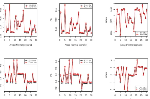
remains satisfactory. These stability results will be only effectively evaluated when compared to alternative MSE estimators of the HCR and PG. Cur-rently, the only alternative available is the parametric bootstrap proposed by Molina and Rao (2010). Figure 1 present averages, over simulations, of true and estimated, using (8) and (9), small area HCRs and PGs. In the economy of space we present results only for the χ2 scenario and the Normal senario with the smaller area sample sizes (λ = 1). These results show that estimates of small area HCRs and PGs are close to population values. The results for other scenarios are consistent with the ones we present here.
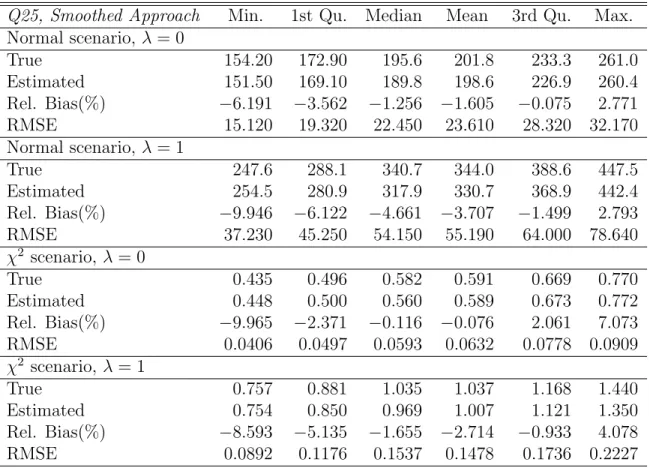
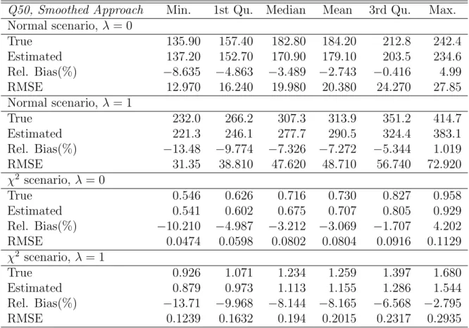
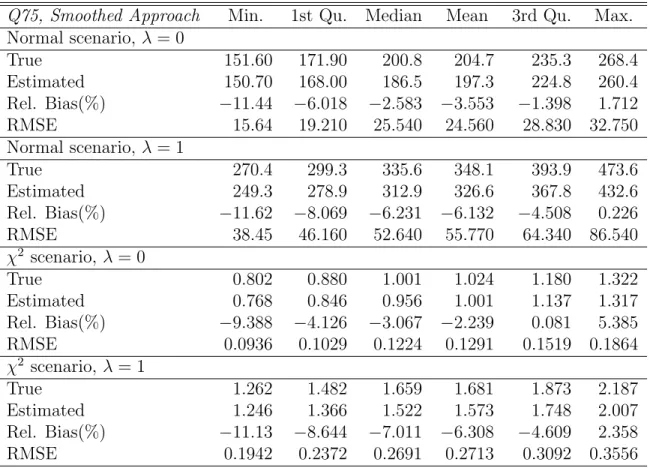
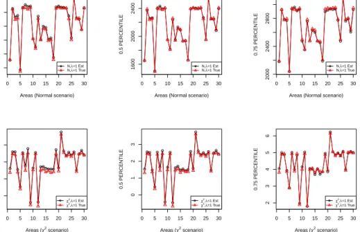
In tables 4, 5 and 6 we present MSE estimation results for the percentiles of y and more specifically for q = 0.25,0.5,0.75 estimated with (7). The ta-bles report the distribution over areas of the empirical, Monte Carlo RMSE, the estimated RMSE, the relative bias of the bootstrap RMSE and the RMSE of the RMSE estimators, which is used for assessing the stability of the bootstrap MSE estimator. Bootstrap MSE estimation is implemented using the smoothed unconditional approach for estimating the distribution of the residuals. Results from the implementation of the empirical unconditional approach have been also produced but in the economy of space are not re-ported here. The bootstrap MSE estimator tracks well the distribution of the empirical MSE of the three percentiles under both parametric scenarios and both scenarios for the small area sample sizes. Some underestimation is present but in terms of percentage relative bias this underestimation is not excessive. Figure 2 presents averages, over simulations, of true and es-timated, using (7), small area percentile estimates of q = 0.25,0.5,0.75. In the economy of space we present results only for theχ2 and Normal scenario
with the smaller area sample sizes (λ= 1). These results show that estimates of small area percentiles are close to population values. The results for other scenarios are consistent with the ones we present here.
Coverage rates of 95% confidence intervals for estimates of small area quantiles constructed by using the bootstrap MSE estimator range on aver-age between 93% to 95% for both parametric scenarios and for both scenarios of the area sample and population sizes. The coverage rates of 95% confi-dence intervals for estimates of small area poverty indicators (HCR and PG) constructed by using the bootstrap MSE estimator range on average between 90% to 94% for both parametric scenarios and for both scenarios of the area sample and population sizes.
The results we presented in the section indicate that the bootstrap MSE can be reliably used for estimating the MSE of M-quantile small area
av-Q25, Smoothed Approach Min. 1st Qu. Median Mean 3rd Qu. Max. Normal scenario, λ = 0 True 154.20 172.90 195.6 201.8 233.3 261.0 Estimated 151.50 169.10 189.8 198.6 226.9 260.4 Rel. Bias(%) −6.191 −3.562 −1.256 −1.605 −0.075 2.771 RMSE 15.120 19.320 22.450 23.610 28.320 32.170 Normal scenario, λ = 1 True 247.6 288.1 340.7 344.0 388.6 447.5 Estimated 254.5 280.9 317.9 330.7 368.9 442.4 Rel. Bias(%) −9.946 −6.122 −4.661 −3.707 −1.499 2.793 RMSE 37.230 45.250 54.150 55.190 64.000 78.640 χ2 scenario, λ = 0 True 0.435 0.496 0.582 0.591 0.669 0.770 Estimated 0.448 0.500 0.560 0.589 0.673 0.772 Rel. Bias(%) −9.965 −2.371 −0.116 −0.076 2.061 7.073 RMSE 0.0406 0.0497 0.0593 0.0632 0.0778 0.0909 χ2 scenario, λ = 1 True 0.757 0.881 1.035 1.037 1.168 1.440 Estimated 0.754 0.850 0.969 1.007 1.121 1.350 Rel. Bias(%) −8.593 −5.135 −1.655 −2.714 −0.933 4.078 RMSE 0.0892 0.1176 0.1537 0.1478 0.1736 0.2227
Table 4: Distribution over areas and simulations of the empirical, Monte Carlo RMSE, of the bootstrap RMSE and of the relative Bias (%) and the RMSE of the bootstrap RMSE estimator for the 0.25 percentile. Results are produced using the unconditional smoothed approach.
Q50, Smoothed Approach Min. 1st Qu. Median Mean 3rd Qu. Max. Normal scenario, λ = 0 True 135.90 157.40 182.80 184.20 212.8 242.4 Estimated 137.20 152.70 170.90 179.10 203.5 234.6 Rel. Bias(%) −8.635 −4.863 −3.489 −2.743 −0.416 4.99 RMSE 12.970 16.240 19.980 20.380 24.270 27.85 Normal scenario, λ = 1 True 232.0 266.2 307.3 313.9 351.2 414.7 Estimated 221.3 246.1 277.7 290.5 324.4 383.1 Rel. Bias(%) −13.48 −9.774 −7.326 −7.272 −5.344 1.019 RMSE 31.35 38.810 47.620 48.710 56.740 72.920 χ2 scenario, λ = 0 True 0.546 0.626 0.716 0.730 0.827 0.958 Estimated 0.541 0.602 0.675 0.707 0.805 0.929 Rel. Bias(%) −10.210 −4.987 −3.212 −3.069 −1.707 4.202 RMSE 0.0474 0.0598 0.0802 0.0804 0.0916 0.1129 χ2 scenario, λ = 1 True 0.926 1.071 1.234 1.259 1.397 1.680 Estimated 0.879 0.973 1.113 1.155 1.286 1.544 Rel. Bias(%) −13.71 −9.968 −8.144 −8.165 −6.568 −2.795 RMSE 0.1239 0.1632 0.194 0.2015 0.2317 0.2935
Table 5: Distribution over areas and simulations of the empirical, Monte Carlo RMSE, of the bootstrap RMSE and of the relative Bias (%) and the RMSE of the bootstrap RMSE estimator for the 0.5 percentile. Results are produced using the unconditional smoothed approach.
Q75, Smoothed Approach Min. 1st Qu. Median Mean 3rd Qu. Max. Normal scenario, λ = 0 True 151.60 171.90 200.8 204.7 235.3 268.4 Estimated 150.70 168.00 186.5 197.3 224.8 260.4 Rel. Bias(%) −11.44 −6.018 −2.583 −3.553 −1.398 1.712 RMSE 15.64 19.210 25.540 24.560 28.830 32.750 Normal scenario, λ = 1 True 270.4 299.3 335.6 348.1 393.9 473.6 Estimated 249.3 278.9 312.9 326.6 367.8 432.6 Rel. Bias(%) −11.62 −8.069 −6.231 −6.132 −4.508 0.226 RMSE 38.45 46.160 52.640 55.770 64.340 86.540 χ2 scenario, λ = 0 True 0.802 0.880 1.001 1.024 1.180 1.322 Estimated 0.768 0.846 0.956 1.001 1.137 1.317 Rel. Bias(%) −9.388 −4.126 −3.067 −2.239 0.081 5.385 RMSE 0.0936 0.1029 0.1224 0.1291 0.1519 0.1864 χ2 scenario, λ = 1 True 1.262 1.482 1.659 1.681 1.873 2.187 Estimated 1.246 1.366 1.522 1.573 1.748 2.007 Rel. Bias(%) −11.13 −8.644 −7.011 −6.308 −4.609 2.358 RMSE 0.1942 0.2372 0.2691 0.2713 0.3092 0.3556
Table 6: Distribution over areas and simulations of the empirical, Monte Carlo RMSE, of the bootstrap RMSE and of the relative Bias (%) and the RMSE of the bootstrap RMSE estimator for the 0.75 percentile. Results are produced using the unconditional smoothed approach.
erages, percentiles and poverty indicators. One way of potentially improv-ing the performance of the bootstrap MSE estimator is by generatimprov-ing more than one bootstrap population. Generating more than one bootstrap popula-tion within a Monte-Carlo simulapopula-tion study, however, significantly increases the computational effort. Having said this, when the proposed bootstrap MSE estimator is used in applications with real data we suggest generating
B ∈[50,100] bootstrap populations. 0 5 10 15 20 25 30 0.05 0.15 0.25 0.35
Areas (Normal scenario)
HCR ● ● ●● ● ●●●● ● ● ● ● ●● ●● ● ●●●●● ● ● ● ●● ● ● ● N,λ=1 Est N,λ=1 True 0 5 10 15 20 25 30 0.3 0.4 0.5 0.6 Areas (χ2 scenario) HCR ● ●● ● ● ● ● ● ● ● ● ● ●●●●●● ● ● ● ● ●●●● ● ●●● ● χ2,λ=1 Est χ2,λ=1 True 0 5 10 15 20 25 30 0.05 0.10 0.15
Areas (Normal scenario)
PG ● ● ●● ● ●●●● ● ● ● ● ●● ●● ● ●●●●● ● ● ● ●● ● ● ● N,λ=1 Est N,λ=1 True 0 5 10 15 20 25 30 0.2 0.3 0.4 0.5 0.6 Areas (χ2 scenario) PG ● ●● ● ● ● ● ● ● ● ● ● ●●●●●● ● ● ● ● ●●●● ● ●●● ● χ2,λ=1 Est χ2,λ=1 True 0 5 10 15 20 25 30 1600 2000 2400
Areas (Normal scenario)
MEAN ● ● ●● ● ● ● ●● ● ● ● ● ● ● ● ● ● ●● ● ●● ● ● ● ●● ● ● ● N,λ=1 Est N,λ=1 True 0 5 10 15 20 25 30 0 1 2 3 4 Areas (χ2 scenario) MEAN ● ●● ● ● ● ● ● ● ● ● ● ● ●● ●● ● ● ● ● ●●●●● ● ●●● ● χ2 ,λ=1 Est χ2,λ=1 True
Figure 1: Point estimates and true values for small area averages, HCRs and PGs. The
first row of plots refers to the Normal scenario with sample size λ = 1, the second row
refers toχ2 scenario with sample sizeλ= 1.
5. An Application: Estimating the income distribution and poverty indicators for provinces in Tuscany
The aim of this section is to provide a picture of the economic conditions in Tuscan provinces. This is achieved by computing province-specific estimates of average equivalised income, of key percentiles of the income distribution
0 5 10 15 20 25 30
1000
1400
1800
Areas (Normal scenario)
0.25 PERCENTILE ● ● ●● ● ●●●● ● ● ● ● ●● ●● ● ●●●●● ● ● ● ●● ● ● ● N,λ=1 Est N,λ=1 True 0 5 10 15 20 25 30 −2 −1 0 1 Areas (χ2 scenario) 0.25 PERCENTILE ● ●● ● ● ● ● ● ● ● ● ● ●●●●●● ● ● ● ● ● ● ●● ● ● ● ● ● χ2,λ=1 Est χ2 ,λ=1 True 0 5 10 15 20 25 30 1600 2000 2400
Areas (Normal scenario)
0.5 PERCENTILE ● ● ●● ● ●●●● ● ● ● ● ● ● ●● ● ●●●●● ● ● ● ●● ● ● ● N,λ=1 Est N,λ=1 True 0 5 10 15 20 25 30 0 1 2 3 Areas (χ2 scenario) 0.5 PERCENTILE ● ●● ● ● ● ● ● ● ● ● ● ●● ●●●● ● ● ● ● ●●● ● ● ●●● ● χ2,λ=1 Est χ2 ,λ=1 True 0 5 10 15 20 25 30 2000 2400 2800
Areas (Normal scenario)
0.75 PERCENTILE ● ● ●● ● ●● ●● ● ● ● ● ●● ● ● ● ●●●●● ● ● ● ●● ● ● ● N,λ=1 Est N,λ=1 True 0 5 10 15 20 25 30 2 3 4 5 6 Areas (χ2 scenario) 0.75 PERCENTILE ● ● ● ● ● ● ● ● ● ● ● ● ●● ● ● ●● ● ● ● ● ●●● ● ● ●●● ● χ2,λ=1 Est χ2 ,λ=1 True
Figure 2: Point estimates and true values for small area percentiles (q = 0.25,0.5,0.75).
The first row of plots refers to the Normal scenario with sample size λ= 1, the second
function (25th, 50th, 75th) and of two poverty indicators namely, the HCR and PG as well as corresponding MSE estimates. Small area estimation is performed by using data from the 2006 European Survey on Income and Living Conditions (EU-SILC) in Italy and the 2001 Census microdata for the region of Tuscany. Provinces within regions are unplanned domains and the sample sizes for provinces in Tuscany range from 59 households in the Grosseto province to 445 households in the Florence Province with an average sample size of 149 households (median 123 households). The population of households in the different provinces, using 2001 Census data, ranges from 80,810 households in the province of Massa-Carrara to 376,300 in the province of Florence with the total number of households in Tuscany being 1,388,252. We start by first building a small area working model that is estimated using the EU-SILC survey data. The response variable is the household equivalized income. The explanatory variables we considered are those that are common to the survey and Census datasets. This includes explanatory variables that relate to the head of the household namely, gender, age, occu-pational status and years in education, and explanatory variables that relate to the household namely, the ownership status of the house and the num-ber of household memnum-bers. Fitting a two-level (households within provinces) random effects model using the above explanatory variables and performing residual analysis reveals departures from the assumed normality of the level 1 and level 2 error terms. For this reason, we decided to use an oultier ro-bust model, in this case the M-quantile small area model (see Section 2). A logarithmic transformation of income is not easily applicable since there are negative income values in our survey data. Small area estimates of average household income are derived using (4). Small area estimates of the three in-come percentiles are derived by using (7). Finally, estimates of HCR and PG are obtained by using (8) and (9) respectively. For estimating the poverty indicators the poverty line is computed at regional level as 60% of the median household equivalised income. Corresponding estimates of the MSE are ob-tained by using the bootstrap MSE estimator (14), which is implemented by generating B = 50 bootstrap populations and selecting L = 100 bootstrap samples from each bootstrap population.
The results are summarized in tables 7 and 8 and in figures 3 and 4, which present point estimates and corresponding estimates of RMSE. A clear picture about the wealth of Tuscan provinces emerges with the provinces of Siena and Florence being the wealthiest and the provinces of Massa-Carrara and Lucca the least wealthy (darker colors indicate higher wealth
MASSA CARRARA LUCCAPISTOIA FIRENZE LIVORNO PISA AREZZO SIENA GROSSETO PRATO MASSA CARRARA LUCCAPISTOIA FIRENZE LIVORNO PISA AREZZO SIENA GROSSETO PRATO MASSA CARRARA LUCCAPISTOIA FIRENZE LIVORNO PISA AREZZO SIENA GROSSETO PRATO
First Quartile Median Third Quartile
Figure 3: Estimates of the income percentiles for provinces in Tuscany
and lower poverty). In particular, the provinces of Massa-Carrara and Lucca have clearly the lowest average equivalised household income whereas the provinces of Siena and Firenze the highest. Massa-Carrara and Lucca also have the highest number of households below the poverty line whereas Siena and Firenze the lowest and this picture remains the same when we look at the spatial distribution of PG. Examining the percentiles of the province-specific income distributions we note that estimates of average income are higher than estimates of median income, which highlights the right asymmetry of the income distributions. Using the percentile estimates of income we can draw some further conclusions. Looking at the average income and the HCR we note that the province of Grosseto is among the least wealthy Tuscan provinces. However, when examining the estimate of the third quartile for Grosseto we note that this is similar to the estimate of the third quartile of Arezzo, which is one of the wealthiest provinces. This indicates the presence of inequality in Grosseto. Some evidence of inequality also exists for the provinces of Livorno and Pisa.
6. R functions for point and MSE estimation
R functions that implement small area estimation with the M-quantile model are available upon request from the authors. In particular, function
mq.sae produces M-quantile estimates of small area averages using (4) and MSE estimation using the analytic MSE estimator (6). Functionmq.sae.quant
MASSA CARRARA LUCCAPISTOIA FIRENZE LIVORNO PISA AREZZO SIENA GROSSETO PRATO MASSA CARRARA LUCCAPISTOIA FIRENZE LIVORNO PISA AREZZO SIENA GROSSETO PRATO MASSA CARRARA LUCCAPISTOIA FIRENZE LIVORNO PISA AREZZO SIENA GROSSETO PRATO Mean HCR PG
Figure 4: Estimates of the average income, Head Count Ratio and Poverty Gap for provinces in Tuscany
PROVINCE MEAN RMSE HCR RMSE PG RMSE
MASSA 14128.26 664.84 0.280 0.039 0.117 0.022 LUCCA 15867.69 766.81 0.239 0.026 0.094 0.015 PISTOIA 18980.76 1119.33 0.195 0.019 0.073 0.011 FIRENZE 19184.92 498.35 0.166 0.012 0.061 0.007 LIVORNO 17875.01 919.41 0.193 0.020 0.075 0.012 PISA 18550.16 876.38 0.175 0.018 0.065 0.010 AREZZO 18665.97 1014.42 0.182 0.018 0.068 0.010 SIENA 20228.98 1113.91 0.161 0.023 0.060 0.012 GROSSETO 16152.47 1151.83 0.231 0.029 0.093 0.019 PRATO 17702.87 632.74 0.172 0.021 0.062 0.011
Table 7: Point estimates and corresponding RRMSEs of small area averages, HCRs and PGs for Provinces in Tuscany
PROVINCE Q1 RMSE Q2 RMSE Q3 RMSE MASSA 8837.42 712.33 13498.69 831.75 18528.25 1164.96 LUCCA 9715.74 640.71 14733.29 690.70 20650.60 1087.89 PISTOIA 11412.26 669.47 16124.78 685.77 22243.96 1017.31 FIRENZE 12628.02 335.54 17364.81 377.37 23328.47 547.68 LIVORNO 11338.34 610.02 16662.83 701.85 22991.71 983.31 PISA 11571.98 618.04 17161.42 681.67 23867.96 989.89 AREZZO 12205.01 578.72 16724.22 638.74 22100.72 949.08 SIENA 12639.00 662.31 18373.53 703.94 25471.22 1087.76 GROSSETO 9924.80 924.38 15456.41 1016.58 22069.22 1483.27 PRATO 12779.53 669.54 16968.74 708.72 21796.88 1101.34
Table 8: Point estimates and corresponding RRMSEs of small area quartiles for Provinces in Tuscany
of y using (7) and bootstrap MSE estimation using MSE estimator (14). Function mq.sae.poverty produces M-quantile estimates of the small area HCR and PG using respectively (8) and (9) and bootstrap MSE estimation using MSE estimator (14). Options for using empirical or smoothed, condi-tional and uncondicondi-tional residuals for generating the bootstrap population are available. The details of each function are provided in the appendix at the end of the paper.
7. Conclusions
In this paper we propose the use of non-parametric bootstrap for esti-mating the MSE for small area averages, quantiles and poverty indicators estimated with the M-quantile model and the Chambers-Dunstan estimator. Given that analytic MSE estimation for quantiles and poverty indicators is difficult, the proposed MSE estimator provides one practical approach for MSE estimation of complex small area statistics. As illustrated in the em-pirical section, the proposed bootstrap MSE estimator approximates well the ‘true’ MSE error of the target parameters. In addition, these results show that bootstrap MSE estimation is notably more stable than corresponding analytic estimation. The practical implementation of the estimation proce-dures we describe in this paper is assisted by the availability of R functions. In work we will be conducting in the near future we aim to implement the
bootstrap MSE estimator for estimating the accuracy of quantiles estimates of the income distribution function and of poverty indicators for UK Local Authority Districts using data from the UK Family Resources Survey and UK Census micro-data.
Acknowledgements
This work is financially supported by the European Project SAMPLE “Small Area Methods for Poverty and Living Condition Estimates”, funded by the Euro-pean Commission’s 7th Framework Programme (www.sample-project.eu).
Appendix A. Specifications of R functions
Appendix A.1. Estimation of small area means with mq.sae
• Required Packages: MASS
• mq.sae(y,x,regioncode.s,m,p,x.outs,regioncode.r,tol.value,maxit.value,k.value)
The function provides estimates of small area averages using (3) and (4) and corresponding analytic estimates of MSE using (6). Key arguments required are the response variable y, the matrix of covariates x, covariate information for out of sample areas x.outs, the number of small areas m and values relating to the convergence of the algorithm.
Appendix A.2. Estimation of small area quantiles with mq.sae.quant
• Required Packages: MASS and np
• mq.sae.quant(q,y,x,x.outs,regioncode.s,regioncode.r,MSE,B,R,method,maxit)
The function provides estimates of small area quantiles using (7) and correspond-ing bootstrap estimates of MSE uscorrespond-ing (14). Key arguments required are the re-sponse variable y, the matrix of covariates x, covariate information for out of sample areas x.outs and values relating to the convergence of the algorithm. If M SE =T RU E bootstrap MSE estimates are produced. B denotes the number of bootstrap populations and R denotes the number of bootstrap samples from each bootstrap population. Finally method defines the type of residuals used for generating the bootstrap population: ‘su’ (smooth unconditional),‘eu’ (empriri-cal unconditional),‘sc’ (smooth conditional),‘ec’ (empiri(empriri-cal unconditional). The default is set to ’eu’, which is computationally faster.
Appendix A.3. Estimation of small area poverty indicators with mq.sae.poverty
• Required Packages: MASS and np
• mq.sae.poverty(y,x,x.outs,regioncode.s,regioncode.r,L,MSE,B,R,method)
The function provides estimates of small area HCRs and PGs using (8) and (9) and corresponding bootstrap estimates of MSE using (14). Key arguments required are the response variable y, the matrix of covariates x, covariate information for out of sample areasx.outsand values relating to the convergence of the algorithm. L specifies the number of Monte Carlo runs for estimating HCR and PG using the estimation method in Section 2.2. IfM SE=T RU Ebootstrap MSE estimates are produced. Bdenotes the number of bootstrap populations andRdenotes the num-ber of bootstrap samples from each bootstrap population. Finally methoddefines the type of residuals used for generating the bootstrap population: ‘su’ (smooth unconditional),‘eu’ (emprirical unconditional),‘sc’ (smooth conditional),‘ec’ (em-pirical unconditional). The default is set to ’eu’, which is computationally faster. Aragon, Y., Casanova, S., Chambers, R., Leoconte, E., 2005. Conditional ordering
using nonparametric expectiles. Journal of Official Statistics 21 (4).
Bowman, A., Hall, P., Prvan, T., 1998. Bandwidth selection for the smoothing of distribution functions. Biometrika 85, 799–808.
Breckling, J., Chambers, R., 1988. M-quantiles. Biometrika 75 (4), 761–771. Chambers, R., Chandra, H., Tzavidis, N., 2009. On robust mean squared error
estimation for linear predictors for domains. Working Paper 11, University of Wollongong, Australia.
Chambers, R., Dorfman, A., Peter, H., 1992. Properties of estimators of the finite population distribution function. Biometrika 79 (3), 577–582.
Chambers, R., Dunstan, 1986. Estimating distribution function from survey data. Biometrika 73, 597–604.
Chambers, R., Tzavidis, N., 2006. M-quantile models for small area estimation. Biometrika 93 (2), 255–68.
Foster, J., Greer, J., Thorbecke, E., 1984. A class of decomposable poverty mea-sures. Econometrica 52, 761–766.
Hayfield, T., Racine, J. S., 2008. Nonparametric econometrics: The np package. Journal of Statistical Software 27 (5).
URLhttp://www.jstatsoft.org/v27/i05/
Koenker, R., Bassett, G., 1978. Regression quantiles. Econometrica 46, 33–50. Kokic, P., Chambers, R., Breckling, J., Beare, S., 1997. A measure of production
performance. Journal of Business and Economic Statistics 15 (4), 445–51. Li, Q., Racine, J., 2007. Nonparametric econometric: theory and practice.
Prince-ton University Press.
Lombardia, M., Gonzalez-Manteiga, W., Prada-Sanchez, J., 2003. Bootstrapping the chambers-dunstan estimate of finite population distribution function. Jour-nal of Statistical Planning and Inference 116, 367–388.
Molina, I., Morales, D., Pratesi, M., Tzavidis, N. (Eds.), 2010. Final small area estimation development and simulation results. No. Deliverable D12 and D16 -S.A.M.P.L.E. project. European Union - 7th Framework Programme.
Molina, I., Rao, J., 2010. Small area estimation of poverty indicators. The Cana-dian Journal of Statistics.
Newey, W., Powell, J., 1987. Asymmetric least squares estimation and testing. Econometrica 55 (4), 819–47.
R Development Core Team, 2010. R: A Language and Environment for Statistical Computing. R Foundation for Statistical Computing, Vienna, Austria.
Rao, J., 2003. Small Area Estimation. New York:Wiley.
Royall, R., Cumberland, W., 1978. Variance estimation in finite population sam-pling. Journal of the American Statistical Association 73, 351–58.
Sinha, S., Rao, J., 2009. Robust small area estimation. The Canadian Journal of Statistics 37 (3), 381–399.
Tzavidis, N., Marchetti, S., Chambers, R., 2010. Robust estimation of small area means and quantiles. Australian and New Zeland Journal of Statistics 52 (2), 167–186.