Automatic music composition by genetic programming

Automatic music composition by

genetic programming

Grado en Ingeniería Informática

Trabajo Fin de Grado

Autor:

Eddie Rodríguez Pastor Tutor/es:

Music is the silence between the notes.

Acknowledgements

I would like to express my sincere gratitude to my advisor Pedro José Ponce de León Amador for giving me the opportunity to work on this project.

My sincere thanks to all my music teachers for sharing with me their love for music. I thank all my magical colleagues for supporting me during this time of my life.

Last but not least, I would like to thank my family, this project would not have been possible without them.

Abstract

Automatic music composition is an area of research widely studied nowadays and many approaches have been proposed for this problem.

This work is based on an existing project developed by the GRFIA which uses genetic programming for generating music melodies without human supervision. The project utilises a general-purpose library which is in charge of the genetic programming logic. The task of supervising the melodies is accomplished by a set of machine learning algorithms that are trained using a corpus of songs in order to select the best melodies generated.

This final degree project develops a new library which replaces the one used by the original project. This new library implements some of the logic of genetic programming but the part in charge of selecting the best individuals has been developed using the multi-objective optimization algorithm NSGA-III.

On the other hand, this project extends the binary tree structure used by the software. The current data model is able to store melodic and rhythm information and the proposed model is able to store harmonic information too. This change improves the way new melodies are generated.

Finally, a comparative has been made using performance data and the overall score of the melodies generated. The result of the analysis is positive, but it has slightly improved in comparison to the original project. Even though, the two main goals, developing a new library and extending the model, have been successfully completed.

Resumen en castellano

La composición musical mediante el uso de inteligencia artificial es un área de estudio ampliamente estudiado y al que actualmente se siguen sumando nuevas propuestas. Este proyecto se basa en un proyecto existente desarrollado por el GRFIA el cual propone hacer uso de programación genética para componer música sin supervisión humana. Dicho proyecto hace uso de una biblioteca de propósito general la cual es encargada de realizar toda la lógica de la programación genética.

En cuanto al apartado de supervisión de las melodías, el proyecto del GRFIA utiliza una serie de algoritmos de machine learning los cuales son entrenados con un corpus de melodías para ser capaces de identificar cuales son las mejores melodías generadas. Este trabajo de fin de grado desarrolla una nueva biblioteca desde cero que sustituirá la utilizada originalmente. Esta biblioteca implementará parte de la lógica de programación genética pero la parte encargada de seleccionar individuos será desarrollada utilizando un algoritmo de optimización multi-objetivo denominado NSGA-III.

Además de desarrollar una nueva biblioteca, se propondrá una extensión en el modelo de datos utilizado. El modelo actual esta basado en un árbol binario que es capaz de representar una melodía representando información melódica y rítmica. En contraposición, el nuevo modelo propuesto almacena además información armónica, lo cual ayuda a que las melodías generadas sean de mejor calidad.

Finalmente, se ha realizado una comparativa donde se exponen datos de rendimiento y de puntuaciones globales de las melodías generadas, que, si bien suponen una mejora, esta es ligera. A pesar de esto, el proyecto ha concluido cumpliendo los dos objetivos principales, el desarrollo de una nueva biblioteca y la extensión del modelo de datos utilizados.

Index

3. The Multi-Objective Optimization Problem ... 31

3.1 Pareto front ... 32

3.2 Multi-Objective Evolutionary Algorithm (MOEA) ... 33

3.2.1 Niching methods ... 34 3.2.1.1 Fitness sharing ... 34 3.2.1.2 Crowding ... 34 3.2.1.3 Crowding distance ... 34 3.2.1.4 Reference point ... 35 3.3 NSGA-III ... 36

4. State of the Art ... 39

4.1 State of the art in computer generated music... 39

4.1.1 GenJam ... 39

4.1.2 Vox Populi... 40

4.1.3 Conceptual blending ... 41

4.2 State of the art in evolutionary computation libraries ... 41

4.2.1 JMetal ... 42

5. Technologies and Methodology... 45 5.1 Technologies ... 45 5.1.1 Java ... 45 5.1.2 Eclipse ... 45 5.1.3 GIT ... 46 5.1.4 Visual Studio ... 46 5.2 Methodology ... 46 6. Data Model... 49

6.1 Koza tree structures ... 49

6.2 Music tree model ... 50

6.3 Adding harmony information to the music tree ... 54

6.3.1 Intervals ... 54

6.3.2 Scales ... 55

6.3.3 Chords ... 56

6.3.4 Chord progressions ... 58

6.4 The improved tree model ... 58

7. Implementing the Library ... 61

7.1 Implementing the selection operator ... 61

7.1.1 Step 1: learning how it works... 61

7.1.2 Step 2: implementing the MOEA ... 62

7.1.4 Step 3: testing ... 65

7.1.5 Step 4: refactoring the code ... 65

7.2 Implementing the crossover operator ... 65

7.3 Implementing the mutator ... 66

7.4 Fitness functions ... 67

7.4.1 Global statistical evaluations ... 67

7.4.2 Local musical n-gram evaluations ... 67

7.4.3 Melodic analysis ... 68

7.4.4 Melodic segmentation ... 68

8 Results ... 69

8.1 Performance analysis ... 69

8.2 Fitness analysis... 70

9 Concluding Remarks and Future Work ... 73

Bibliography ... 75

List of Figures

Figure 1 Music bar phenotype _________________________________________________________ 24 Figure 2 Music bar represented using tree structure ________________________________________ 24 Figure 3 Crossover operator applied to two music trees _____________________________________ 27 Figure 4 Mutator operator applied to a music tree _________________________________________ 28 Figure 5 Example of a pareto front ______________________________________________________ 32 Figure 6 Crowding-distance calculation. __________________________________________________ 35 Figure 7 Association with reference points ________________________________________________ 36 Figure 8 GenJam genotype structure ____________________________________________________ 40 Figure 9 Lisp program represented in a tree structure _______________________________________ 50 Figure 10 Example of a melody extracted from Ode to Joy ___________________________________ 51 Figure 11 Equivalency between figures __________________________________________________ 51 Figure 12 Third major ascending interval _________________________________________________ 54 Figure 13 Intervals___________________________________________________________________ 55 Figure 14 C Major Ionian scale including the distance between the notes. T for tone, HT for half tone. 55 Figure 15 D major ionian scale _________________________________________________________ 56 Figure 16 D major dorian scale _________________________________________________________ 56 Figure 17 In order: C major, D minor, E minor, F major, G major, A minor and B dimished___________ 57 Figure 18 Hey Jude's last bars. _________________________________________________________ 57 Figure 19 On the left, a melody represented using the tree structure without harmony. On the right, the same melody represented using the proposed model with harmony. Behind the trees, the melody represented by both trees. ____________________________________________________________ 60 Figure 20 In red, elegible nodes for crossover _____________________________________________ 66 Figure 21 Pareto front ________________________________________________________________ 71 Figure 22 Non-dominated area _________________________________________________________ 71 Figure 23 Non-dominated areas ________________________________________________________ 72 Figure 24 Two populations. In blue, a population generated by the new system. In orange, a population generated by the old system ___________________________________________________________ 72

List of Equations

Equation 1 Koza´s formula to calculate the probability of being selected by the environment selection 29 Equation 2 NSGA-III population size _____________________________________________________ 36

List of Tables

Table 1 Sample fitnesses ______________________________________________________________ 31 Table 2 Not normalised fitnesses _______________________________________________________ 32 Table 3 Elapsed time comparison between the old system and the new one _____________________ 70

1. Introduction

The ability to learn from data has been always studied through history by computer science but the insufficiency computational power has delayed this task until now. Nowadays, the use of artificial intelligence is increasing due to two facts, the possibility of storing big amounts of data and the ability to compute them. One of the things that has allow this fact is the possibility to learn the characteristics of a set of data in order to produce a similar result.

An example of this are the YouTube’s video suggestions (1). The company collects data about the viewer like his age, his favourite video category, the average video length preferred and then it trains a machine learning algorithm in order to produce video suggestions that fits the viewer’s likes.

In this case, this project is going to be focused on improving a software able to learn about music and to compose music without human supervision. In order to achieve this, we will use some machine learning algorithms able to learn about a music genre and it will be accompanied by a genetic algorithm which will be in charge of generating the best melodies that fit for the given genre.

In order to develop this project, we will try to improve a software developed by the GRFIA (2) research group that is able to compose music by itself.

This process will be divided in three parts and every part needs to be fulfilled before starting the following one. Those parts are:

1. Learn the structure of the project, which is the data model used, and how it implements the genetics algorithm logic.

2. Design a new data model able to store additional musical information, trying to keep the ability to produce the original model using the new one.

3. Design a new genetic algorithm that can override the general-purpose library used by the original software.

1.1 Proposal

In this project, we propose a new data model that is able to represent a music melody but including the harmony and a new genetics algorithm library. This library will be developed from scratch, giving the possibility to modify it completely in order to fulfil the requirements of music composition.

1.2 Goal

The main goal of this project is to develop a system capable of composing music melodies with enough musical quality so the listener cannot distinguish between a regular melody and a melody composed by the software.

Specific goals:

- Understand how evolutionary music composition applications work. In particular, an application developed by the GRFIA (2) research group based on an external evolutionary computation library.

- Extend a predefined evolutionary music data model to include harmony. - Replace the external evolutionary computation library by in-house code. - Analyse and compare the performance of the old and new systems.

This project is going to research which is the best genetic algorithm that can be used for this problem.

2. Genetic Programming

Genetic programming, GP from now on, is an artificial intelligence technique which is based on the idea that applying the nature evolution rules to code that can lead to programs that can solve a problem. Even though John Koza was not the first who proposed this approach (3), he has written many articles describing when GP can be a good solution, to problems whose solution may not be trivial.

In his book Genetic Programming (3), Koza proposes a perfect example that can show how a problem without a known solution, can be represented and solved using GP. The example consists in finding the best business strategy for a hamburger restaurant.

The example showed how a non-trivial problem was solved by combining characteristics of restaurants whose financial situation was stable or improving; or by adding new characteristics to the restaurants that were not present on other subjects.

GP has proven to be a powerful tool to approach very different problems. A few years ago, it was developed a program (4) that was able to guide a car in a close circuit just using GP and the mutator operator.

2.1 Concepts

GP uses a vocabulary set similar to the one used in the genetic biology area of study. This vocabulary usually represents ideas that are similar to the original concept.

2.1.1 Phenotype

A phenotype is an individual with observable characteristics or traits. Two phenotypes are different if they have at least one different trait. Phenotypes are built using a recipe called genotype.

Figure 1 Music bar phenotype

2.1.2 Genotype

A genotype is the recipe used to produce a phenotype and if it is used many times, it must always produce the same phenotype. In biology, the animals’ genotype is the DNA but in GP it can be represented in different ways. The most typical genotype representations are arrays, strings and trees.

Arrays are usually used to store integers or decimal numbers but the most used is the binary array. This is due to the fact that implementing the crossover operation and the mutation is easy in this type of model.

Strings are similar to binary arrays; the crossover and mutation can be easily applied, and it does not handle a difficult implementation, but it may be difficult to use for complex models. String cannot be confused with nested parenthesis trees even though is a way to represent a tree, it is not considered a string genotype.

On the other hand, we have trees. Trees are the most complex of these genotypes as it may represent a lot of different possibilities, in particular, information organized in hierarchies. Trees are usually accompanied with a set of rules which define when a tree is a valid genotype and when is not.

2.1.3 Population

A population is a set of individuals. This set of individuals can have a subset which is called a subpopulation.

2.1.4 Fitness function

In wildness, individuals need to adapt to the environment in order to survive, they may need to have enough endurance for extreme weathers, being able to run faster than predators or evolving in order to improve their probabilities to do this.

These factors can be used for measuring the fitness of an individual in an environment. In genetic programming, this is translated to fitness functions or objectives. A fitness function can be anything that can give an individual a score depending on how it performs on a given conditions.

One of the difficulties of genetic programming is being able to define a fitness functions for a given problem. One common solution for this is using machine learning in order to extract meaningful fitness information out of a set of individuals.

2.1.5 Generation

In genetic programming, the population performs an evolution in order to increase their score on fitness functions. We call generation to a given state of the population.

The first generation of a genetic programming flow is the initial population, after having applied the genetic operators, we achieve the following generation.

The number of generations of a program can be defined by a number of iterations or using a criterion like the average score of their individuals.

2.1.6 Genetic operators

In order to evolve a population, we need to use some mechanisms that help us to combine, mutate or keep the individuals with the aim of improving their score, these mechanisms are the genetics operators.

There are three kinds of genetic operators and they have a different utility each. Those operators are selection, crossover and mutation.

2.1.6.1 Selection

The purpose of the selection operator is to keep those individuals with the highest score on the following population. The importance of this is that those individuals may have some characteristics in their genotype that can be helpful for producing new individuals, increasing the average fitness of the population or just to use them as the best solution to a problem.

There is an intermediate state between one generation and the following one and it is the mating pool. The mating pool is the population created after having calculated the fitness of every individual in a generation. The obtained mating pool can be used for the selection.

There are different ways to implement this operator, for example the tournament selection which consists of confronting two different individuals, comparing their fitness score. Finally, the winner will be present on the mating pool.

The selection operator may be difficult to implement if more than one fitness function is used as it can be difficult to determine which individual is the best if they have different scores in different fitness functions.

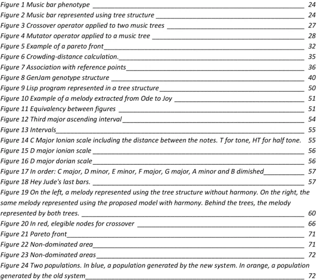
2.1.6.2 Crossover

The aim of the crossover operator is to combine different genotypes in order to produce new genotypes. The crossover operator is usually implemented using two parents which produce two new individuals.

The parents chosen for the operator may be selected randomly or by given a higher probability to be chosen to those with the best score.

The crossover operator can have some difficulties due to its ease to produce invalid individuals. When implemented, some rules must be implemented as well, so the possibility to produce an invalid individual is reduced to zero.

Figure 3 Crossover operator applied to two music trees

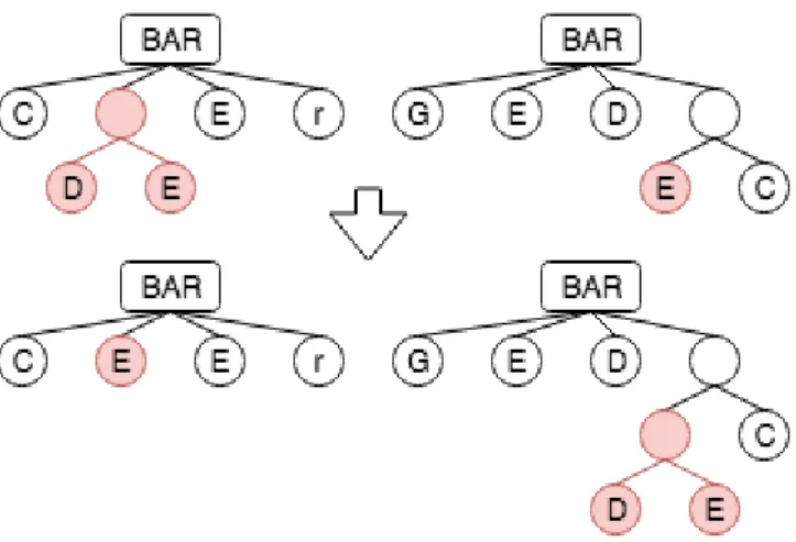
2.1.6.2 Mutation

The objective of the mutator operator is to introduce random changes into a genotype in order to enrich the variability of the population.

When applying the selection and the crossover operator, it is easy to remove potentially useful genotypes, this can be solved with the mutation operator. It can be easily understood with an example.

we use the selection and the crossover operators but it is possible that the mutator operator introduces a random 1 into one of the previous genotypes.

Figure 4 Mutator operator applied to a music tree

2.2 Program flow

The first thing that we need to define in genetics programming is the size of the population. This is the number of individuals that can fit in a population, in every iteration, there must be always the same number of individuals.

After defining the number of individuals, we need to define the number of iterations for the algorithm. In every iteration, a new generation will be generated by applying the genetics operator to the previous population.

Once we have defined those two variables, we can start. The first thing to do is to generate the first population. This population can be initialized randomly or using some predefined rules which can help our algorithm to solve the problem.

Every time we produce a new genotype, its corresponding phenotype must be evaluated by the fitness function. The score achieved by the function will be important for the genetics operators to decide the next step. Having evaluated every individual, we will have produced the mating pool.

Koza proposes in his book to start using the crossover operator. This will double the size of the population. After applying it, a new set is generated with size doubled.

Secondly, we can apply the selection operator. Not all of the individuals of the mating pool will be present on the next population. Every individual is provided by a probability

𝑓(𝑖𝑛𝑑𝑖𝑣𝑖𝑑𝑢𝑎𝑙_𝑛)

∑𝑀 𝑓(𝑖𝑛𝑑𝑖𝑣𝑖𝑑𝑢𝑎𝑙)

𝑖=0

Equation 1 Koza´s formula to calculate the probability of being selected by the environment selection

Being M the size of the mating pool and f(individual) the fitness function result for the given individual. This can be applied if there is only one fitness function.

Finally, we can apply the mutation operation to the individuals selected to the next generation. The result of applying the three operators is considered the next generation. The individual with the highest score on the last generation can be considered the best solution to the proposed problem but the other individuals may not be discarded as they can be good solutions as well.

3. The Multi-Objective Optimization

Problem

One of the problems present in genetics programming appears when there is more than one fitness function used to evaluate the individuals. Choosing the best one may be a difficult task if there is not a defined criterion for it.

In order to introduce this problem, let’s consider two fitness functions, A and B and three individuals, ind1, ind2 and ind3. These are the fitness calculated for the three individuals:

A B

Ind1 1 0

Ind2 0.5 0.5

Ind3 0 1

Table 1 Sample fitnesses

For this example, the best score for both functions is zero. Which of these three individuals is the best? There must be different answers to this question. If we consider that the best solution is the one with the highest sum of scores (5), the three individuals are valid. This approach called ‘linear aggregation’ was very popular when the firsts algorithms were developed.

Other possibility is to use the lexicographic ordering which consists of prioritise one objective and optimising it. Secondly, another objective is prioritised and optimized without degrading the first objective and without taking into consideration the other objectives.

If we decide to calculate the distance to the optimal point, in this case (0, 0), ind2 has a score of 0.71 which is better than ind1 and ind3 as they are at a distance of 1 point. Another possibility can be to choose those individuals with the highest score in each single function, in this case ind1 is the winner for function A and ind3 for function B. As you may see, depending on the approach used to select individuals, the result may vary. This problem is even more difficult if the functions produce different set of scores and the maximum or minimum score is unknown. For the following example, consider that the higher the score is, the better.

A B

Ind1 80 0.3

Ind2 55 0.9

Ind3 70 0.2

Table 2 Not normalised fitnesses

In this case, the differences are too significant, and they cannot be ignored. If we decide to select the sum for example, the fitness B will be almost ignored as it does not have enough weight to change the result of the sum. This fact can produce that the genetics algorithm will prioritize the solutions that fit A and not B.

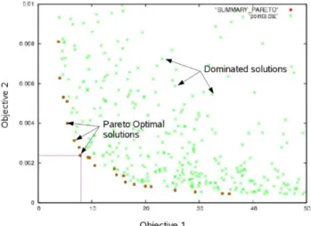
3.1 Pareto front

The pareto front is a representation of the non-dominated solutions. A non-dominated solution, or pareto optimal is the one whose score cannot be improved without degrading the result of the other objectives.

Figure 5 Example of a pareto front1

There are several ways of calculating the pareto front and the algorithm for it depends on the number of dimensions chosen. One easy way of calculating the pareto front for 2 dimensions is sorting one of the objectives in ascending order. Then, the individuals are iterated.

The first individual is added to the pareto front as it is the first optimal individual found, then, the following individual is compared with the last individual added to the optimal individual list, if its second objective is lower than the last added, it is added to the optimal list, otherwise it is discarded.

3.2 Multi-Objective Evolutionary Algorithm (MOEA)

With the aim to solve this problem, some algorithms have been developed even though this problem has not a trivial solution. A multi-objective optimization algorithm must include two important characteristics in order to be considered a good approach.

Firstly, a MOEA must increase the overall score of an individual, this means that it must try to increase all the possible objectives functions available. This have been pursued since the first MOEAs came with different mechanisms (5).

One of those mechanisms that may result interesting to consider is elitisms. Elitism is based on having a different set of individuals with the best traits, used within the crossover operator in order to increase the score of the population.

This set can be a predefined one with manually selected individuals or it can be just the set of the nondominated individuals of the population.

Elitism is an interesting technique that must be considered but using it on music composition can be dangerous. It may seem a good idea to have a second set with human composed songs that may transfer their characteristics to new sets, but the result can be counterproductive due to the probabilities of producing a plagiarised song.

Secondly, a MOEA must keep the diversity of the population. This is called niching. The following section explains several niching methods.

3.2.1 Niching methods

The main reason of niching is to avoid that all the solutions tend to the same point. With the aim of increasing the entropy of a population, the MOEAs have develop several methods for this task.

3.2.1.1 Fitness sharing

Fitness sharing (6) is one of the first niching method developed. It consists of modifying the overall fitness of an individual depending on how crowded the area is where the individual is. The winner out of two individuals with similar scores is the one with less neighbour around.

Fitness sharing decreases the fitness of an individual if it finds individuals with similar characteristics.

3.2.1.2 Crowding

Crowding technique has several different implementations (7) but its first idea is to replace individuals. The author Dejong (8) implemented crowding by selecting an individual and a subset of individuals, the most similar individual of the subset is replaced with the individual selected.

3.2.1.3 Crowding distance

The MOEA NSGA-II (9) implemented a new niching method which consisted on calculating what they call the crowding distance. The crowding distance is the result of

NSGA-II implements a crowded-comparison operator that guides the selection process. The operator uses two values in order to compare individuals, one is the crowding distance explained before and the other one is the nondomination rank which corresponds to the number of individuals that dominate the individual.

The operator uses this algorithm in order to compare two individuals i and j, being irank

the nondomination rank of the individual and idistance the crowding distance.

i is better than j if (irank < jrank) or ((irank = jrank) and (idistance > jdistance))

In other words, if one individual is better than other, it is selected, in case that both are equal, the crowding distance oversees defining which is better.

Figure 6 Crowding-distance calculation.

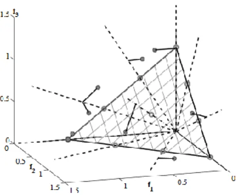
3.2.1.4 Reference point

Reference-point method (10) is based on calculating a set of points in the hyperplane. Every individual is associated with a reference point based on the perpendicular distance between the individual score and the line formed using the reference point and the most optimal point.

Finally, an individual is chosen for each reference point based on the closest distance to the reference line.

Figure 7 Association with reference points

3.3 NSGA-III

Choosing an algorithm to implement for this problem has been difficult. There are several MOEA whose results are attractive but with different results. Some MOEA may ensure that the average solutions for a problem are better than using other algorithm but it may lack some diversity, others may keep diversity but the average score of a population is not as optimal as others.

The NSGA-III algorithm (10), also called NSGA-II with reference-point based non-dominated sorting, it is a relatively recent algorithm that presents better results than its predecessor NSGA-II.

NSGA-III is an improved version of its predecessor, but it changes the niching method used, the crowding distance. NSGA-III uses the reference-point technique instead. For this reason, some authors do not consider NSGA-III as a new version of NSGA.

One of the disadvantages that may be mentioned of using NSGA-III is that we do not have the possibility to define the exact size of the population. The size of the population is computed using the following formula:

𝐻 = (𝑀 + 𝑝 − 1

M is the number of objectives and p the number of divisions. H is the number of reference point used in the algorithm and as we mentioned before, the solution chooses one individual for each reference point.

The NSGA-III algorithm will be implemented as the multi-objective optimization function of our genetic programming framework.

4. State of the Art

This project is based on a wide area that has been previously researched so there are some proposals done before that need to be taken into consideration before starting to develop this project.

4.1 State of the art in computer generated music

There are several pieces of software trying to emulate a human composing music and the approaches used for it are different. There are some programs that use deep learning like

deepJazz (11) or Markov’s chains like JazzML (12). We are going to analyse three different projects that use genetic programming, genJam (13), vox populi (14) and one based on conceptual blending (15).

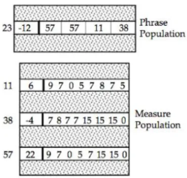
4.1.1 GenJam

GenJam, or Genetic Jammer, is a software developed in 1993 (13) but its algorithm and code have been improved through the years. It is based on a genetic algorithm that is able to compose music without human supervision.

One of the main characteristics of GenJam is that it uses two different populations, one for the measures and the other for the phrases. A phrase is just a set of measures. The purpose of working this way is to reuse measures that have a good fitness score many times.

One of the disadvantages of GenJam is its limitations. For example, it always uses a 4/4 measure and it can only represent 14 notes due to definition of its chromosome representation. It uses a string for it.

Figure 8 GenJam genotype structure

This is an example of a genotype. The first number on the left of the box it is just the index of the element, in this case we have the 23th phrase of the population. The following number isolated in a box is the fitness achieved, in this example, this phrase has a negative punctuation because it is not considered a good phrase chromosome. The following numbers are pointers to measures.

The measure structure has an index and a fitness as well but the meaning of the numbers on the right is different. If it is a 0, it represents a rest on the melody, between 1 and 14 is a pitch and 15 is a hold which means that it continues playing the previous note.

As you may notice, the genotype is designed to be optimal. The size of the population, the individual and even the characteristics of the individual are powers of two. This is a limitation of the time when the algorithm was developed.

4.1.2 Vox Populi

Vox Populi uses genetic programming to evolve a set of chords. Chords are represented using a 28-bit binary string and each note of the chord is represented in a 7-bit binary string.

The genetic operators cross the chords in order to produce new ones. The fitness criteria used is the melodic fitness, the harmonic fitness and a voice range fitness.

4.1.3 Conceptual blending

The author Kaliakatsos-Papakostas (15) proposed a new approach for generating drum rhythms based on conceptual blending as a way of creating new styles.

The methodology used by his project is the following one:

Firstly, two rhythms are chosen by a human as input. For both rhythms, 32 features are extracted. The features of both rhythms are blended, creating a new vector of features which include the most important features of each rhythm.

Secondly, a genetic algorithm is used within the vector of features created on the previous step. The initial population includes an equal number of copies of the two original rhythms.

The genotype structure is a 2-dimensional array with 3 rows, each row represents a basic drum and 12 to 24 columns which correspond with the number of beats.

The genetic evolution used implements fourth different crossover operators that apply different set of operations to the genotype.

4.2 State of the art in evolutionary computation

libraries

There are plenty of evolutionary computation libraries for general purposes. They allow the user to define a set of rules on its genotype so they can slightly adapt themselves for every problem proposed and they implement different algorithms that may be useful in order to sort a determined obstacle. I am going to focus on java libraries due to the fact that is the language used in this project.

4.2.1 JMetal

JMetal (16) is not an evolutionary computation library itself but it provides a set of multi-objective and single-multi-objective algorithms that are necessary on genetics. These algorithms help us to select the best individuals that fit better in our environment. Some of those algorithms are NSGA-II, MOEA/D, MOCell…

In order to test those algorithms, JMetal provides a set of problems that can be used as a benchmark. Ones of those benchmarks are provided by the DTLZ test suite.

The DTLZ suit (17) provides seven problems with box-constraints that can be optimized with a variable length of fitness functions, due to this, its problems are perfect for testing. One of the problems is DTLZ1 (17), whose solutions are those that are located on a linear hyperplane on 0.5.

JMetal can work mainly with binary or string chromosome representations.

4.2.2 Jenetics

Jenetics (18) is a genetic library for java that uses mostly trees for the genotype representation. It allows the user to use trees, parenthesis trees and flat trees as the input for the population.

The multi-objective optimization algorithm used by Jenetics is NSGA-II so we can consider that Jenetics lacks multi-objective optimization algorithms as there are better options than that algorithm.

Other advantages presented in ECJ is that it supports different genotype representations. It uses its own tree representation and provides the user a syntax to define the requirements of a valid tree for the problem.

The other main representation is the vector. It can use fixed-length vectors and variable ones.

In order to test performance, ECJ provides a set of problems that can be used for testing, for example, the performance of two different multi-objective optimization algorithm. There are some problems that use vector representation and other that use trees instead. Another feature of ECJ is that it implements the flyweight pattern which is able to save computer resources while solving a problem by abstracting the common characteristics of the individuals in a population.

5. Technologies and Methodology

Choosing the technologies for this project has been easy due to the fact that this project continues an existing project so some of the tools used are inherited. In this chapter, we will provide a short description for the tools used in this project and the methodology used to fulfil the requirements.

5.1 Technologies

5.1.1 Java

Java is a compiled general-purpose language programming language. It is compiled to bytecode which is interpreted by the Java Virtual Machine. Due to this, java can run on every operating system able to run the Java Virtual Machine such as Windows, MacOS and Linux distributions.

Java is widely use due to its power and ability to be portable to every system. It has one of the largest communities and according to stackoverflow (20) is the second most loved programming language in 2019.

The java version used for the project is Java SE 8 because is a long-term support version. Even though java has a lot of advantages, it has been criticised for being a high resource consuming language.

We have used java because it is the language programming used on the original project.

5.1.2 Eclipse

Eclipse is the IDE chosen for Java. Eclipse is open source and it is supported by the Eclipse Foundation. It provides different versions for several programming languages

The advantages of using eclipse are that it provides a full environment with powerful tools that increase the productivity when working with java.

Other reason for using eclipse is that the original project is an eclipse based project and migrating it can be a difficult task that may be not part of this project.

5.1.3 GIT

Git is a version-control system that will help us to control our code. We have used github.com for storing our remote git repository.

Git has help us providing some tools to control the changes produced in the code.

5.1.4 Visual Studio

In one step of this project, we will need to work with a project written in C++, for this task we have chosen Visual Studio as our IDE.

Visual Studio is an IDE developed by Microsoft which can work with C++, C# and F# among others. The main reason for choosing this IDE was the powerful debugger integrated that has helped us to understand how the C++ project was developed.

5.2 Methodology

We have divided our project in two different objectives, one is implementing our own genetic programming library and the other is changing the data model used in our problem. For this reason, we have defined two goals.

After that, we have defined several requirements for our both goals. Both goals have followed these steps: research, implementation and testing.

6. Data Model

The structure selected for the chromosome representation in this problem is the tree data structure. This structure was firstly proposed by Koza in its book genetic programming (3) but the rules in which the actual model for the problem is based and the original ones differ.

In this chapter, we will explain why was proposed the tree as an excellent approach for genetic problems representations, how is implemented for music composition and how can it be improved.

6.1 Koza tree structures

Koza proposed that genetic programming was a valid strategy for solving problem whose solution was not trivial. When Koza refers to a solution to a problem, he may refer sometimes to a set of variables that may be the solution itself or sometimes to a program which is able to solve a problem by defining a set of parameters as an input.

This second approach is basically a computer program and this idea can have tons of difficulties. The proposed language for this task was Lisp.

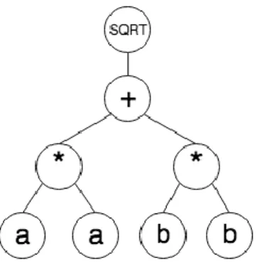
Lisp is a multi-paradigm programming language, but we are going to focus on functional programming paradigm. Let’s consider that finding the formula to find the hypotenuse of a right triangle is not trivial and we want to solve the problem using genetic programming. The solution expected for this problem in lisp is the following one, we have omitted the possibility to use the power function in order to give a better example:

(sqrt (+ (* a a) (* b b)))

The advantages of using Lisp is that its syntax can be easily represented as tree. The code explained before can be translated to the following tree:

Figure 9 Lisp program represented in a tree structure

This representation can be used in genetic programming due to the fact that defining a set of rules ensures that it can be changed randomly but the result will produce another valid program with a valid syntax.

One example of rule that ensures the tree as valid is that a SQRT node can only have one child, if we disobey this rule, we can produce a Lisp program that may led to a compiling error.

6.2 Music tree model

The model used by the GRFIA application (2) is a good way to represent a music melody as it gives the possibility of changing the structure of the melody without breaking the metric rules used in music.

On the contrary to the Lisp tree models, the nodes used in this structure may be only valid on a fixed level and using them on a different level may led into an invalid tree structure. We will explain some music theory with the aim of explaining some of the rules followed by this model.

The tree structure represents a whole melody. A melody is a combination of pitch and rhythm. The rhythm of a melody is expressed using a meter signature and every melody must have one.

Figure 10 Example of a melody extracted from Ode to Joy

In this example, the meter signature is 4/4. It is defined by a numerator and a denominator and they have a different meaning depending on if the measure is simple or compound. We will simplify the problem using only simple measures.

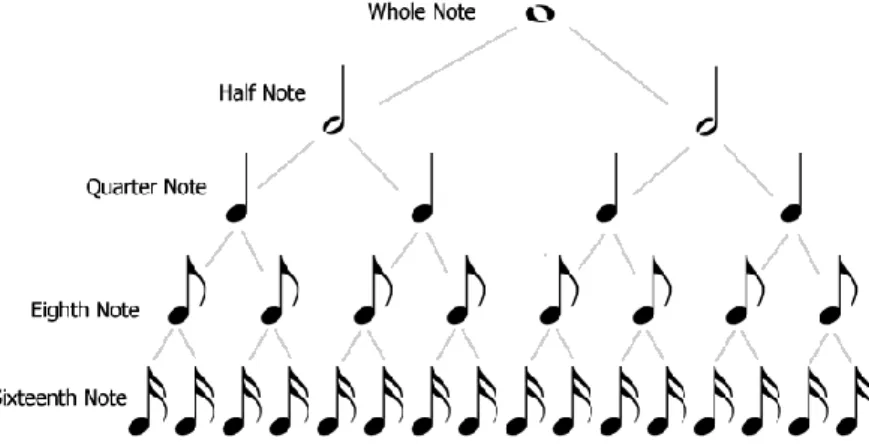
The denominator of a simple time meter indicates the note value that fulfils one beat in a bar. This value is always a power of two because it is calculated by dividing the whole note whose value is 1, then the half note is 2, quarter note 4 and so long.

On the other hand, the numerator indicates the number of beats that fill a measure. Every measure must be filled with all the beats that can fit on it.

Applying these rules to the example showed before, the 4/4 time signature means that every of our bars ruled by this metric will have 4 beats with a quarter note on each beat. This does not mean that we need to use always 4 quarter notes, we can use every combination of notes that fit on that bar, so for example a single whole note or 8 eighth notes can be valid bars.

Figure 11 Equivalency between figures

Secondly, we have the pitches of the melody. A pitch is a sound that is played on a specific frequency. In order to represent a pitch, we need two elements, a staff and a clef. The key indicates where is located a reference pitch, for example, the clef most used is the G-clef or treble clef which indicates that the fourth G of the piano is represented in the second line of the staff.

There are seven different pitches and after the seventh pitch, the sequence starts again with the first pitch. Those seven pitches are C, D, E, F, G, A and B. If we want to know the frequency of a pitch, we need to know the octave of it. So, for example, the A pitch on the fourth octave represents the frequency 440hz, the A pitch on the next octave represents 880hz.

Summing up, in one hand we have that in order to represent a pitch we need to know its name and its octave and on the other we have that in order to represent that pitch in a music score, we need a staff and a clef.

The distance between pitches is calculated using tones. There are some intermediate pitches and they can be represented using accidentals. The sharp accidental adds half tone to a pitch and the bemol subtracts half tone. If we take into consideration those intermediate pitches and we represent them using sharps, the list of pitches will be C, C#, D, D#, E, F, F#, G, G#, A, A# and B, 11 in total.

Having explained how a melody is defined, we can then explain how this can be translated into a tree.

The tree starts we a root node, the root node does not contain music information. Then, the children of the root nodes are the sections. Sections are not compulsory, and they are not in music theory, but they can help to organise the structure of the melody. Sections are used in some music pieces, for example the sonata is divided in three sections and sometimes it follows an A B A structure.

The children of the sections, in other words, those on the third level of the tree, contain measure labels. The measure label contains the time signature. Every measure node is translated to a bar in a music score.

If we remember, the numerator indicates the number of beats that fill a bar and the denominator indicates the value of each beat. The numerator is translated to the tree indicating the number of children that the measure node must have and the denominator the value of each beat.

The child of a measure label can have 4 different labels:

- Pitch label: A label containing a pitch and the octave of the pitch.

- Continuation label: This label means that the beat keeps playing the previous played sound. In music, this can be represented using longer notes, dotted notes and ties.

- Rest: This is translated as a silence in a music melody.

- Empty label: We use this label to indicate that this is not a leaf node.

If we use an empty label, the node container must have two children, this is because the duration of that beat is divided in two parts. So, for example, if we have a node that represents a quarter note and we want two have two eighth notes, we will put an empty label on the node and two children that will represent each eighth note.

As we can notice, melodic information is stored in the labels contained by the nodes and the rhythm information is decided by the structure of the tree.

There is another advantage of this model and it is the possibility to store this data in string form as a way to store the model if needed. Translating this tree to a nested parenthesis is easy, the possible labels for this are:

Root: Corresponds to the root of the tree. S: It means section.

M: For the measure label, it translates to a whole bar.

^: Empty label, for those levels that need to be divided in two sub beats. -: Represents the rest.

.: Continuation, it can be translated to a dotted note or a tie.

A, B, C, D, E, F, G: Represents a pitch, it needs an integer to represent the octave of this pitch.

6.3 Adding harmony information to the music tree

As we introduced in this document, one of the aims of this project is to try to improve the model utilised for representing music melodies. This is going to be done by changing the way it works and the way it is translated to a music score but before we can introduce this change, we need to explain what harmony is.

As we described before, a melody is a set of notes played sequentially with the aim of producing a sound that may sound appealing to the listener. These notes can be any notes but if we want to produce better melodies, we need take into account the rules of harmony. Harmony provides a set of rules that may identify pitches that played together or one after another should sound nice to the listener. The main tool in harmony are chords but we need to introduce a few concepts before.

6.3.1 Intervals

If we take two different notes and we analyse the distance between the two different pitches, we are talking about an interval. The characteristics needed to fully identify an interval are the name of the both pitches, the distance between them and if the distance is ascending or descending.

Figure 12 Third major ascending interval

An interval can be perfect, major, minor, augmented and diminished. These names may also define how will be the sound when both pitches are played. A perfect interval produces a neutral sound, a major produces a happy sound while minor intervals produce

An interval is perfect when we the distance between two pitches is 4, 5 or 8 pitches and they have between them 5 semitones, 7 semitones and 12 semitones each.

Intervals with 2, 3, 6 or 7 pitches of distance are major when they have 2 semitones, 4, 9 and 11 semitones each. For the same intervals, if we remove one semitone, we will produce the equivalent interval in minor mode.

If we add a semitone to a major interval or a perfect interval, we will have an augmented interval, if we add two a double augmented interval and so long.

If we remove a semitone from a minor interval or a perfect interval, we will produce a diminished interval, if we remove two then double diminished as augmented intervals.

Figure 13 Intervals

6.3.2 Scales

A scale is an ordered set of notes built using a formula. In order to simplify the explanation, we will focus on the common scales. In order to build a scale, we need a pitch, this pitch is going to be the first one of the pitches set. Secondly, we need a key, this can be major or minor and finally we need a mode, the mode depends on the key, so we are going to use de major key for this task.

The most basic scale that we can built is the C major Ionian scale.

Figure 14 C Major Ionian scale including the distance between the notes. T for tone, HT for half tone.

The formula used to produce this scale is the following one, where the interval indicated is the one between the first pitch and the current pitch:

If we change the first note of the set and recalculate the other pitches, we will produce a different scale so for example, if we have D as a reference pitch and we want to produce D major Ionian, this will be the result:

Figure 15 D major ionian scale

If we produce an Ionian scale and then we shift the set, we will produce the following mode. So, for example, if we take the ionian scale and then we shift the set to the left one position, the resulting set is the D major dorian scale:

Figure 16 D major dorian scale

The major modes are Ionian, Dorian, Phrygian, Lydian, Mixolydian, Aeolian and Locrian.

6.3.3 Chords

A chord is the combination of three or more pitches. Chords are similar to scales; they need a reference pitch and a formula. The easiest way to generate a chord is using a scale. Let’s use the C major Ionian scale for this example. If we take the first, third and fifth pitches of the scale, we will produce the C major chord. The major chord is generated by using these intervals:

1º Perfect, 3º Major and 5º Perfect

You may notice that these intervals are part of the major Ionian scale. If we have a scale with seven pitches, every pitch will generate a chord. These chords are named using

I, ii, iii, IV, V, vi, viiº Or using names:

C major chord, D minor chord, E minor chord, F major chord, G major chord, A minor chord and B diminished chord.

Figure 17 In order: C major, D minor, E minor, F major, G major, A minor and B dimished

Depending on the scale, it may produce other different basic chords, but we are not going to include them here.

One easy way to recognise the scale of a song is checking the first and last pitch of it. This method does not always work but it may be helpful sometimes. If the starting pitch is different to the last, the last pitch has priority over the first. Let’s use the song Hey Jude

from The Beatles as an example, the starting pitch is G and the last pitch is C, so C has more probabilities to be the reference pitch of the scale. Secondly, we need to know if it is major or minor, this is can be discovered checking the key signature. The key signature is a set of bemols, or sharps located on the left of the clef of the score.

The key signature of a scale is calculated counting the number of bemols or sharps necessaries to represent the scale, for example the C major scale needs 0 accidentals, but G major scale needs one. The order of the accidentals is logically ordered using music theory, if the scale uses sharps, the first sharp is F#, then C#, G#, D#, A#, E#, B# and then after B#, it will repeat and be F## and so long so far. The order of bemols is Bb, Eb, Ab, Db, Gb, Cb and Fb.

Retaking the Hey Jude example, we knew that the first degree of the scale was C but we did not know it was major or minor. The key signature has 0 accidentals and C minor needs 3 bemols but C major needs 0 so the probabilities that the scale of this song is C major are very high.

6.3.4 Chord progressions

When a music piece is being composed, one of the first thing decided is the scale. Having decided the scale for the song, then a chord progression is chosen using the possible chords of that scale.

So, let’s consider that we are composing a song in C Ionian major, C major from now on. The possible chords of this scale are C major (I), D minor (ii), E minor (iii), F major (IV), G major (V), A minor (vi) and B diminished (viiº).

Using those chords is not compulsory and we can even make some modifications. A valid progression can be I V vi IV but for example we can add the a 7º interval to the iv chord, if we do that, we will have the progression I V vi7 IV. The progression used for this example is the one of the most common used in pop music, some examples can be Let it be from The Beatles, Forever Young from Alphaville or Take on me from A-ha (21). Chord progression has been always a good way to identify music genres, it can be used for example to distinguish between a jazz song and a blues one.

When using a chord progression, it is not compulsory to use all the notes that conform the chord and it is very likely that other pitches from the scale’s chord are used for the melody.

6.4 The improved tree model

Having introduced some harmony concepts, now is easier to identify which elements are necessary for a genotype that can store them.

One of the first thing that we need is a scale. This scale will be used for the whole melody so the best place for it is in the root node of the melody as it defines what is coming on

Secondly, we need a chord progression. It is very typical to have different chord progressions inside a melody, for example in pop music, the progression used for the chorus can be different to the one used in the bridge.

The best way we have found to store this information is using the sections nodes. This is helpful because we can use sections to delimitate progressions. Some sections used in western modern songs are the bridge, the chorus and the pre-chorus.

Every measure node, child of a section, will use one of the chords stablished on the section node. The way is decided is by calculating the module of the number of measure nodes divided by the number of chords in the progression. So, if we have a three chord progression, the fourth bar of that section will use the first chord of the progression. Building a tree with a root node without scale or a section node without chords will produce an invalid tree.

Finally, we have the leaf nodes, those that must be after the measure nodes. The leaves representing rests and continuations stay as the original tree model, but the ones used to represent pitches are not used anymore in this model, we use degree labels instead. As we said, every bar has a defined chord, but the pitches used in that bar can be any contained in the scale used to generate the chord. The chord is used in order to define the probability to find a degree in a bar.

There are 7 possible degrees and an octave is needed as well in order to know the frequency of that pitch.

Figure 19 On the left, a melody represented using the tree structure without harmony. On the right, the same melody represented using the proposed model with harmony. Behind the trees, the melody represented by both

7. Implementing the Library

7.1 Implementing the selection operator

One important question that considers this project is why not using a java library that implements this algorithm and the answer for it is that an own implementation gives us the freedom to change whatever is needed.

This may be important as one of the proposed future tasks raises the need of changing the way NSGA-III works.

We are going to use NSGA-III as our multi-objective optimization algorithm, and it will be in charge of the environmental selection.

Another reason for this implementation is performance. The problem of using a general-purpose library is that we have to adapt our problem to the data model used by the library. One example is our program, for every population, it needs to convert the music tree model into the tree used by the library, then the tree is converted back to the music tree model until the next generation. Having our own implementation has given us the possibility to use our own model.

7.1.1 Step 1: learning how it works

Implementing an algorithm from scratch may be a difficult task due to its mathematical complexity. For this reason, we have decided to base our implementation in one C++ implementation (22).

This implementation has been used by libraries like JMetal in order to implement NSGA-III (23) so we can consider it as a good example to start.

The example program implements several problems used for testing purpose. Those problems are from the DTLZ collection, they are based on mathematical problems that use an array of numbers as a genotype.

Having debugged it a few times we can get some conclusions:

- The selection algorithm does not depend on the genotype type.

- The only information needed on the selection state is the fitness of each individual.

- The crossover and mutator operator depend on the genotype structure. - There is a problem that stores possible constraints for our problem.

Moreover, there is a math class that stores a function that calls the C++ random number generator. We will replace this function with our own generator in order to be able to generate the same numbers on java and C++ for testing purposes.

We have chosen the DTLZ1 problem in order to understand how the algorithm works because it is simple and easy to understand.

The C++ program uses a param file in order to load some configuration values: - Name: The name of the problem, it does not have any important use.

- Obj_division_p: As we explained before, the algorithm NSGA-III needs one parameter in order to work and this is the entry parameter for it.

- Gen_num: It defines the number of generations for the genetic algorithm. - Crossover_rate: Defines the possibility of two individuals getting

crossovered.

- Crossover_eta and Mutation_eta: These values define how do these operators affect to the individuals. The lower the eta is, the more different are the individuals affected.

The configuration parameters that are provided with a config file are not going to be used anymore because they can be configured using the GUI of our software, so we are going to replace them with getters and setters in the future.

The entry point of the algorithm will have a method that receives a problem which contains the problem constraints and the fitness functions.

The individual object will store mainly the genotype of the individual and the scores provided by the fitness functions.

Firstly, the reference points that is going to use later are generated. It takes two arguments, the number of divisions and the number of objectives to optimized that is provided within the problem. The reference point stores its coordinates in a variable length vector. Secondly, the first generation is constructed, every individual is evaluated by the objective functions.

Thirdly, it starts an iterative loop that run once for every generation. The first thing done by the loop is to apply the crossover operator, it chooses two random parents used for producing two new individuals. Those individuals are then mutated by the mutator operator and finally, the result of the mutation is evaluated in order to include their fitness. Fourthly, after finishing the crossover and mutation step, the environment selection is executed. This step is the most difficult part of the program as it keeps all the multi-objective optimization algorithm’s logic.

The NSGA-III algorithm starts calculating the fronts. Fronts are subsets of individuals. Those individuals found on the first front are those that are not dominated by any other individual, like the pareto front. The second front is made up with those individuals that are not dominated by any individual except for those found on the first front and so long. Once we have computed the fronts, we only need to have as many individuals as the population size, it must be mentioned that, even though we have doubled the population size during the crossover, we need to keep the initial size.

We only need to use the number of fronts needed to keep the population size. For example, if we are running the algorithm with 100 individuals, after the crossover we

60 individuals, the second one 70 and the last one 80, we do not need the third front anymore as we can keep 100 individuals just using the first and the second front.

If the number of individuals is exactly the population size, the environmental selection is finished as we can ensure that those individuals are the best, otherwise, we need to continue with the algorithm.

The following step is computing the ideal point using the best coordinates found on the population, so for example, if we are trying to minimise the score and we have two objectives and two individuals with fitness (10, 7) and (8, 11), the ideal point is (8, 7). After that, we need to convert the objectives by subtracting the ideal point to every individual, for the previous example, the fitness (10, 7) is converted to (2, 0).

After computing the ideal point, we need to calculate the extreme points, which are those with the worst score.

Once we have the ideal point and the extreme points, we can calculate the reference points. In order to calculate the reference points, we need to build a hyperplane using the extreme points calculated before and then, intercept the lines formed by the reference points calculated on the first step of the algorithm and the ideal point.

Every individual must be associated with a reference point. For every individual, it is calculated the distance between the individual and the reference line, the one formed using the optimal point and a reference point. The individual is associated with the closest line found.

It is possible to find reference points without any individual associated. In this case, the reference point is excluded and is not taking into consideration in this generation.

Finally, the next population is built. Those reference points with the minimal cluster size are chosen, if there is a draw, a random reference point is chosen. Then, the best individual associated with the reference point is selected, added to the next population and deleted from the possible reference point’s associated individuals list.

7.1.4 Step 3: testing

The algorithm has been testing using the DTLZ1 algorithm. We have replaced the random number generator used by the implementation in C++ and the implementation in Java. After the execution, we have compared and checked that the result was the same.

7.1.5 Step 4: refactoring the code

Having ported and tested the algorithm, now we have a library able to optimize multi objective problems, but it still has a problem, it can only be used with the array of numbers genotype structure.

In order to give the algorithm, the ability to work with different genotypes, we need to identify those parts that depends on the genotype structure and extract them from the algorithm itself. This task is going to be done using two important tools: interfaces and generics.

We can define three parts that depends on the genotype:

- The initializer: one of the first steps of the algorithm is initialising the first population.

- The crossover: depending on the structure of the genotype, the crossover operator will perform different actions.

- The mutator: as the crossover operator, it needs to know the structure of the genotype in order to change it.

We are going to use generics in order to keep constraints.

7.2 Implementing the crossover operator

are going to use only those nodes whose parents or the parents of their parents are bars, excluding the root node, the section nodes and the bar nodes, this will help us to increase diversity of the population.

Firstly, two individuals are chosen randomly, and their eligible nodes are counted.

Figure 20 In red, elegible nodes for crossover

Secondly, two random numbers are generated between 1 and the node count. The N node found in pre-order search is selected as the node to be crossed.

Finally, the selected nodes are swapped generating two new individuals. If this combination produces an invalid tree that exceeds the max tree depth, the parent of the node is selected instead for this swap until it produces a valid tree.

There is a parameter that specifies the possibility of crossover between two individuals called the crossover rate.

7.3 Implementing the mutator

Implementing the mutator operator has the same difficulties as the crossover operator, we need to avoid invalid trees. In this case, it is easier to avoid these problems. There is a parameter that specifies the chances of one individual being mutated and it is called the mutation rate.