Interfacing The CFD Code MFiX With The PETSc Linear Solver Library To Achieve Reduced Computation Times

(1)

University of North Dakota

UND Scholarly Commons

Theses and Dissertations Theses, Dissertations, and Senior Projects

January 2018

Interfacing The CFD Code MFiX With The PETSc

Linear Solver Library To Achieve Reduced

Computation Times

Lauren Clarke

Follow this and additional works at:https://commons.und.edu/theses

This Thesis is brought to you for free and open access by the Theses, Dissertations, and Senior Projects at UND Scholarly Commons. It has been accepted for inclusion in Theses and Dissertations by an authorized administrator of UND Scholarly Commons. For more information, please contact

Recommended Citation

Clarke, Lauren, "Interfacing The CFD Code MFiX With The PETSc Linear Solver Library To Achieve Reduced Computation Times" (2018).Theses and Dissertations. 2189.

(2)

INTERFACING THE CFD CODE MFIX WITH THE PETSC LINEAR SOLVER LIBRARY TO ACHIEVE REDUCED COMPUTATION TIMES

by

Lauren Elizabeth Clarke

Bachelor of Science, University of North Dakota, 2016

A Thesis

Submitted to the Graduate Faculty of the

University of North Dakota

In partial fulfillment of the requirements

for the degree of Master of Science

Grand Forks, North Dakota May

(3)

(4)

(5)

PERMISSION

Title: Interfacing the CFD Code MFiX with the PETSc Linear Solver Library

to Achieve Reduced Computation Times

Department: Chemical Engineering

Degree: Master of Science

In presenting this thesis in partial fulfillment of the requirements for a graduate degree from the University of North Dakota, I agree that the library of this University shall make it freely available for inspection. I further agree that permission for extensive copying for scholarly purposes may be granted by the professor who supervised my thesis work, or in his absence, by the Chairperson of the department or the dean of the School of Graduate Studies. It is understood that any copying or publication or other use of this thesis or part thereof for financial gain shall not be allowed without my written permission. It is also understood that due recognition shall be given to me and the University of North Dakota in any scholarly use which may be made of any material in my thesis.

Lauren Elizabeth Clarke May 2018

(6)

TABLE OF CONTENTS

LIST OF FIGURES ... viii

LIST OF TABLES... xii

NOMENCLATURE ...xiii ACKNOWLEDGEMENTS ... xvii ABSTRACT ... xviii CHAPTER 1. INTRODUCTION ... 1 1.1 Motivation ... 1 1.2 Objectives ... 3 1.3 Thesis Outline ... 3 2. BACKGROUND ... 5 2.1 Multiphase Flows ... 5 2.2 Two-Fluid Model ... 6

2.3 Partial Differential Equations ... 7

2.3.1 Conservation of Mass ... 7

2.3.2 Conservation of Momentum ... 7

2.3.3 Conservation of Species Mass ... 8

2.3.4 Conservation of Energy ... 9

(7)

2.3.6 MFiX Solution Procedure ...13

2.3.7 Pressure Correction Equation ...17

2.4 Numerical Methods ...18

2.4.1 Linear Algebra ...18

2.4.2 Linear Systems ...23

2.4.3 Iterative Methods ...24

2.4.4 Stationary Iterative Methods ...24

2.4.5 Krylov Subspace Methods ...25

2.4.6 Preconditioning ...27

2.4.7 Convergence ... 30

2.5 Interfacing MFiX with PETSc ... 31

3. BUILDING THE SOFTWARE ...33

3.1 Native MFiX ...33 3.2 Native PETSc ...33 3.3 MFiX-PETSc Interface ...34 3.3.1 leq_petsc.f ...34 3.3.2 solve_lin_eq.f ...35 3.3.1 Makefile ...35

4. 3D, STEADY-STATE HEAT CONDUCTION ...37

4.1 Problem Overview ...37

4.2 Results ...39

(8)

5.1 Problem Overview ...45 5.2 Results ...47 6. 3D FLULIDIZED BED ...58 6.1 Problem Overview ...58 6.2 Results ...59 6.2.1 Glass Particles ...59 6.2.2 Polypropylene Particles ...75

7. 2D FLULIDIZED BED WITH FINE CENTRAL MESHING ...79

7.1 Problem Overview ... 79 7.2 Results ...81 8. SUMMARY...85 8.1 Conclusions ... 85 8.2 Future Work ...87 REFERENCES ...89 APPENDIX ...92

(9)

LIST OF FIGURES

Figure Page

2-1 A multiphase flow system with two solid particle types can be represented

as a two-phase system or a three-phase system with the MFiX-TFM [8] ... 6

2-2 (a) A cube broken down into a 10x10x10 computational mesh, and (b) a

single control volume defined by its node locations in the x-direction [2]...10

2-3 Notation used for node locations in TVD schemes, based on flow direction [2] ...12

2-4 A two-dimensional representation of a control volume on a staggered grid

which is used in the finite volume method for discretizing the transport

equations [10] ...14 2-5 Multiplication of matrix A (2 × 3) with matrix 𝐵 (3 × 2) to get matrix C (2 × 2) ...22

2-6 A 16x16 square matrix distributed across two processors, with each

containing a shaded local diagonal block [18] ...30

4-1 Geometry dimensions and boundary conditions used to carry out the 3D,

steady-state heat conduction case ...37

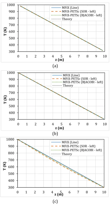
4-2 Temperature distributions in the z-direction when x = 2.25 cm and y = 5 cm

for Cases 1.1 – 1.3 and mesh sizes of (a) 20x20x20, (b) 60x60x60, and

(c) 100x100x100...40

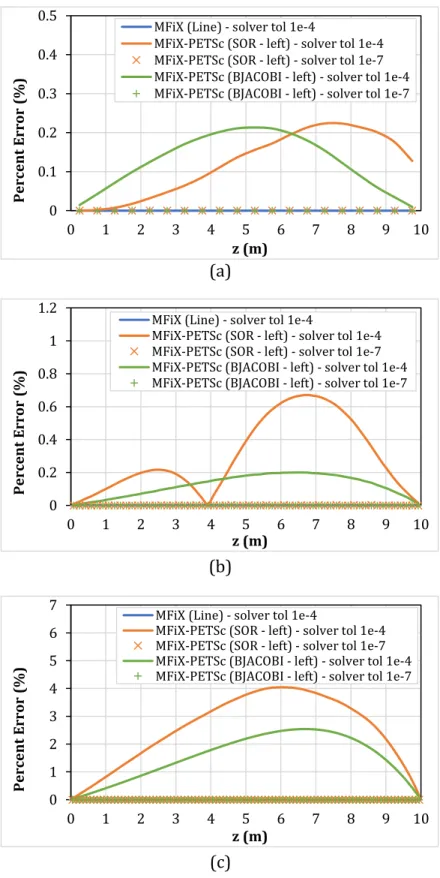
4-3 Percent errors for temperature in the z-direction when x = 2.25 cm and

y = 5 cm for Cases 1.1 – 1.5 and mesh sizes of (a) 20x20x20, (b) 60x60x60,

and (c) 100x100x100 ...42

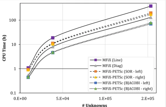
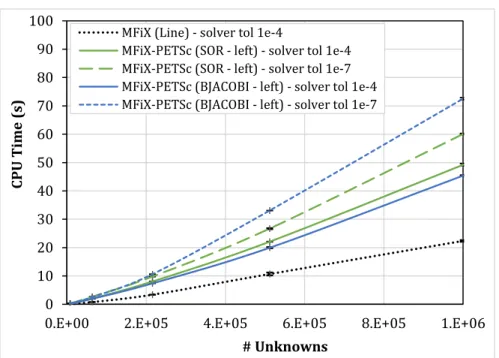
4-4 Comparison of CPU time as a function of problem size for Cases 1.1 – 1.5, with

(10)

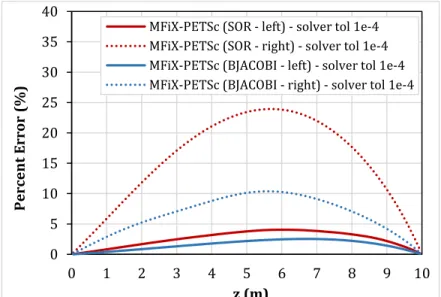
4-5 Comparison of temperature percent errors obtained for Case 1 using left-side (Cases 1.2 and 1.3) and right-side (Cases 1.6 and 1.7) preconditioning in

MFiX-PETSc for an intermediate solver tolerance (10-4_{) and a fine mesh}

(100x100x100) ...44

4-6 Comparison of the CPU time required to solve Case 1 using left-side (Cases

1.2 and 1.3) and right-side (Cases 1.6 and 1.7) preconditioning in MFiX-PETSc

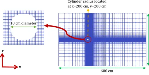
for an intermediate solver tolerance (10-4_{) and a fine mesh (100x100x100) ...44} 5-1 The coarse mesh (120x80) and dimensions used to simulate Case 2 ...46 5-2 Surface points along the cylinder represented as angles ...48

5-3 Comparison of time-averaged pressure coefficients obtained with (a) MFiX’s

line relaxation and (b) MFiX-PETSc’s left-side Block Jacobi preconditioners against experimental measurements from Norberg [20] using a coarse

mesh (Case 2.1) ...49

5-4 Comparison of time-averaged pressure coefficients obtained with (a) MFiX’s

line relaxation and (b) MFiX-PETSc’s left-side Block Jacobi preconditioners against experimental measurements from Norberg [20] using an intermediate mesh (Case 2.2) ...50

5-5 Comparison of the (a) pressure and (b) y-velocity contours between F.O.U.P.

and van Leer discretization schemes at 100 seconds using left-side Block Jacobi preconditioning in MFiX-PETSc and diagonal scaling preconditioning

in the native MFiX solver ...51

5-6 Comparison of time-averaged pressure coefficients obtained in Case 2.3

against previous experimental measurements from Norberg [20] for

F.O.U.P. discretization ...52

Superbee discretization ...53

van Leer discretization ...53

5-9 CPU time as a function of problem size for Case 2 using the F.O.U.P.

(11)

5-10 CPU time as a function of problem size for Case 2 using the Superbee

discretization scheme ...56 5-11 CPU time as a function of problem size for Case 2 using the van Leer

discretization scheme ...56 5-12 Average pressure solver iterations required throughout Cases (a) 2.1, (b) 2.2,

and (c) 2.3 (with standard deviations) ...55 6-1 Dimensions and central jet location of the 3D rectangular fluidized bed ...58

6-2 Comparison of power spectra obtained using (a) left and (b) right

preconditioning in MFiX-PETSc against native MFiX for an outer tolerance of

10-1_{, a solver tolerance of 10}-1_{, and F.O.U.P. discretization (Case 3.1) ...62}

6-5 Comparison of pressure fluctuations for different preconditioners employed

in Case 3.3 which indicates a fluidization regime transition occurred ...65

10-1_{, a solver tolerance of 10}-1_{, and van Leer discretization (Case 3.4) ...67}

6-9 An example of the pressure fluctuations obtained with F.O.U.P. versus van

Leer discretization schemes using the same tolerance levels and

(12)

6-10 CPU time ratios (MFiX-PETSc CPU time / native MFiX CPU time) for (a) F.O.U.P. and (b) van Leer discretization schemes employed throughout Cases

3.1 – 3.6 ...71

6-11 Comparison of the average iterations (with standard deviations) required by each preconditioner-solver combination to solve the pressure-correction equation when (a) F.O.U.P. and (b) van Leer discretization schemes were employed throughout Cases 3.1 – 3.6 ...72

6-12 Comparison of power spectra obtained for Case 3.7, which used a 20 m/s jet...73

6-13 The (a) CPU time ratios and (b) average solver iterations with standards deviations for Case 3.7, which used a 20 m/s jet ...74

6-14 Comparison of power spectra for Cases (a) 4.1 and (b) 4.2 ...76

6-15 CPU time ratios (MFiX-PETSc CPU time / native MFiX CPU time) for Cases 4.1 and 4.2 ...77

6-16 Average solver iterations, with standard deviations, for Cases 4.1 and 4.2 ...78

7-1 Case 5: (a) Dimensions of the rectangular fluidized bed (2D); (b) Mesh size ...79

7-2 Comparison of power spectra obtained for Cases (a) 5.1 and (b) 5.2 ...81

7-3 The (a) CPU time ratios and (b) average number of solver iterations with standard deviations over 10 seconds of fluidized bed simulations (Case 5) ...83

7-4 The (a) number of time steps and (b) number of outer iterations over 10 seconds of fluidized bed simulations (Case 5) ...84

(13)

LIST OF TABLES

Table Page

4-1 Summary of grid dimensions, meshing, tolerances, solvers, and

preconditioners employed in Case 1 ...39

5-1 Summary of grid dimensions, meshing, time steps, tolerances, solvers,

discretization schemes, and preconditioners (P.C.) employed in Case 2 ...47 6-1 List of material properties used for glass particles throughout Case 3 ...59

6-2 Summary of grid dimensions, meshing, time steps, tolerances, inlet velocities,

solvers, discretization schemes, and preconditioners (P.C.) employed in Case 3 ...60

6-3 List of material properties used for polypropylene particles throughout Case 4 ...75

6-4 Summary of inlet velocities, meshing, time steps, tolerances, solvers,

Discretization schemes, and preconditioners (P.C.) employed in Case 4 ...75

7-1 Summary of fluidization materials, meshing, time steps, tolerances, solvers,

(14)

NOMENCLATURE

𝐴 area of a control volume face, m2

𝑨 matrix defining a linear system

𝑎 coefficients containing flow properties from discretized equations

𝑏 source term

𝒃 right-hand side vector of a linear system

𝐶𝑝 pressure coefficient

𝐶𝑝𝑔 specific heat of the fluid-phase

𝐶𝑝𝑚 specific heat of the 𝑚𝑡ℎ solids phase

𝐶, 𝐷, 𝑈, 𝑓 locations for TVD schemes

𝑫 diagonal matrix

𝒟 diffusion coefficient

𝑑𝑤𝑓 downwind weighting factor for TVD schemes

−𝑬 lower triangular matrix

−𝑭 upper triangular matrix

𝐹 interface transfer coefficient

𝑓 fluid flow resistance due to porous media

𝑔 acceleration due to gravity, m2_/s

(15)

𝐼 momentum transfer between two phases

𝒦𝑚 𝑚𝑡ℎ Krylov subspace

𝑴 preconditioning matrix

𝑳 sparse lower triangular matrix for ILU

𝑃 pressure

𝑞 conductive heat flux

𝑅 mass transfer of a chemical species due to reactions or other phenomena

ℛ mass transfer between two phases

𝑹 residual matrix for ILU

𝒓 residual vector

𝑡 time, s

𝑡 temperature, K

𝑈 velocity component, m/s

𝑼 sparse upper triangular matrix for ILU

𝑢 x-velocity component, m/s

𝑉 volume, m3

𝑥, 𝑦, 𝑧 coordinate directions

𝒙 solution vector of a linear system

(16)

Greek symbols

𝜀 volume fraction

κ condition number of a matrix

𝜌 density, kg/m3

𝜏 stress tensor

𝜔 relation factor for pressure correction equation

𝝎 relaxation parameter for the SOR preconditioner

𝛾 heat transfer coefficient

Ф general representation of a variable being solved

Subscripts

𝑐 close packed regions

𝑒 east control volume face comparative to 𝑝

𝐸 East control volume central point comparative to 𝑃

𝑔 fluid-phase

𝑖, 𝑗, 𝑘 vector direction components

𝒋 iteration number

𝑚 solids phase

𝑛 general phase number (fluid or solid) or species number

𝑛𝑏 neighbor control volume faces or central points

(17)

𝑝 control volume face at which velocity component is being solved

𝒑 search direction vector

𝑤 west control volume face comparative to 𝑝

𝑊 west control volume central point comparative to 𝑃

∞ inlet air stream conditions

′ correction term for pressure or velocity

∗ intermediate term for pressure or velocity or upwind biased estimate

̃ normalized value

Superscripts

𝑇 transpose of a matrix

(18)

ACKNOWLEDGEMENTS

I would first like to thank my academic advisor for the past six years, Dr. Gautham Krishnamoorthy. As a freshman in my undergraduate career at UND, he helped make my transition from high school to college less overwhelming. He also encouraged me to apply for the combined BS-MS degree program, which is the reason I pursued my master’s degree and have completed this thesis! I am very thankful that I have been able to come to him for any questions I have had, whether it be for class, research, or other personal decisions. Without his guidance and support, completion of this research would not have been possible.

I must also thank my professors and committee members Dr. Frank Bowman and Dr. Michael Mann. They have both been very helpful in reviewing my thesis, setting up my defense date, and offering any advice.

I would not have made it to this point today without my fellow undergraduate and graduate students at UND, as well as the Chemical Engineering department faculty. I have learned a great deal from my peers and professors throughout all of the courses I have taken. Lastly, I would like to thank my parents for continually motivating and encouraging me throughout my education, as well as my brothers for their wonderful support. Without the love and help of my family, none of this would have been possible!

(19)

ABSTRACT

A computational bottleneck during the solution to multiphase formulations of the incompressible Navier-Stokes equations is often during the implicit solution of the pressure-correction equation that results from operator-splitting methods. Since density is a coefficient in the pressure-correction equation, large variations or discontinuities among the phase densities greatly increase the condition number of the pressure-correction matrix and impede the convergence of iterative methods employed in its solution. To alleviate this shortcoming, the open-source multiphase code MFiX is interfaced with the linear solver library PETSc. Through an appropriate mapping of matrix and vector data structures between the two software, the access to a suite of robust, scalable, solver options in PETSc is obtained.

Verification of the implementation of MFiX-PETSc is demonstrated through predictions that are identical to those obtained from MFiX’s native solvers for a simple heat conduction case with a well-known solution. After verifying the framework, several cases were tested with MFiX-PETSc to analyze the performance of various solver and preconditioner combinations.

For a low Reynolds number, flow over a cylinder case, applying right-side Block Jacobi preconditioning to the BiCGSTAB iterative solver in MFiX-PETSc was 28-40% faster than MFiX’s native solver at the finest mesh resolution. Similarly, the left-side Block Jacobi

(20)

preconditioner in MFiX-PETSc was 27–46% faster for the same fine meshing. Further assessments of these preconditioning options were then made for a fluidized bed problem involving different bed geometries, convergence tolerances, material densities, and inlet velocities.

For a three-dimensional geometry with uniform meshing, native MFiX was faster than MFiX-PETSc for each simulation. The difference in speed was minimized when a low density fluidization material (polypropylene) was used along with a higher order discretization scheme. With these settings, MFiX-PETSc was only 2-6% slower than native MFiX when right-side Block Jacobi preconditioning was employed. The fluidized bed was then represented by a two-dimensional geometry with fine meshing towards the center. When this bed was filled with glass beads, right-side Block Jacobi was 28% faster than MFiX’s native solver, which was the largest speedup encountered throughout this 2D case.

(21)

CHAPTER 1

INTRODUCTION

1.1 Motivation

Although multiphase flows have been encountered in industry for decades, there still exists a lack of understanding in the effect of hydrodynamics for these flows. The recent advancements of CFD modeling have helped researchers better comprehend the relationship between hydrodynamics and other phenomena (such as reactions). However, to have a more significant impact in the design of multiphase flow technologies, the computational efficiency and scalability of CFD software must improve.

The inherently transient nature of most multiphase flows in conjunction with the large density variations among the phases, make them very difficult to simulate. For instance, in gas-solid contactors, the phase densities may vary by more than a factor of 1000. In the Two-Fluid Model (TFM) framework for simulating multiphase flows, the fluid and solids phases are treated as interpenetrating continua, for which all phases are represented by the Navier-Stokes equations. The coupling between these different phases is achieved through an appropriate modeling of the interaction and source terms in the respective phase equations [1].

Solution of the incompressible Navier-Stokes equations for the different phases is then undertaken using a semi-implicit method where a pressure-correction equation is

(22)

formulated implicitly, requiring the solution of a linear system at each time step. The pressure-correction equation takes the form of a discrete Poisson equation with discontinuous coefficients [2]. This means that the matrix of the linear system representing the pressure equation should be symmetric and diagonally dominant. Although the operator is typically symmetric, the solution to this equation consumes the bulk of the computational time in multiphase simulations. This is because density is a coefficient in the pressure-correction equation and large variations or discontinuities among the phase densities greatly increase the condition number of the pressure-correction matrix and impede the convergence of iterative methods employed in its solution [3].

The computational bottleneck associated with the solution to the pressure-correction equation for the incompressible Navier-Stokes Equations has long been recognized. In single-phase fluid simulations, this bottleneck has been overcome by interfacing Computational Fluid Dynamic (CFD) codes with linear solver libraries in PETSc [4] and

HYPRE [5] to achieve good scaling performance on a large number of cores [6]. The Portable,

Extensible Toolkit for Scientific Computation (PETSc) is a suite of data structures and routines which can be used in largely parallel environments to obtain solutions to systems modeled with partial differential equations. The PETSc [4] library is particularly interesting since it allows for the transparent use of various Krylov subspace solvers and preconditioner options in large-scale parallel environments without the need to write specialized code to access them. PETSc could have a promising application in solving the pressure-correction equation associated with multiphase flows to potentially reduce the computational cost associated with modeling these types of systems.

(23)

1.2 Objectives

This work was focused on achieving two mains objectives. The first objective was to build a robust, well-abstracted, interface to the PETSc linear solver library from the CFD code

MFiX. Multiphase Flow with Interphase eXchange (MFiX) is an open-source software

developed by the National Energy Technology Laboratory (NETL) to model fluid-solid flows. The MFiX-PETSc interface was tested by carrying out a simple heat conduction problem for which the results could be validated by comparing against an established analytical solution. The second objective was to gain an understanding of the most effective solvers and preconditioners offered in PETSc for resolving the pressure-correction equation. The framework was tested on both single- and multi-phase transient problems. Pressure results were compared against published experimental data to analyze the accuracy achieved with these solver options. Furthermore, the computation time and average iterations were compared with native MFiX to gain insight into the speed and efficiency of each preconditioner/solver combination

The overall goal of these objectives was to create a framework between MFiX and PETSc that can be efficiently scaled to a parallel framework, where it will be most effective, with future work. Then this research aimed to create an understanding of best solver and preconditioning practices to resolve multiphase flows in order to guide this future work as well.

1.3 Thesis Outline

(24)

Chapter 2: Relevant background information for understanding the formation and solution of equations to model multiphase flows, including the conservation equations, equation discretization, solution procedure, linear algebra, and iterative methods.

Chapter 3: A brief explanation of building the software that was necessary in carrying out this study.

Chapter 4: Verification of the MFiX-PETSc interface with a simple, steady-state heat conduction problem.

Chapter 5: An investigation of pressure coefficient, CPU timing, and iteration results obtained with MFiX-PETSc for a problem characterized by single-phase flow over a cylinder.

Chapter 6: An investigation of pressure power spectra, CPU timing, and iteration results obtained with MFiX-PETSc for simulations of a 3D fluidized bed filled with either glass beads or polypropylene beads.

Chapter 7: An investigation of pressure power spectra, CPU timing, iteration, and time-step results obtained with MFiX-PETSc for simulations of a 2D fluidized bed filled with either glass beads or polypropylene beads.

Chapter 8: The overall conclusions of this thesis are discussed, as well as suggestions for future work.

Appendix: A list of the specific MFiX input files (mfix.dat) that were used to carry out the problems presented in Chapters 4 - 7.

(25)

CHAPTER 2

BACKGROUND

2.1 Multiphase Flows

A multiphase flow is defined as the simultaneous flow of materials with multiple phases or components. Flows with these properties have a wide application in industry, as they are found in slurries, cavitating flows, aerosols, debris flows, and fluidized beds, along with others. Due to this, nearly every process unit operation will have to handle multiphase flows, whether it’s the flow of a slurry through piping or the gasification of coal particles in a reactor. Thus, being able to predict the fluid flow behavior of these multiphase processes is crucial to process efficiency and effectiveness [7].

One of the strategies used to model and predict these flows is a computational

approach. Multiphase Flow with Interface eXchange (MFiX) is an open-source code

developed with a purpose of computationally understanding the hydrodynamics, heat transfer, and chemical reactions of multiphase flows. MFiX currently offers Eulerian-Eulerian and Eulerian-Eulerian-Lagrangian approaches for solving fluid-solid flow problems. The Eulerian-Eulerian methodology, otherwise known as the Two-Fluid Model (TFM), describes both the fluid and solid phases as interpenetrating continua represented by the Navier-Stokes equations. Contrarily, the Eulerian-Lagrangian approach models only the fluid phase as a continuum while the position and trajectory of each solids particle is tracked [8].

(26)

Using the Lagrangian solids model does result in fewer and much simpler closures in comparison to the TFM which is why this model is considered to comprise of more certainty. However, considering that systems can contain millions or even billions of particles, it is easy to see how this type of approach can become computationally intensive, which is why it is generally limited to small-scale devices [8]. Due to this, the Two-Fluid Model is more commonly used for these types of applications, especially for the pilot- or industrial-scale systems.

2.2 Two-Fluid Model

The TFM represents both solids and fluids (gas or liquid) as interpenetrating continua with one fluid phase and one or more solids phases. Solids of one phase are assumed to move collectively, which is represented by the motion of a continuum. Particles with different sizes, densities, or compositions may be designated as a separate solids phase depending on the goals of the computational study. Figure 2-1 shows how a fluid-solids system can be represented as a two-phase or multiple-phase system using the MFiX-TFM [8].

Figure 2-1. A multiphase flow system with two solid particle types can be represented as a two-phase system or a three-phase system using the MFiX-TFM [8].

(27)

Describing solids as a continuum avoids having to track the motion and collisions of each individual particle, which significantly reduces the computational cost. Consequently, this approach decreases the simulation resolution and constitutive equations must be included such as gas-solids drag to compensate. Listed below are the basic conservation equations implemented in the MFiX-TFM.

2.3 Partial Differential Equations

2.3.1 Conservation of Mass

The conservation of mass for the fluid and solids phases is represented respectively as follows [8]: 𝜕 𝜕𝑡𝜀𝑔𝜌𝑔+ 𝜕 𝜕𝑥𝑗(𝜀𝑔𝜌𝑔𝑈𝑔𝑗) = ∑ 𝑅𝑔𝑛 𝑁𝑔 𝑛=1 (2.1) 𝜕 𝜕𝑡𝜀𝑚𝜌𝑚+ 𝜕 𝜕𝑥𝑗(𝜀𝑚𝜌𝑚𝑈𝑚𝑗) = ∑ 𝑅𝑚𝑛 𝑁𝑚 𝑛=1 (2.2)

where 𝜀𝑔 is the fluid volume fraction, 𝜀𝑚 is the volume fraction of the 𝑚𝑡ℎ solids phase, 𝜌𝑔 is

the fluid-phase density, 𝜌𝑚 is the density of the 𝑚𝑡ℎ solids phase, 𝑈𝑔𝑗 is the 𝑗𝑡ℎ velocity

component of the fluid-phase, and 𝑈_𝑚𝑗 is the 𝑗𝑡ℎ_{velocity component of the}_𝑚𝑡ℎ_{solids phase.}

The right-hand term denotes interphase mass transfer due to chemical reactions or physical phenomena.

The fluid density (ρg) can be set to a constant value, representing an incompressible

fluid, or can change according to the ideal gas law. The solids densities can also remain constant or vary as chemical reactions occur.

2.3.2 Conservation of Momentum

(28)

𝜕 𝜕𝑡(𝜀𝑔𝜌𝑔𝑈𝑔𝑖) + 𝜕 𝜕𝑥𝑗(𝜀𝑔𝜌𝑔𝑈𝑔𝑗𝑈𝑔𝑖) = (2.3) −𝜀_𝑔𝜕𝑃𝑔 𝜕𝑥_𝑖 + 𝜕𝜏𝑔𝑖𝑗 𝜕𝑥_𝑗 ∑ [ℛ𝑚𝑔𝑈𝑚𝑖 − ℛ𝑔𝑚𝑈𝑔𝑖− 𝐼𝑔𝑚𝑖] 𝑀 𝑚=1 + 𝑓_𝑔𝑖+ 𝜀_𝑔𝜌_𝑔𝑔_𝑖

where 𝑃_𝑔 is the fluid-phase pressure, 𝜏_𝑔𝑖𝑗 is the stress tensor of the fluid-phase, ℛ_𝑔𝑚 is mass

transfer from the fluid-phase to the 𝑚𝑡ℎ_{solids phase,} _ℛ

𝑚𝑔 is mass transfer from the 𝑚𝑡ℎ

solids phase to the fluid-phase, 𝐼𝑔𝑚𝑖 represents momentum transfer between the fluid and

the 𝑚𝑡ℎ solids phase caused by interphase forces, 𝑓𝑔𝑖 is fluid flow resistance due to porous

media, and 𝑔_𝑖 is acceleration due to gravity.

The momentum balance for the solids phase is represented similarly as [8]: 𝜕 𝜕𝑡(𝜀𝑚𝜌𝑚𝑈𝑚𝑖) + 𝜕 𝜕𝑥𝑗(𝜀𝑚𝜌𝑚𝑈𝑚𝑗𝑈𝑚𝑖) = (2.4) −𝜀_𝑚𝜕𝑃𝑔 𝜕𝑥_𝑖 − 𝜀𝑚 𝜕𝑃_𝑐 𝜕𝑥_𝑖 + 𝜕𝜏_𝑚𝑖𝑗 𝜕𝑥_𝑖 ∑ [ℛ𝑙𝑚𝑈𝑙𝑖− ℛ𝑚𝑙𝑈𝑚𝑖 − 𝐼𝑚𝑙𝑖] 𝑀 𝑚=1 + 𝜀_𝑔𝑚𝜌_𝑚𝑔_𝑖

where 𝑃_𝑐 is solids-phase pressure in close packed regions, 𝜏_𝑚𝑖𝑗 is the stress tensor of the 𝑚𝑡ℎ

solids phase, ℛ_𝑙𝑚 is mass transfer from the 𝑙𝑡ℎ_{phase to the 𝑚}𝑡ℎ_phase,_ℛ

𝑚𝑙 is mass transfer

from the 𝑚𝑡ℎ phase to the 𝑙𝑡ℎ phase, and 𝐼_𝑚𝑙𝑖 represents momentum transfer between the

𝑚𝑡ℎ phase and the 𝑙𝑡ℎphase caused by interphase forces.

2.3.3 Conservation of Species Mass

Multiple chemical species can make up the fluid and solids phases. For the fluid-phase, the mass conservation of each species is represented as [8]:

𝜕 𝜕𝑡𝜀𝑔𝜌𝑔𝑋𝑔𝑛+ 𝜕 𝜕𝑥𝑗(𝜀𝑔𝜌𝑔𝑈𝑔𝑗𝑋𝑔𝑛) = 𝜕 𝜕𝑥𝑗(𝒟𝑔𝑛 𝜕𝑋𝑔𝑛 𝜕𝑥𝑗) + 𝑅𝑔𝑛 (2.5)

(29)

where 𝑋𝑔𝑛 is the mass fraction of the 𝑛𝑡ℎ chemical species in the fluid-phase, 𝒟𝑔𝑛 is diffusion

coefficient of the 𝑛𝑡ℎ chemical species in the fluid-phase, and 𝑅𝑔𝑛 is the rate of formation or

destruction of the 𝑛𝑡ℎ chemical species in the fluid-phase. Similarly, the mass conservation

of each species in the solids phases is [8]:

𝜕

𝜕𝑡𝜀𝑚𝜌𝑚𝑋𝑚𝑛+ 𝜕

𝜕𝑥𝑗(𝜀𝑚𝜌𝑚𝑈𝑚𝑗𝑋𝑚𝑛) = 𝑅𝑚𝑛 (2.6)

where 𝑋_𝑚𝑛 is the mass fraction of the 𝑛𝑡ℎ_{chemical species in the}_𝑛𝑡ℎ_{solids phase and}_𝑅 𝑚𝑛 is

the rate of formation or destruction of the 𝑛𝑡ℎ chemical species in the 𝑛𝑡ℎ solids phase.

2.3.4 Conservation of Energy

The energy conservation equations in MFiX are solved in terms of temperature. The conservation of energy for the fluid-phase is [8]:

𝜀_𝑔𝜌_𝑔𝐶_𝑝𝑔[𝜕𝑇𝑔 𝜕𝑡 + 𝑈𝑔𝑗 𝜕𝑇𝑔 𝑥𝑗] = − 𝜕𝑞𝑔𝑗 𝜕𝑥𝑗 + ∑ 𝛾𝑔𝑚(𝑇𝑚− 𝑇𝑔) 𝑀 𝑚=1 + 𝛾𝑅𝑔(𝑇𝑅𝑔 4 _{− 𝑇} 𝑔4) − 𝐻𝑔 (2.7)

where 𝑇𝑔 is the temperature of the fluid-phase, 𝐶𝑝𝑔 is the specific heat of the fluid-phase, 𝑞𝑔𝑗

is the conductive heat flux in the fluid-phase, 𝛾_𝑔𝑚 is the heat transfer coefficient between the

fluid and the 𝑚𝑡ℎ solids phase, 𝑇_𝑚 is the temperature of the 𝑚𝑡ℎ solids phase, 𝛾_𝑅𝑔 is the

radiative heat transfer coefficient for the fluid-phase, 𝑇𝑅𝑔 is the background temperature of

the fluid-phase in a radiation model, and 𝐻𝑔 is the total rate of enthalpy change in the

fluid-phase due to chemical reactions and fluid-phase changes. The solids-fluid-phase energy conservation equation is represented as [8]: 𝜀_𝑚𝜌_𝑚𝐶_𝑝𝑚[𝜕𝑇𝑚 𝜕𝑡 + 𝑈𝑚𝑗 𝜕𝑇𝑚 𝑥𝑗 ] = − 𝜕𝑞𝑚𝑗 𝜕𝑥𝑗 − 𝛾𝑔𝑚(𝑇𝑚− 𝑇𝑔) + 𝛾𝑅𝑚(𝑇𝑅𝑚 4 _{− 𝑇} 𝑚4) − 𝐻𝑚 (2.8)

for which 𝐶𝑝𝑚 is the specific heat of the 𝑚𝑡ℎ solids phase, 𝑞𝑚𝑗 is the conductive heat flux in

(30)

𝑇𝑅𝑚 is the background temperature of the 𝑚

𝑡ℎ_{solids phase in a radiation model, and}_𝐻

𝑚 is

the total rate of enthalpy change in the 𝑚𝑡ℎ solids phase due to chemical reactions and phase

changes.

2.3.5 Discretization of Convection-Diffusion Terms

The conservation equations include a combination of convection and diffusion terms of the form [2]: 𝜌𝑢𝜕ф 𝜕𝑥 − 𝜕 𝜕𝑥(Г 𝜕ф 𝜕𝑥). (2.9)

The way in which these terms are discretized can have a significant impact on the stability and accuracy of the numerical method. In CFD, a finite volume method is typically used to discretize these convection and diffusion terms. In this technique, the conservation laws are enforced within a small control volume. All of these small control volumes grouped together is defined as the computational mesh. Figure 2-2 (a) shows an example of a cube broken down into a computational mesh with 10x10x10 control volumes, while Figure 2-2 (b) defines a single control volume and its node locations in the x-direction.

(a) (b)

Figure 2-2. (a) A cube broken down into a 10x10x10 computational mesh, and (b) a single control volume defined by its node locations in the x-direction [2].

(31)

Integration of this convection-diffusion term over a control volume in the x-direction gives us [2]: ∫ [𝜌𝑢𝜕ф_𝜕𝑥 − 𝜕 𝜕𝑥(Г 𝜕ф 𝜕𝑥)] 𝑑𝑉 = [𝜌𝑢ф𝑒− (Г 𝜕ф 𝜕𝑥)_𝑒] 𝐴𝑒− [𝜌𝑢ф𝑤− (Г 𝜕ф 𝜕𝑥)_𝑤] 𝐴𝑤. (2.10)

The convection and diffusion terms are then accounted for in separate substeps. Solving for the diffusive fluxes at the control volume faces is straightforward, and can be calculated with a second-order accuracy as follows [2]:

(Г𝜕ф

𝜕𝑥)_𝑒 = Г𝑒 ф𝐸−ф𝑃

𝛿𝑥𝑒 + 𝑂(𝛿𝑥

2₎_. _(2.11)

Discretizing the convection term requires interpolating the face-centered velocity terms to their cell-centered values, and there are several methods to do so. The stability and accuracy of the numerical method can be strongly determined by the discretization strategy employed. This work incorporates one first-order scheme, and two higher-order schemes to discretize this convection term. In the first-order upwind (F.O.U.P.) scheme, face-centered velocity values are directly interpolated to their cell-centered values as [2]:

ф𝑒 = {

ф_𝑃, 𝑢 ≥ 0

ф_𝐸, 𝑢 < 0 (2.12)

When flows are transient, multi-dimensional, or contain strong sources, first-order schemes may not provide enough accuracy. Higher-order discretization schemes for convection can help increase accuracy, but they can also create issues with overshoots and undershoots near discontinuities, known as oscillations. This can create problems with convergence and physically unrealistic intermediate solutions [2].

Total variation diminishing (TVD) schemes have been developed to resolve discontinuities without producing these oscillations. These techniques employ a limiter

(32)

which bounds the value of ф. This limiter is defined using the notations for the node locations

portrayed in Figure 2-3, which are based on the flow direction. The notation D represents downwind, U represents Upwind, C is the central point of the control volume, and f is the face of the control volume.

Figure 2-3. Notation used for node locations in TVD schemes, based on flow direction [2].

The limiter is expressed as a function of the normalized value of ф, which is defined

as [2]:

ф̃ = ф−ф𝑈

ф𝐷−ф𝑈. (2.13)

TVD schemes bound ф with this limiter when the variation in ф is monotonic, which occurs

when 0 ≤ ф̃_𝐶 ≤ 1. The overall goal is to calculate values at the control volume face (ф_𝑓)

based on the specific bounds that have been employed. There are four conditions which

define how the limiter bounds ф𝑓, which are described by Syamlal [2].

A down-wind factor formulation for discretization, proposed by Leonard and Mokhtari [9], has been adopted into several existing codes due to its ability to retain the traditional septa-diagonal matrix structure in linear systems. This formulation applies the following steps [2]:

1. Calculate a high-order, multidimensional, upwind biased estimate of ф_𝑓∗.

(33)

𝑑𝑤𝑓∗ = ф𝑓−ф𝐶 ф𝐷−ф𝐶=

ф̃ −ф𝐶𝑓 ̃

1−ф𝐶̃ . (2.14)

3. Obtain 𝑑𝑤𝑓 by limiting 𝑑𝑤𝑓∗ to the monoatomic region.

4. Calculate the new estimate of ф_𝑓 as:

ф_𝑓 = 𝑑𝑤𝑓ф_𝐷+ (1 − 𝑑𝑤𝑓)ф_𝐶. (2.15)

The TVD schemes differ by how they calculate their downwind weighting factor in step 3. For all schemes, 𝑑𝑤𝑓 is equal to 0 if ф̃_𝐶 is less than 0 or greater than 1. Inside of these

bounds however, if θ is a factor calculated as [2]:

𝜃 = ф𝐶̃

1−ф𝐶̃ (2.16)

then the downwind factor is equal to 1

2𝑚𝑎𝑥[0, 𝑚𝑖𝑛(1,2𝜃), 𝑚𝑖𝑛(2, 𝜃 )] for the Superbee

discretization scheme and ф̃_𝐶 for the van Leer scheme.

2.3.6 MFiX Solution Procedure

MFiX uses a semi-implicit scheme, with automatic time-stepping to sequentially solve the discretized transport equations. The first step of the solution procedure involves

discretizing the governing equations based on the schemes described in section 2.3.5. The

finite volume method, which has been previously introduced, is applied with a staggered grid to discretize the governing equations. Using this approach, scalar values (i.e. fluid-pressure) are computed at the center of the control volume whereas velocity components are calculated along the faces of the control volume. Figure 2-4 shows how control volume centers and faces are defined for a two-dimensional grid in order to solve for scalar and vector values. This concept can be extended to a three-dimensional grid by envisioning that the center of a control volume coming out of the paper, adjacent to 𝑃, is labeled 𝑇 for top and

(34)

a control volume going into the paper is labeled 𝐵 for bottom. Furthermore, the face between 𝑇 and 𝑃 is the top face 𝑡, and the face between 𝐵 and 𝑃 is the bottom face 𝑏.

Figure 2-4. A two-dimensional representation of a control volume on a staggered grid which is used in the finite volume method for discretizing the transport equations [10].

Discretization of scalar transport equations for all phases can be represented as [2]:

(𝑎_𝑛)_𝑃(ф_𝑛)_𝑃 = ∑ (𝑎_𝑛𝑏 _𝑛)_𝑛𝑏(ф_𝑛)_𝑛𝑏+𝑏_𝑛+ 𝛥𝑉 ∑𝑀_𝑙=0𝐹_𝑙,𝑛[(ф_𝑙)_𝑃− (ф_𝑛)_𝑃] (2.17)

for which coefficient 𝑎 contains flow properties from the discretized equations, ф is a given

scalar value such as temperature, 𝑏 is a source term, and 𝐹_𝑙,𝑛 is the interface transfer

coefficient between phases 𝑙 and 𝑛. Subscript 𝑛 represents the phase undergoing calculation,

subscript 𝑃 is the central point of the scalar quantity undergoing calculation, and subscript

(35)

Discretization of the momentum equations for the fluid and solids phases results in similar expressions. The discretized x-momentum equations for the gas and solids phases respectively are [2]: (𝑎_𝑔) 𝑒(𝑢𝑔)𝑒 = ∑ (𝑎𝑛𝑏 𝑔)𝑛𝑏(𝑢𝑔)𝑛𝑏+𝑏𝑔 (2.18) −𝐴_𝑒(𝜀_𝑔) 𝑃[(𝑃𝑔)𝑃− (𝑃𝑔)𝐸] + 𝛥𝑉 ∑ 𝐹𝑔𝑙 𝑀 𝑙 [(𝑢_𝑙)_𝑒− (𝑢_𝑔) 𝑒] (𝑎𝑚)𝑒(𝑢𝑚)𝑒 = ∑ (𝑎𝑛𝑏 𝑚)𝑛𝑏(𝑢𝑚)𝑛𝑏+𝑏𝑚− 𝐴𝑒(𝜀𝑚)𝑃[(𝑃𝑔)_𝑃− (𝑃𝑔)_𝐸] (2.19) −𝐴𝑒[(𝑃𝑚)𝑃− (𝑃𝑚)𝐸] + 𝛥𝑉 ∑ 𝐹𝑙𝑚 𝑀 𝑙 [(𝑢𝑙)𝑒− (𝑢𝑚)𝑒]

where 𝑎_𝑔 is a coefficient similar to Equation (2.17) that contains flow properties for the

fluid-phase, 𝑎_𝑚 is a coefficient that contains flow properties for the 𝑚𝑡ℎ_{solids phase,}_𝑢

𝑔 is the

x-velocity of the fluid-phase, 𝑢_𝑚 ix the x-velocity of the 𝑚𝑡ℎ_{solids phase,}_𝑏

𝑔 is the source term

for the fluid-phase, and 𝑏_𝑚 is the source term for the 𝑚𝑡ℎ_{solids phase. Since velocity is a}

vector, subscript 𝑒 describes face between control volumes 𝑃 and 𝐸, subscript 𝑛𝑏 denotes

neighbor faces. The y- and z-momentum equations are discretized in the same fashion. After the transport equations are discretized, they are rearranged to yield a system of linear equations with large, sparse, septa-diagonal matrices that must be solved iteratively. When flow is incompressible, challenges arise in computing the fluid flow field. As shown in Equations (2.1) through (2.4), The velocity field can be computed from the momentum equations; however, the pressure field, which shows up in the momentum equation, cannot be solved directly from the continuity equation [11]. This results in a

(36)

strong, implicit coupling between the pressure and velocity fields. In MFiX, the solids-phase pressure is resolved with a volume fraction correction equation and the fluid-phase pressure field is resolved with a fluid-pressure correction equation [8].

The SIMPLE algorithm is an operator-splitting numerical procedure that is widely employed in CFD to solve the discretized Navier-Stokes equations for incompressible systems. MFiX employs an extended version of the SIMPLE algorithm developed by Patankar [10] to account for multiphase systems. An outline of the steps followed during each time step is represented as follows [8]:

1. The time step starts. Physical properties and exchange coefficients are

calculated.

2. Momentum equations are solved to obtain velocity fields using pressure and

volume fractions from previous iteration.

3. Continuity equations for the solids phase are solved.

4. The gas-phase volume fraction is computed from the determined solids

volume fraction.

5. The pressure of the solids phase is calculated using the solids volume fraction.

6. The face centered densities are computed.

7. The fluid-pressure correction equation is solved and the corrections are used

to update the gas pressure and velocity fields.

8. Material densities and face-centered mass fluxes are resolved.

(37)

10.The normalized residuals are computed and used to assess convergence. If the convergence criterion is met, the time-step is advanced, otherwise another iteration is performed (back to step 1).

The number of times these ten steps are repeated represents the number of outer iterations per time-step.

2.3.7 Pressure Correction Equation

As described in section 2.3.6, the first step of each iteration involves solving the discretized momentum equations using the pressure field and volume fractions from the previous iteration. These intermediate values for pressure and velocity are represented by P* and u* respectively. The relationship between the intermediate value (ф*) and the actual value (ф) for these parameters is denoted as ф = ф* + ф’, where ф’ is the correction value. Derivation of the fluid-pressure correction equation first requires replacing pressure (P) and velocity (u) terms in the discretized fluid-phase momentum equation with intermediate pressure (P*) and velocity (u*) terms. Then, the P* = P – P’ and u* = u – u’ expressions are substituted into this equation. The original discretized gas momentum equation, with actual pressure and velocity values, is subtracted to yield an expression only containing velocity (u’) and pressure (P’) correction terms. After several simplifications and rearrangements are made, the resultant fluid-pressure correction equation becomes [2]:

(𝑎_𝑔) 𝑃(𝑃𝑔 ′₎ 𝑃 = ∑ (𝑎𝑔)𝑛𝑏(𝑃𝑔 ′₎ 𝑛𝑏+ 𝑛𝑏 𝑏𝑔. (2.20)

The pressure correction terms calculated using Equation (2.20) are then used to calculate the actual gas-phase pressure [2]:

(𝑃𝑔)_𝑃 = (𝑃𝑔∗) + 𝜔𝑃𝑔(𝑃𝑔

′₎

(38)

for which 𝜔_𝑃𝑔 is a relation factor. This pressure correction is also used to update the gas-phase velocity [2]: (𝑢_𝑔) 𝑒 = (𝑢𝑔 ∗₎ 𝑒+ (𝑑𝑔)𝑒[(𝑃𝑔 ′₎ 𝑃 − (𝑃𝑔 ′₎ 𝐸] (2.22)

where 𝑑_𝑔 is an interphase mass transfer factor.

2.4 Numerical Methods

2.4.1 Linear Algebra

Understanding linear algebra theory and operations is important when trying to learn and apply different numerical methods to solve the discretized transport equations in CFD. The objective of this section is to introduce the basic linear algebra concepts that will be used throughout section 2.4 to describe various iterative techniques.

Matrices and vectors form the foundation of linear algebra. A vector can be defined

as a one-dimensional sequence of elements. An important operation with vectors is known as the dot product, or the Euclidean inner product. If 𝒙 and 𝒚 are vectors of the real

coordinate space of 𝑛-dimensions (ℝ𝑛), then the dot product is commonly denoted as 𝒙 · 𝒚

or (𝒙, 𝒚),and can be calculated as:

𝒙 · 𝒚 or (𝒙, 𝒚) = ∑𝑛_𝑖=1𝑥_𝑖𝑦_𝑖 = 𝑥₁𝑦₁+ 𝑥₂𝑦₂ + ⋯ + 𝑥_𝑛𝑦_𝑛. (2.23)

By this definition, the dot product of a vector with itself can be expressed as:

𝒙 · 𝒙 = ∑𝑛_𝑖=1𝑥_𝑖2 = 𝑥₁2 + 𝑥₂2 + ⋯ + 𝑥_𝑛2 (2.24)

which is also equal to the length of the vector squared. Furthermore, the square root can be

taken to obtain the vector length or Euclidean norm:

‖𝒙‖ = √𝒙 · 𝒙 = √𝑥₁2_{+ 𝑥}

(39)

The Euclidean norm is also referred to as the𝒍𝟐-norm of a vector.

A vector space contains a set 𝑉 of vectors that can be added together or multiplied by

a scalar. For all vectors 𝒖, 𝒗, and 𝒘 in 𝑉, the vector addition operation must adhere to the

following axioms:

1. Closure: 𝒖 + 𝒗 also belongs to 𝑉

2. Communicative Law: 𝒖 + 𝒗 = 𝒗 + 𝒖

3. Associative Law: 𝒖 + (𝒗 + 𝒘) = (𝒖 + 𝒗) + 𝒘

4. Additive Identity: There is a zero vector 𝟎 in 𝑉 such that 𝟎 + 𝒗 = 𝒗 and

𝒗 + 𝟎 = 𝒗

5. Additive Inverses: For each vector 𝒖 in 𝑉, there is an additive inverse

denoted −𝒖 such that 𝒖 + (−𝒖) = 𝟎

Furthermore, multiplication of vectors with scalars 𝑐 and 𝑑 must satisfy these axioms:

6. Closure: 𝑐 · 𝒗 also belongs to 𝑉

7. Distributive Law: 𝑐 · (𝒖 + 𝒗) = 𝑐 · 𝒖 + 𝑐 · 𝒗

8. Distributive Law: (𝑐 + 𝑑) · 𝒗 = 𝑐 · 𝒗 + 𝑑 · 𝒗

9. Associative Law: 𝑐 · (𝑑 · 𝒗) = (𝑐𝑑) · 𝒗

10.Unitary Law: 1 · 𝒗 = 𝒗

A subset is a set of vectors from a vector space that do not need to follow any

conditions. A subspace on the other hand is a set of vectors from a vector space that do need

to adhere to certain conditions. A subspace is always a subset, but a subset is not necessarily a subspace. If 𝑊 is a subset of 𝑉, then 𝑊 is also a subspace of 𝑉 if:

(40)

2. If 𝒖 and 𝒗 are in 𝑊, then 𝒖 + 𝒗 is also in 𝑊.

3. If 𝒗 is a vector in 𝑊, and 𝑐 is any real number, then 𝑐 · 𝒗 is also in 𝑊.

Overall, a subspace can be thought of as a vector space contained within another vector space.

A set of vectors is said to be linearly independent when none of the vectors can be

defined as a linear combination of the others. Given vector space 𝑉, a basis is a subset of 𝑉

that contains a set of linearly independent vectors of 𝑉. A vector space can have various sets

of basis vectors, but each must have the same number of elements which is known as the dimension of the vector space. In general, a vector space can be thought of as a linear combination of the basis vectors.

The set of all linear combinations of a vector set 𝒗_𝟏, 𝒗_𝟐, … , 𝒗_𝒏is known as the span of

the vectors, denoted 𝑠𝑝𝑎𝑛{𝒗_𝟏, 𝒗_𝟐, … , 𝒗_𝒏}. For a subset 𝑆 of vector space 𝑉, 𝑠𝑝𝑎𝑛{𝑆} is a

subspace of 𝑉.

A matrix is defined as a rectangular array of elements arranged into rows and

columns. Matrices can be denoted with a capital 𝑨 and subscripts 𝑖𝑗, where 𝑖 represents the

row number, and j represents the column number. If matrix 𝑨_𝑖𝑗 is an 𝑖 × 𝑗 matrix, then:

𝑨_𝑖𝑗 = (

𝑎11 ⋯ 𝑎1𝑗

⋮ ⋱ ⋮

𝑎_𝑖1 ⋯ 𝑎_𝑖𝑗) (2.26)

where 𝑎 is each element of the matrix. When the number of rows is equal to the number of

columns, it is called a square matrix, which can be denoted by 𝑨_𝑖𝑖.

Matrices can be defined by their structure in several ways, which can be useful for

computational purposes. The elements of a diagonal matrix are 0 when 𝑖 ≠ 𝑗. These

(41)

𝑎_𝑖𝑗 = 0 below the matrix diagonal, or in other words when 𝑖 > 𝑗 using the notation in

Equation (2.26). In opposition, 𝑎_𝑖𝑗 = 0 above the matrix diagonal (𝑖 < 𝑗) for a lower

triangular matrix. A block diagonal matrix is a generalization for a diagonal matrix. It

replaces each diagonal element with a smaller matrix, and is represented as 𝑨 =

𝑑𝑖𝑎𝑔(𝑨₁₁, 𝑨₂₂, … , 𝑨_𝑛𝑛).

The Navier-Stokes equations are typically discretized in a way to form tridiagonal

matrices (1-D problems), pentadiagonal matrices (2-D problems), and septadiagonal matrices (3-D problems). These types of matrices can be defined as:

 Tridiagonal Matrix (1-D problem)

o 𝑎_𝑖𝑗 = 0 for 𝑗 ≠ 𝑖 or |𝑗 − 𝑖| > 1

 Pentadiagonal Matrix (2-D problem with an 𝑚 × 𝑛 mesh)

o 𝑎𝑖𝑗 = 0 for 𝑗 ≠ 𝑖 or |𝑗 − 𝑖| ≠ 1 or |𝑗 − 𝑖| ≠ 𝑛

 Septadiagonal Matrix (3-D problem with an 𝑚 × 𝑛 × 𝑜 mesh)

o 𝑎_𝑖𝑗 = 0 for 𝑗 ≠ 𝑖 or |𝑗 − 𝑖| ≠ 1 or |𝑗 − 𝑖| ≠ 𝑛 or |𝑗 − 𝑖| ≠ 𝑚 × 𝑛

All three of these matrix types can be considered diagonally dominant matrices.

Matrix multiplication involves the dot product of rows of one matrix with columns of a second matrix. If 𝑨 is a 2 × 3 matrix, and 𝑩 is a 3 × 2 matrix, these two can be multiplied

to yield a 2 × 2 product vector 𝑪. The first step is to take the dot product between the first

row of 𝑨 and the first column of 𝑩 and place it into the product matrix at 𝑪11. Furthermore,

the dot product of the second row of 𝑨 and the first column of 𝑩 can be placed into 𝑪₂₁, and

(42)

𝑩 = ( 1 2 1 4 5 2 ) 𝑨 = (1 0 −4 3 4 0 ) 𝑪 = ( −19 −6 7 22)

Figure 2-5: Multiplication of matrix 𝑨 (2 × 3) with matrix 𝑩 (3 × 2) to get matrix C (2 × 2).

In iterative methods, multiplication of a matrix by a vector is very common. This operation can be explained the same way as matrix-matrix multiplication, except one of the

matrices has dimensions of (𝑛 × 1) or (1 × 𝑛), and the solution is a vector.

An important concept pertaining to matrices is an identity matrix (𝑰), where the

diagonal entries are equal to 1 and all other entries are equal to 0. Furthermore, the inverse of a matrix (𝑨−1) is a similar idea to finding the reciprocal of a number. Putting

these two concepts together, the inverse of matrix 𝑨 has to satisfy:

𝑨 × 𝑨−1= 𝑨−1× 𝑨 = 𝑰. (2.27)

A matrix is considered nonsingular if and only if it can admit an inverse.

The transpose of a matrix 𝑨_𝑖𝑗 can be expressed by:

𝑨_𝑖𝑗𝑇 = 𝑨_𝑗𝑖 (2.28)

where the rows of 𝑨_𝑖𝑗 are the columns of 𝑨_𝑖𝑗𝑇. A symmetric matrix is a special case where

the transpose of a matrix is equivalent to the original matrix. When a linear system consists of a symmetric matrix, it can be solved using different iterative techniques than one with a non-symmetric matrix.

(43)

The norm of a matrix can be defined in many different ways, similar to a vector norm.

If 𝑨 is a matrix with 𝑀 rows and 𝑁 columns, then the Euclidean norm of the matrix (𝑙2

-norm) is:

‖𝑨‖₂ = √∑𝑀_𝑖=1∑𝑁_𝑗=1|𝑎_𝑖𝑗|2. (2.29)

2.4.2 Linear Systems

As previously described, discretization of the transport equations leads to a system

of linear equations, 𝑨𝒙 = 𝒃, defined as follows:

[ 𝑎₁₁ ⋯ 𝑎_1𝑖 ⋮ ⋱ ⋮ 𝑎𝑖1 ⋯ 𝑎𝑖𝑖 ] [ 𝑥₁ ⋮ 𝑥𝑖 ] = [ 𝑏1 ⋮ 𝑏𝑖 ] (2.30)

where 𝑨 is an 𝑛 × 𝑛 square matrix of coefficients (𝑎), b is the right-hand side vector

containing source terms, and 𝒙 is the unknown solution vector. In CFD, the number of

columns and rows for the 𝑨 matrix are both equal to the grid size (i.e. multiplication of the

dimensions 𝐼 × 𝐽 × 𝐾).

For solving a linear system, the condition number can give insight as to how

inaccurate the solution (𝒙) will be after it is approximated. A linear problem with a low

condition number is said to be well-conditioned, whereas one with a high condition number

is ill-conditioned. Linear systems with ill-conditioned matrices are more difficult to solve are prone to giving unreliable solutions. The condition number is relative to how the matrix

norm is calculated. In general, the condition number (κ) of a linear system can be computed

as:

(44)

where ‖𝑨‖ is any given method of calculating a matrix norm, such as the 𝑙2_{-norm described}

with Equation (2.29).

2.4.3 Iterative Methods

In general, iterative methods start with an initial guess to the solution, 𝒙, and repeat

a certain algorithm to keep getting better and better solutions with a goal of minimizing the solution residual. The residual gives the error of the solution vector, and it is calculated at each iteration step, 𝒋, as [13]:

𝒓𝒋= 𝒃 − 𝑨𝒙𝒋. (2.32)

There are two main types of iterative methods commonly used to solve large linear systems: stationary iterative methods and Krylov subspace methods.

2.4.4 Stationary Iterative Methods

Stationary iterative methods are some of the oldest and simplest iteration techniques for indirectly solving linear systems. This class gets its name since the data in the equation to solve for the solution at each iteration remains fixed. The idea behind these methods is to split the 𝑨 matrix into a sum of two matrices, 𝑨 = 𝑀 − 𝑁, for which 𝑀 must be easily

invertible. By doing this, we can derive:

𝑨𝒙 = 𝒃 → (𝑀 − 𝑁)𝒙 = 𝒃 → 𝑀𝒙 = 𝑁𝒙 + 𝒃 → 𝒙 = 𝑀⏞ −1𝑁𝒙 + 𝑀−1𝒃. (2.33)

Using the final form of Equation (2.33), a stationary iteration takes the general form [13]:

𝒙𝒋+𝟏= 𝑀−1𝑁𝒙𝒋+ 𝑀−1𝒃 (2.34)

where the multiplication product of 𝑀−1𝑁 is known as the iteration matrix. The matrix 𝑀−1𝑁 and the vector 𝑀−1𝒃 do not change as the iterations proceed. Overall, stationary

(45)

2.4.5 Krylov Subspace Methods

Krylov subspace methods are forms of nonstationary iterative methods where the data changes at each iteration step. They are considered some of the most important iterative

methods for solving large linear systems. Given a matrix 𝑨 and a vector 𝒗, the 𝑚𝑡ℎ Krylov

subspace can be represented by [14]:

𝒦_𝑚(𝑨, 𝒗) = 𝑠𝑝𝑎𝑛{𝒗, 𝑨𝒗, 𝑨2_{𝒗, … , 𝑨}𝑚−1_𝒗}_. _(2.35)

For each of these methods, an approximate solution is found within 𝒦𝑚(𝑨, 𝒗), and

sometimes with another Krylov subspace 𝒦_𝑚(𝑨𝑇_{, 𝒘)}_{. The}_𝒗_and_𝒘_{vectors are typically}

dependent on the initial residual vector, 𝒓_𝟎= 𝒃 − 𝑨𝒙_𝟎. In general, Krylov subspace iterations

take the form [13]:

𝒙𝒋+𝟏= 𝒙𝒋+ 𝜶𝒋𝒑𝒋 (2.36)

where 𝒑_𝒋 is known as the search direction vector and 𝜶_𝒋 the step length.

Krylov subspace methods generally will follow one of two common procedures: The Arnoldi [15] iteration or the Lanczos biorthogonalization [16] iteration. Krylov subspace methods that are based on Lanczos Biorthorgonalization are significant due to their ability to solve linear systems with non-symmetric matrices, such as those produced in MFiX. The Biconjugate Gradient (BCG) algorithm is based on the method by Lanczos, and it solves both

the linear system, 𝑨𝒙 = 𝒃, and a dual linear system that includes the transpose, 𝑨𝑇𝒙∗ = 𝒃∗.

Each step of the BCG method requires a matrix-vector product with both matrix 𝑨 and its

transpose, 𝑨𝑇. The Conjugate Gradient Squared (CGS) algorithm was created to avoid

(46)

using approximately the same computational cost as BCG. In the CGS method, the residual vector at step 𝑗 is calculated as [13]:

𝒓_𝒋= ф_𝑗2(𝑨)𝒓_𝟎 (2.37)

for which ф_𝑗 is a specific polynomial of degree 𝑗 that satisfies ф_𝑗(0) = 1.

Although the CGS algorithm works well in many cases, the squaring of the polynomial,

ф𝑗, can potentially lead to a large build-up of rounding errors, and possibly overflow. The

Biconjugate Gradient Stabilized (BiCGSTAB) solver is a method that was established by van der Vorst [17] to prevent the error build-up and overflow phenomenon that can occur with CGS. The residual vector for the BiCGSTAB solver instead takes the form [13]:

𝒓_𝒋= 𝜓_𝑗(𝑨)ф_𝑗(𝑨)𝒓_𝟎 (2.38)

where ф_𝑗 is the same polynomial defined for the CGS method, and 𝜓_𝑗 is a different

polynomial which is redefined every step to smooth convergence. Furthermore, the search direction vector is defined as:

𝒑_𝒋 = 𝜓_𝑗(𝑨)𝜋_𝑗(𝑨)𝒓_𝟎 (2.39)

for which 𝜋𝑗 is a different 𝑗-degree polynomial.

BiCGSTAB was used throughout this study due to its ability to solve matrices of a non-symmetric structure and alleviate the build-up of rounding errors, which can become problematic with multiphase flows. Overall, the BiCGSTAB algorithm adheres to the following framework [13]:

1. Calculate 𝒓_𝟎= 𝒃 − 𝑨𝒙_𝟎, and arbitrarily choose 𝒓_𝟎∗ such that 𝒓_𝟎∗ · 𝒓_𝟎≠ 0

2. Set 𝒑𝟎= 𝒓𝟎

(47)

4. 𝛼𝒋= (𝒓𝒋,𝒓𝟎∗) (𝑨𝒑𝒋,𝒓𝟎∗) (where 𝛼_𝒋is a scalar) 5. 𝒔_𝒋 = 𝒓_𝑗− 𝛼_𝑗𝑨𝒑_𝑗 6. 𝜔_𝒋 = (𝑨𝒔𝒋,𝒔𝒋) (𝑨𝒔𝒋,𝑨𝒔𝒋)(where 𝜔𝒋is a scalar) 7. 𝒙_𝒋+𝟏 = 𝒙_𝒋+ 𝛼_𝒋𝒑_𝒋+ 𝜔_𝒋𝒔_𝒋 8. 𝒓_𝒋+𝟏= 𝒔_𝒋− 𝜔_𝑗𝑨𝒔_𝒋 9. 𝛽_𝑗 = (𝒓𝒋+𝟏,𝒓𝟎∗) (𝒓𝒋,𝒓𝟎∗) ×𝛼𝑗 𝜔𝑗(where 𝛽𝒋 is a scalar) 10. 𝒑_𝒋+𝟏 = 𝒓_𝒋+𝟏+ 𝛽_𝒋(𝒑_𝒋− 𝜔_𝒋𝑨𝒑_𝒋) 11. End Loop 12. Set solution 𝒙 = 𝒙_𝒋+𝟏

For this algorithm, 𝜔_𝒋 is a stabilizing parameter defined to minimize the 𝑙2-norm of the

residual vector, 𝒓𝒋+𝟏.

2.4.6 Preconditioning

For many cases, stationary iterative methods have been replaced by Krylov subspace methods due to the sophistication of these techniques. However, these classical methods still find a role in numerical methods as preconditioners. Preconditioning is used to transform a linear system into one with the same solution, yet it becomes easier to solve using an iterative method. Preconditioners can do this by reducing the condition number of a given linear system. Overall, preconditioners can improve both the efficiency and the robustness of iterative numerical methods.

The first step of using preconditioning techniques is to identify a preconditioning

(48)

𝑨, in some way. In addition, the preconditioner should be chosen to solve linear systems

efficiently. After identifying the preconditioning matrix, there are three ways to apply this matrix to a linear system: from the left, from the right, and in a factored form. However, when a linear system is non-symmetric, the preconditioner should only be applied from the left or the right. Applying a preconditioner from the left to a linear system will yield [13]:

𝑴−1_{𝑨𝒙 = 𝑴}−1_𝒃_, _(2.40)

And the Krylov subspace takes the form 𝒦𝑚(𝑴−1𝑨, 𝑴−1𝒃). Preconditioning can also be

performed from the right [13]:

𝑨𝑴−1_{𝒖 = 𝒃}_, _(2.41)

where 𝒙 = 𝑴−1𝒖, and the Krylov subspace takes the form 𝒦𝑚(𝑨𝑴−1, 𝒃).

While it is true that left- and right-side preconditioners have similar asymptotic behavior, they can actually behave differently depending on the linear system. The termination criterion of Krylov subspace methods is generally related to the residual norm of the preconditioned system. When preconditioning is applied from the left, the

preconditioned residual, defined as ‖𝑴−1_𝒓

𝒋‖, can greatly differ from the true residual ‖𝒓𝒋‖

if the ‖𝑴−1_‖_{value is far from 1. Unfortunately, this can be a common problem when applying}

left preconditioning to large linear systems. On the other hand, right preconditioners use the unaltered, true residual with an insignificant increase in computational cost. Right preconditioners should not lead to large solution errors, unless the preconditioning matrix, 𝑴, is extremely ill-conditioned [14] .

Four preconditioning methods were focused on throughout this thesis: line relaxation, diagonal scaling, successive over relaxation (SOR), and Block Jacobi. Line

(49)

relaxation and diagonal scaling are the only two preconditioners available in MFiX. On the other hand, PETSc offers several preconditioning options, but only SOR and Block Jacobi were tested within this work.

Some preconditioners can be formulated by decomposing matrix 𝑨 into 𝑨 = 𝑫 − 𝑬 −

𝑭, where 𝑫, −𝑬, and −𝑭 are the diagonal, lower triangular , and upper triangular matrices.

When the preconditioner, 𝑴, is equivalent to the matrix diagonal, 𝑫, then this method is

known as diagonal scaling (i.e. Jacobi). If instead 𝑴 = 1

𝜔(𝑫 − 𝜔𝑬), for which 𝜔 is the

relaxation parameter, then this is the SOR preconditioner [13].

Matrix 𝑨 can also be decomposed into submatrices and subvectors as follows:

𝑨 = ( 𝑨₁₁ ⋯ 𝑨_1𝑛 ⋮ ⋱ ⋮ 𝑨_𝑛1 ⋯ 𝑨_𝑛𝑛 ), 𝒙 = ( 𝜉₁ ⋮ 𝜉_𝑛 ), 𝒃 = ( 𝛽₁ ⋮ 𝛽_𝑛 ) (2.42)

where the submatrices 𝑨𝑖𝑖 are consistent with the subvectors 𝜉𝑖 and 𝛽𝑖. Similar to before,

matrix 𝑨 can be partitioned as 𝑨 = 𝑫 − 𝑬 − 𝑭, where 𝑫, −𝑬, and −𝑭 contain submatrices

along the diagonal, submatrices in the lower triangular region, and submatrices in the upper triangular region. These block preconditioning methods typically use the submatrices along the matrix diagonal as the preconditioner for the linear system [13].

One standard approach is to formulate these submatrices (i.e. blocks) by breaking down the matrix and vectors by whole lines of the simulation mesh. For example, a 2D mesh can be partitioned by its columns or rows, which is known as line relaxation. Additionally, the submatrices can contain multiple consecutive columns or rows, or the submatrices and subvectors could overlap. Block Jacobi preconditioners are methods of block preconditioning geared towards parallel environments. Traditional Block Jacobi