<-337. true, (1114) 2 ), (168) 2 ) f(y i

Autoregressive Tree

Models for Time-Series

Analysis

C. Meek, D.M. Chickering, and D. Heckerman

1 Introduction

Theanalysisand modelingof time-seriesdataisanimportantareaofresearchfor

many communities. In this paper, our goal is to identify models for

continuous-valued time-series data that are useful for data mining in that they (1) can be

learned eÆciently from data, (2) support accurate predictions, and (3) are easy

to interpret. To these ends, wedescribean interpretableclass of models that we

callAutoRegressiveTreemodels,orARTmodels,thatareageneralizationof

stan-dardautoregressive(AR)models. We describelearningmethods forART models

andcomparethesemethodstothoseforalternativemodels. Ourexperiments,

per-formedon2,494time-seriesdatasetsfromtheInternationalInstituteofForecasters,

demonstratethatARTmodelsprovidesuperiorpredictiveaccuracy. Weconcentrate

on the problem of modeling the evolutionof valuesof a continuous variable over

time;thatis,wemodelaunivariatetimeseries. Thegeneralizationtomultivariate

time-seriesanalysisisstraightforwardandisdiscussedinSection6.

Roughlyspeaking,weconstructARTmodelsasfollows. First,weusea

stan-dard\windowing"transformationofatime-seriesdatasetintoasetofcasessuitable

for aregressionanalysis,where the \predictorvariables"and \targetvariable" in

theanalysis correspondto thepreceding valuesand currentvalue, respectively, in

thetimeseries. Thistransformationisoftenusedwhenconstructingautoregressive

models. Then,weusethetransformeddatasettolearnadecisiontreeforthetarget

variable. This decisiontree has linearregressionsat its leaves,thus, producing a

piecewise-linearauto-regressionmodel. We useaBayesiantechniqueto learnthe

structureandparametersof thedecisiontree.

Although there has been much research on learningdecision trees with

lin-ear regressionsat the leaves (see Section 2), we know of no other work in which

these models have been applied to time-series analysis. In addition, our work is

distinguishedfrompreviousworkinthatwe(1)useaBayesianapproachformodel

selection, and (2) demonstrate that our approach (which incorporates the ART

model)producespredictionsthataremoreaccuratethanotherapproachessuitable

fordatamining.

2 Autoregressive Trees

Inthissection,wedescribeaclassofmodelscalledautoregressivetree(ART)models

aswellasseveralothertypesofmodels,somecloselyrelatedtoARTmodels.

Webeginby introducing notationandnomenclature. Wedenoteatemporal

sequence of variables by Y = (Y 1 ;Y 2 ;:::;Y T

). Time-series data is asequence of

valuesforthesevariablesdenoted byy=(y

1 ;y

2 ;:::;y

T

). Inthispaper,werestrict

considerationto time series models that are probabilistic, stationary, and p-order

Markov(p0). That is,weconcentrateonmodelsoftheform

p(y t jy 1 ;:::;y t 1 ;)=f(y t jy t p ;:::;y t 1 ;); p<tT (1)

wheref(j;)isafamilyofconditionalprobabilitydistributionsthatrepresentsthe

functionalform ofthemodel and arethemodel parameters. Stationaritymeans

that the dependence of y

t

on the preceding variables doesnot change with time.

The p-order Markov assumption means that, given the previous p observations,

y

t

is independent of theremaining previousobservations. Note that thefunction

f(y t jy t p ;:::;y t 1

;)isoftencalledaregressionwhereY

t

isthetargetvariableand

(Y

t p ;:::;Y

t 1

)aretheregressorvariables.

2.1 ART Models

Themostcommontypeofmodelusedfortime-seriesanalysis isthelinear

autore-gressive(AR) model (e.g., [9]). Alinear autoregressive model of lengthp, denoted

AR(p),isdescribedbyEquation1inwhichf(y

t jy t p ;:::;y t 1 ;)isalinear regres-sion: f(y t jy t p ;:::;y t 1 ;)=N(m+ p X j=1 b j y t j ; 2 ) (2) where N(; 2

) is a normal distribution with mean and variance 2 , and = (m;b 1 ;:::;b p ; 2

)arethemodelparameters(e.g.,[6]page55).

Anautoregressivetree(ART)modelisapiecewiselinearautoregressivemodel

inwhichtheboundariesaredenedbyadecisiontree,andtheleavesofthedecision

treecontainlinearautoregressivemodels. Figure1isanexampleofanARTmodel

inwhichtherearethreeregionsdenedusingthevariableY

t 1

andeachleafcontains

anAR(1)modeldescribedbytheequationattheleaf.

Inthis paper, we further specializeto asubset of ART models that wecall

autoregressive tree models of length p, denoted ART(p). An ART(p) model is an

ARTmodelinwhicheachleafofthedecisiontreecontainsanAR(p)model,andthe

f(Y

t

|Y

t-1

) = N(-767 - 1.5 Y

t-1

, (1114)

2

₎

Y

_t-1

<-337

Y

_t-1

< 0

f(Y

_t

|Y

_t-1

) = N(1.5 - 0.05 Y

_t-1

, (168)

2

₎

_f(Y

i

|Y

t-1

) = N(-101 + 0.09 Y

t-1

,(293)

2

₎

false

true

true

false

in thetime series. Weconcentrateonthese models so that wecancompare more

directlywithAR models|that is,moreeasily assessthebenetsof allowingfora

piecewiselinearratherthanlinearmodel.

InART(p)models,eachnon-leafnodeinadecisiontreehasassociatedwithit

aBooleanformulathatisafunctionofthepvariablesY

t p ;:::;Y

t 1

. Forexample,

the root node of the ART model in Figure 1 tests whether Y

t 1

< 337. We

associatewitheachedgeinthetreetheformula(thenegationoftheformula)forits

parentnodeifthelabelontheedgeis\true"(\false"). Weassociatewitheachleaf

l

i

anindicatorfunction,

i

,thatreturns1whentheconjunctionofalltheformulas

associatedwiththeedgesalongthepathfromtherootnodetotheleafl

i

aretrue,

and 0 otherwise. Forexample, the indicator function associated with the middle

leafinFigure1returns1when(Y

i 1

< 337)^(Y

i 1

0),and0otherwise. Then,

anART(p)modelisdened byEquation1where

f(y t jy t p ;:::;y t 1 ;)= L Y i=1 f i (y t jy t p ;:::;y t 1 ; i ) i = L Y i=1 N(m i + p X j=1 b ij y t j ; 2 i ) i ; (3)

whereListhenumberofleaves,=(

1 ;:::; L ),and i =(m i ;b i1 ;:::;b ip ; 2 i ),are

themodelparametersforthelinearregressionatleafl

i

, i=1;:::;L.

ART(p) (and ART) models are generalizations of AR models because an

ART(p) model with a decision tree having only asingle leaf is an AR(p) model.

ART(p) models aremorepowerfulthanAR modelsbecausethey canmodel

non-linearrelationshipsintime-seriesdata. Furthermore,ART(p)modelscanrepresent

periodictime-seriesdata. ThisfactfollowsfromtheanalysisbyTong[16]ofafamily

ofpiece-wiselinearmodelsthatareaspecialcaseofARTmodels. Toillustratethe

potentialbenetsofanARTmodelascomparedtoanARmodel,considerthetime

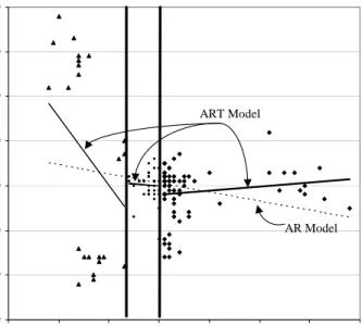
series data (one ofthe 2,494 data sets described in Section 4) shown in Figure 2.

Here,thedataisshownasascatterplotofy

t

versusy

t 1

. Alsoshownonthisplot

are AR(1) andART(1) models learnedfrom this data. Wecansee that theART

-1500

-1000

-500

0

500

1000

1500

2000

-1500

-1000

-500

0

500

1000

1500

2000

ART Model

AR Model

C

u

rrent

Value

(Y

t

)

Previous Value (Y

_t-1

)

Figure2. Scatterplotof time-seriesdataandAR(1) andART(1)models.

does theAR model. ART models that include additionalpredictor variables can

providefurther benetsoverAR models, although itis diÆcultto illustratethese

benetswithasimple(two-dimensional)gure.

In Section 3, we shall discuss computationally eÆcient methods for

learn-ing ART(p) models from data. In Section 5, we show that the resulting models

yieldaccurateforecasts. Finally,becauseARTmodelsaresimplepiece-wiselinear

predictors, they are easy to interpret. These three properties makeART models

particularlysuitablefordatamining.

2.2 Other Non-linear Autoregressive Models

There are a wide variety of alternative non-linear modeling techniques that have

been applied to time-series analysis (see, e.g.,[8]). In fact,as we describebelow,

onecantransformthetime-seriesproblemintoaregressionproblemandapplyany

non-linearornon-parametricregressiontechnique.

ThemostcloselyrelatedfamiliesofmodelstoARTmodelsaretheself-exciting

threshold autoregressive models (SETAR) of Tong [16] and the adaptive smooth

threshold regressivemodels (ASTAR) of Lewis, Ray, and Stevens [14]. Both the

SETARandASTAR models,aswellasARTmodels, arepiece-wiselinearmodels.

Describedintermsofadecisiontreerepresentation,theSETARmodelsarelimited

to a single split variable. Because of this limitation we do not further consider

ofthewell-knownmultiple adaptiveregressionsplines(MARS)system[7]to

time-series data. ARTmodels areprimarily distinguishedfrom the ASTAR models in

twoways(1)theerrorestimatesforanARTmodel candierbetweeneachofthe

pieces of the piece-wise linear model, and (2) the ART models allow there to be

discontinuitiesbetweenthepiece-wiselinearmodels.

Another common technique for non-linear time-series analysis is the use of

neuralnetworks. Although thesemodelscanlead toreasonablepredictive

perfor-mance, theyare diÆcult to interpret and can be expensiveto learn. Thus, these

modelsarelessusefulfordataminingandwedonotconsider themfurtherin this

paper.

3 Learning and Forecasting with ART Models

Inthissection,weshowhowtolearnthestructureandparametersofARTmodels

from observedtime-series data and how to usean ARTmodelfor forecasting. In

Section3.1,wedescribeageneralBayesianapproachforlearningmodelsfromdata.

InSection3.2,wedescribehowto calculateaBayesianscoreforchoosinganART

modelstructure. InSection3.3,wedescribesearchtechniques thatcanbeused in

conjunctionwithourBayesianscoretoidentify goodmodelsfromdata. Finally,in

Section3.4,wedescribehowtoforecastwithanARTmodel.

3.1 Learning Framework

LetusconsiderageneralBayesianapproachtolearning. Inthisapproach,wehavea

collectionofalternativemodelstructuress

1 ;:::;s

S

havingunknownmodel

param-eters s 1 ;:::; s S

,respectively,andweexpressouruncertaintyaboutthestructure

andparametersbyplacingprobabilitydistributions onthem: p(s)andp(

s js)|we

omitthestructuresubscriptsfromwhenclearfromcontext. WethenuseBayes'

ruleinconjunctionwiththedatadtoinferposteriordistributions overthese

quan-tities: p(sjd)and p(jd;s). Inthemostgeneralcase,wethenmakepredictionsby

averagingoverthese distributions. Thisapproach, however,is typically

computa-tionally intractable. Consequently,weuse aBayesian-modelselectionapproach in

whichwechoosethe structures that hasthe highestposteriorprobability p(sjd),

andmakepredictionsaccordingtop(jd;s)forthat s.

The key quantity in this Bayesian approach is the posterior probability of

model structure p(sjd). By Bayes' rule, this posterior probability is given by

p(sjd) = p(s)p(djs)=p(d). Because p(d) is a constant we can use the

prod-uct p(s)p(djs) to choose the best model. We shall refer to this product as the

Bayesian score for the model. The rst term in this score is simply the

struc-tureprior. Thesecond termp(djs)iscalledthemarginal likelihoodandisequalto

R

p(dj;s) p(js) d, the likelihood of the data p(dj;s) averagedoverthe

uncer-taintyin.

It is interesting to note that, when used for model selection, the marginal

likelihoodbalancesthetofthemodelstructuretodatawiththecomplexityofthe

N islarge,themarginallikelihoodcanbeapproximatedby p(dj ^ s ;s) jj 2 logN where ^ s

isthemaximum-likelihoodestimatorofthedata(see,e.g.,[10])formodel

s. Therstquantityinthisexpressionrepresentsthedegreetowhichthemodelts

thedata,which increasesasthemodelcomplexityincreases. Thesecondquantity,

incontrast,penalizesmodelcomplexity.

Now,letusturntotheapplicationoftheBayesianapproachtolearninga

sta-tionary,p-orderMarkovtime-seriesmodel. AccordingtoEquation1,thelikelihood

ofthedatais p(y p+1 ;:::;y T jy 1 ;:::;y p ;;s)= T Y t=p+1 f(y t jy t p ;:::;y t 1 ;;s) (4)

In this equation, we have included s to emphasize that we are learning model

parameters and model structure. Note that, in writing this likelihood, we have

omittedtherst pobservations, becauseap-order Markovmodel cannotpredict

theseobservations.

Giventhislikelihood,wecanproceedwithlearningasdescribedintheprevious

paragraphs, placing priors on model structures and model parameters and using

Bayes' rule. In the following section, we discuss this approach in detail for the

ARTmodel. Intheremainderofthissection,wedescribeastandard\windowing"

approachin theliteraturethat reducesourproblem tothe problemoflearningan

ordinarylinearregressionmodels(e.g.,[8]).

At the heart of the windowing approach is a transformation of the single

sequence y = (y 1 ;:::;y T ) to a set of cases x 1 ;:::;x T p . The transformation is givenby x i =(x i 1 ;:::;x i p+1 ), for 1<i <T p,where x i j =y i+j 1 . Wecall this

transformeddatasetthelengthptransformationofthetime-seriesdataset. Asan

example,consider thesequence y =(1;3;2;4). Then, thelength-2 transformation

is x 1 = (1;3);x 2 = (3;2);x 3

= (2;4), and the length-3 transformation is x 1

=

(1;2;3);x 2

=(2;3;4).

Giventhistransformation,wecanrewritethelikelihoodofthemodelin

Equa-tion4asfollows: p(y p+1 ;:::;y T jy 1 ;:::;y p ;;s)= T Y t=p+1 f(x t p+1 jx t 1 ;:::;x t p ;;s) (5)

This likelihood is precisely the likelihood for an ordinary regression model with

target variable X

p+1

and regressorvariables X

1 ;:::;X

p

. Thus, wecanlearn

sta-tionary,p-orderMarkovmodeltime-seriesusinganyordinaryregressiontechnique,

includingdecisiontrees.

Finally,wenotethat thisgeneralapproachofBayesianmodelselectionusing

p(sjd) to choose the model structure (including the order of the Markov process

modelshavingdierentvaluesofp,thenumberofproducttermsinthelikelihoodof

Equation5(or Equation4)willvary, makingcomparisonsdiÆcult. Oneapproach

to overcome this complication is to choose a small maximum value p 0

of p for

consideration, and includingonly those termsfor t p 0

in the product. Another

approach is to divide the marginal likelihood of a model by thenumber of cases

usedtocomputethemarginallikelihood. Thelatterapproach,whichweuseinour

experiments,isjustiedbytheprequentialinterpretationofthemarginallikelihood

asdescribedbyDawid[5].

3.2 The Bayesian Score for an ART Model

NowletusconsidertheBayesianscoreforanART(p)model. TofacilitateeÆcient

computation, it is desirableto havemodelscores that canbe computed in closed

form and factor according to the structure of the decision tree (e.g., [2]). It is

thisdesirethat leadsusto makethefollowingtwoassumptions. One,theapriori

likelihoodofamodelstructuresisgivenby

p(s)= jj

where0<1andjjisthenumberofmodelparameters. Inourexperiments,we

useaxedvalue=0:1,avaluewehavefoundtoworkwellformanyotherdomains.

Two, theparameters

1 ;:::;

L

|theparametersassociatedwith theleavesofthe

decisiontree|aremutually independent. Together,theseassumptionsimply

score(s)= L Y i=1 LeafScore(l i ) (6) where LeafScore(l i )= p+2 Z Y x t atl i f i (x t p+1 jx t 1 ;:::;x t p ; i ;s)p( i js)d i (7) wheref i

istheNormaldistributioncorrespondingtothelinearregressionatleafl

i ,

asdescribedinEquation3. LeafScore(l

i

)istheproductof(1)thepriorprobability

oftheleaf-componentofthestructure(therearep+2parametersateachleaf)and

(2)themarginallikelihoodofthedatathatfalls totheleaf.

The remaining ingredientfor the Bayesianscore is the parameter prior. In

thiswork,weusethetraditionalconjugatepriorforalinearregression. Namely,we

assumethat

i

hasanormal-gammaprior(e.g.,[1]). IntheAppendix,wederivethe

formulasforLeafScore(l

i

)giventhisprior. Wenotethatthisscorecanbecomputed

inclosedformandhasacomputationalcomplexityofO(p 3 +p 2 C i ),whereC i isthe

numberofcasesthatfall toleafl

i .

3.3 Searching for ART-Model Structure

Inthissection,wedescribetwoapproachesforlearningthestructureofARTmodels

Therstlearningmethodis forlearningthestructure foranART(p)model when

wearegiven p;the secondmethod isforlearningthestructureforanARTmodel

when weare not given p. Whenwedescribe ourresults in Section 5, we callthe

resultoftherstmethod anARTmodel for known pandtheresultof thesecond

methodanARTmodelfor unknownp. BecauseARmodelsareaspecialcaseofan

ARTmodelwecanalso learnAR models with known pand unknownp. Each of

thesefourmethodsis usedinourexperiments.

Ourmethod forlearninganART model withknown p|thatis, forlearning

thesplitvariablesandsplitvaluesforadecisiontreewhenthepossiblesplitvariables

are limitedto theprevious ptime periods and the leaves containa regressionon

p regressors|is as follows. We use a greedy search algorithm that employs the

operatorsplit-leaf. Theoperatorisappliedtoaleafofadecisiontreeandtakestwo

arguments: avariable to split onand the valueof thevariable. Forinstance, the

decisiontree in Figure 1was obtainedbythe application ofsplit-leaf(Y

i 1 ; 337)

to thesingle leafof an empty decisiontree (the root) followedby theapplication

ofsplit(Y

i 1

;0)to therightchildof thedecisiontreeresultingfromtherstsplit.

Whenapplyingthesplit-leafoperatortoleafl

i

,werestrictattentiontopotentially

splittingonsevenvaluesofeachpredictorvariable;thesevaluesaretheboundaries

of eight equiprobable contiguousregions of anormal distribution estimated from

therestricteddatasetattheleafforthepredictorvariable(see[3]forajustication

of the choice of eight regions). The initial decision tree is a decision tree with a

singleleaf, that is, nosplits. We growadecision treeby iterativelyapplying the

split-leafoperatortoeach leafforeachvariable,andchoosingthesplitthatresults

inthelargest(non-negative) increaseinmodelscore. Ifnosplit onanyleafyields

ahigherscore,thenthesearchisterminated.

Thegreedyprocedureiscomputationallytractable. Recallthatasingle

eval-uation of a split-leaf operator applied to leaf l

i

has computational complexity

O(p 3 +p 2 C i ), where C i

is the number of cases that fall to leaf l

i

. In addition,

foreach leaf,wesearch among ppotential split variablesand search among (e.g.)

k = 8 possible split points. Also, because the splits are binary, the number of

leafnodesthat areevaluatedforexpansionisalwayslessthantwicethenumberof

leavesintheresultingtree. Thus, becauseC

i

<T,theoveralllearningtimegrows

asO(kL(p 4

+p 3

T)),where L isthenumberofleaves. Aswith otherdecision-tree

learningalgorithms,thelearningtimeisafunctionofthesizeofthetree. Typically,

asoneincreasesthesizeofadataset,thesizeofthelearnedtreegrowsandthusthe

timetolearndoesnotnecessarilygrowlinearlyinthesizeofthedataset. Despite

thispotentialsuper-linearscaling,wendempiricallythatdecision-treealgorithms

scalealmost linearlyforlargedatasets.

WelearnanARTmodelwithunknownpbyrepeatedlyusingthemethodfor

learninganARTmodelwithknownp. Inparticular,welearnanART(i)modelfor

each0ip

max

,andchoosethemodelwiththehighestBayesianscore.

3.4 Forecasting with ART Models

Wenowconsider theproblem ofusing ART modelsto forecast. Givenasequence

observationsin thesequence. Wedistinguishbetweentwoimportanttypesof

fore-casting: (1)one-stepforecastingand(2)multi-stepforecasting. Inourevaluationof

predictiveaccuracy,weuseone-stepforecasting.

Inone-stepforecasting,we areinterestedinpredictingy

T+1

giveny

1 ;:::;y

T

areknown. Forthis situation,theposterior distributionforthevariable Y

T+1 isa

function ofasingleleafnode inthe tree. Inparticular, usingthe conjugatepriors

we have described, each leaf in the tree has a conditional t-distribution for this

variable. Inourexperiments,dueto limitationsin ourimplementation, wedonot

usetheappropriatet-distributiontocomputetheselog-likelihoods. Instead,weuse

thenormaldistributionf

i (y t jy t p ;:::;y t 1 ; i

)(describedinEquation3)evaluated

at the value of

i

that is most likely given the data|the maximum a posteriori

(MAP)value: ~ i =argmax Y x t atli f i (x t p+1 jx t 1 ;:::;x t p ; i ;s)p( i js) (8)

Adetailed expressionfor ~

i

isgivenintheAppendix.

Inmulti-step forecasting,weare interestedin predictingvaluesfor variables

atmultiplefuturetimesteps. Whenforecastingmorethanonestepintothefuture,

a simple lookup is not possible due to the non-linearities in the AR tree. For

example,wemayhavetheART modelfrom Figure 1,andwish topredict Y

4 ,Y 5 , and Y 6

when weknow thevalues for onlyY

1 andY

2

. The predictionfor Y

4 does

not correspond to a singleleaf becausewedo not know the valueof Y

3

. Insuch

situations,onecanapplyacomputationallyeÆcientMonteCarloapproachsuchas

forwardorlogicsampling[12]. Inthisapproach,onesamplesy

T+1 giveny 1 ;:::;y T , theny T+2 giveny 1 ;:::;y T+1

,andsoon,usingeithertheappropriatet-distribution

orMAP(normal)distribution. Thesesamplesarethenusedtoestimatequantities

of interest such as the expected values and variances for variables at future time

steps.

4 Evaluation

Inthis section, weprovide anempiricalevaluation ofourmethods and several

al-ternativemethods. Toevaluatethe methods, weuse the2,494 largesttime-series

data sets from the M3 competition available from the International Institute of

Forecasters(http://forecasting.cwru.edu/Data/m3comp/m3comp.html). Thetime

seriesvaryinlengthfrom23to126periodswithboththemedianandmeanlengths

larger than 60periods. The data sets are from avariety of sources including

in-dustrial production data, micro andmacro economic data, and nance data. We

eliminatedatasetssmallerthan23periodstoallowforafaircomparisonwithone

ofthe methods(MARS) which (quitereasonably)couldnotbeapplied tosmaller

datasets.

Foreach ofthe data sets, wecreate nine data sets using thelength p

trans-formation (described in Section 3.1) with p varying from zero to eight. Each of

these transformeddata setsis centeredand standardizedbeforemodeling;that is,

Wedivide each dataset intoatrainingset, usedasinputtothe learningmethod,

andaholdoutset,usedtoevaluatethemodels. Theholdoutsetcontainsthecases

correspondingtothelastveobservationsinthesequence.

Weevaluatethequalityofalearnedmodelbycomputingthesequential

pre-dictivescorefortheholdoutdatasetcorrespondingtothetrainingdatafromwhich

themodel waslearned. The sequentialpredictivescorefor amodelis theaverage

log-likelihoodofthecasesintheholdoutset,wherethelog-likelihoodofacaseisthe

logprobabilitythat themodel assignsto theobservedvalueofthetarget variable

given the observed predictor values. This log-likelihood computation is simply a

one-step forecast. Finally, to evaluate thequality of alearningmethod, we

com-pute the average of the sequential predictivescores for each of the 2,494 learned

modelsproducedbythelearningmethod. Notethattheuseofthelog-likelihoodto

measure performance simultaneouslyevaluates both the accuracy of the estimate

andtheaccuracyoftheuncertaintyof theestimate.

Inourexperiments,wecomparethefollowinglearningmethods: the Salford

SystemsimplementationofFriedman'smethodforlearningMARS(ASTAR)

mod-els[7],animplementationof asimpleregression-treelearningalgorithm described

byChickering et al. [3], and themethods described in Section 3 forlearningAR

andARTmodels.

Weapplythelearningmethodsto transformeddatasets usingnine dierent

transformationlengths(0p8). Thus, foreach dataset, welearnnine MARS

models,nineregression-treemodels,nineARmodelswithknownp,andnineART

models with known p. We additionally learn eight AR and ART models with

unknownp(0<p

max 8).

5 Results

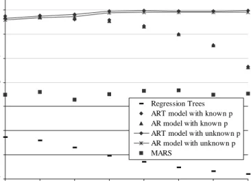
Theresultsofourexperimentsaresummarizedin Figure3. Inthisgure,weplot

the average sequential predictive scores for the models learned by the candidate

learningmethods. Thep th

point for alearning method is the average sequential

predictivescoreforthe2,494modelslearnedbythatmethod whenwerestrictthe

maximumdependencyto lengthp. Note thattheresultsoflearningAR andART

models with known p will havea dependency length of exactlyp. Weemphasize

the results for AR models with known p and for ART models with known p by

connecting the points with a curve. We do not plot the results of the learning

methods applied to the length-zerodata transformations. The result of using an

ARmodelonthistransformeddataobtainsanaveragesequentialpredictivescore

of-9.03. Theresultsoftheothermodelsarenearly identical.

Thepoorestperformingmodelsarethesimpleregressiontrees. Thefactthat

ARTmodels performsignicantlybetterindicates that allowingnon-triviallinear

regression at the leaves of the decision tree is important when modeling a time

series.

TheMARS method performs signicantlybetter thanthe simple regression

treebutworsethantheothermethods. Onepossibleexplanationofthisdierenceis

-8.7

-8.5

-8.3

-8.1

-7.9

-7.7

-7.5

-7.3

1

2

3

4

5

6

7

8

Maximum Dependency Length

A

v

er

ag

e

P

re

d

ict

iv

e

S

co

re

Regression Trees

ART model with known p

AR model with known p

ART model with unknown p

AR model with unknown p

MARS

Figure3. Comparisonofmethods.

necessarily depend on all of the p previous predictor variables. In contrast, the

forecastsmadebyMARSmodelsofteneliminatedsomeofthesepredictorvariables.

Infact, in manyofthe data sets, thebackwardstep-wise elimination stage ofthe

MARS method (see Friedman, 1991) eliminated all dependence on the predictor

variables. Thus, AR(p) and ART(p) place moreemphasis on recent timeperiods

forprediction,whichmayhaveledtobetterpredictions. Perhapsonecouldimprove

theperformanceoftheMARSsystembybiasingthesearchand selectionof knots

towardsrecenttimeperiods.

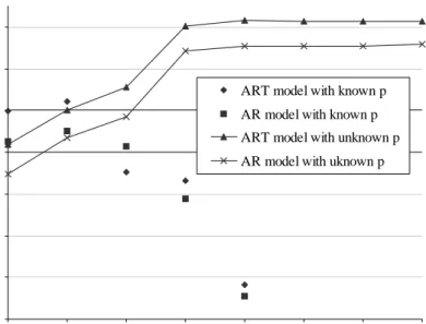
In Figure 4, we concentrate on the performance of the AR and ART

mod-elsthat are learnedwith known andunknown p. The fact that both theAR and

ARTcurveswithknownp(correspondingtomodelselectionforp)increaseroughly

monotonicallyis evidence thatour approach tomodelselection isworking.

Addi-tionally, thecomparison of therespective\known p"and \unknown p" pointsfor

the AR andART models indicate the benetsof model selection. Namely, aswe

includemoremodelsweareabletoimproveourpredictivescore|choosingmodels

that providegoodt withwithoutovertting. Nonetheless, thisbenettaperso

as p

max

increases. Note that thereis alargeincreasein performanceforbothAR

andARTmodelswhenallowingdependenciesatalagoffour. Webelievethisjump

is due, in part, to the fact that roughly onefourth of ourdata sets are quarterly

(e.g. quarterlysalesresultsforacompany).

InFigure 4, thecurve forART model with unknownpdominates thecurve

for AR model with unknown p indicating that the additional exibility of ART

modelsto modelnon-lineardependenciesleadsto bettergeneralization. Whilethe

dierencesinpredictiveaccuracyforvariousp

max

arenotaslargeasthedierences

-7.45

-7.43

-7.41

-7.39

-7.37

-7.35

-7.33

-7.31

1

2

3

4

5

6

7

8

Maximum Dependency Length

A

v

er

age

P

re

di

ct

iv

e

S

co

re

ART model with known p

AR model with known p

ART model with unknown p

AR model with uknown p

Figure4.EectivenessofmodelselectionandcomparisonofARandART

models.

Thep-valuesforallvaluesofp

max

arelessthan0:001forthesigntestandsmaller

fortheWilcoxonsigned-ranktest.

Recallthat anART modelwith nosplitsis anARmodel; thus,thelearning

procedure forART models canreturnanAR model. Wenote that in only5% of

thedatasetsdidtheresultingARTmodelhaveatleastonesplit. Thefact thata

largefractionofARTmodelshavenosplitsisdue,inpart,tothefactthatthedata

sets arefairlyshort time series. This explanationis supported bytheobservation

thatthenumberofsplitschosenbyourmethodiscorrelatedwiththelengthofthe

timeseries. WesuspectthatthebenetsofARTmodelswithrespecttoARmodels

willincreasewhenappliedtolongertimeseries.

6 Summary and Future Work

Ourexperimental resultsshowthat ARTmodelsare auseful familyofmodelsfor

time-seriesanalysisandourBayesianapproachtolearningARTmodelscanidentify

predictively accurate models. In addition, coupled with our method for model

selection,ARTmodelsprovideatractablefamilyofmodelsformodelingtime-series

datathatimproveonthestandardARmodels. Also,ARTmodelsprovideasimple

interpretablealternativetoothernon-lineartechniquessuchasneuralnetworks. Of

course,thereismoreworktobedoneinunderstandingthebenetsofARTmodels

andinimprovingtheirperformanceontime-seriespredictiontasks.

models. BecauseARtreesaresimplydecisiontreesapplied totime-seriesanalysis,

anysystemthatlearnsdecisiontreeswithlinearregressionsattheleavescanbeused

to build anAR tree. Several such systemsexist including theRETIS system[13]

andtheM5system[15]. ThesetwosystemsdierinthattheRETISsystemusesall

ofthefeaturesinthelinearregressionandusesthelinearregressiontoevaluatethe

modelduringthegreedyconstructionofthedecisiontree,whereastheM5addsthe

linearregressionwhilepruningthedecisiontreeandcanpotentiallyprunefeatures

fromthelinear-regression. Anotherapproachforlearningdecisiontreeswithlinear

regressionsattheleavesisdescribedbyChipman,George,andMcCulloch[4]. Their

BayesianapproachusesaMarkovChainMonteCarlotechniquetoexplorethespace

ofalternativemodels. Itwouldbeusefultocompareourapproachwithalternative

methods(includingalternativemethodsforlearningdecisiontrees)forthepurpose

oftime-seriesanalysisandotherregressionproblems.

In this paper, we have focused on ART(p) models with the following two

restrictions: (1)thesplit variablesarechosenfromamongtheppreviousvariables

and(2)theleavescontainAR(p)models. OurmethodforlearningART(p)models

canbeadaptedtoremovetheserestrictions. First,wecanexpandthesetofpossible

covariatesforoursplit-leafoperatorto includeadditionalcovariates(evendiscrete

covariates,e.g.,monthinadailytimeseries). Second,wecanincludeasearchover

subsetsofregressors. Itwould usefultoinvestigatethebenetsofthese andother

methodsforrelaxingtherestrictions.

ART models and our method for learningthem can also beadapted to the

analysisofmultivariatetimeseries(e.g. salesresultsfrommorethanonecompany).

Multivariatetimeseries canbehandled in twoways: (1) learndecisiontreeswith

multivariateregressionsin theleaves,or(2)learnaseparate ARTmodel foreach

timeseriesallowingforregressorsfromalltimeseries. Wesuspectthatthesecond

approachwouldbebetter,butfurther evaluation isneeded.

Wenotethat,bylearningasingletreewithMAPparametervalues,our

ART-model forecasting procedure ignores both structure and parameter uncertainty.

Structureuncertainty(includinguncertaintyaboutsplit points) canbetaken into

accountusingfullorpartialmodelaveraging(e.g.,[1]),butthecomputationalcost

isoftenprohibitive. Aswehavediscussed,parameteruncertaintycanbetakeninto

accountin acomputationally tractable mannerusing t-distributions. It would be

usefulto understandtherelativeimportance ofhandlingthese twocomponentsof

uncertainty.

Finally,oneimportantaspectofmodelingtimeseriesishandlingseasonalityin

data. SeasonalitycanbehandledusingARTmodelsbyexplicitlyallowingor

includ-ingrelevantregressorvariablesinthelinearregressionsattheleaves. Alternatively

onecanusestandardtechniquestode-seasonthedatapriorto theconstructionof

anARTmodel. Furtherexperimentationisneededtocharacterizetheperformance

Bibliography

[1] J.BernardoandA.Smith.BayesianTheory. JohnWileyandSons,NewYork,1994.

[2] D. Chickering, D. Heckerman, and C.Meek. ABayesianapproach to learning Bayesian

networkswithlocal structure. InProceedings of Thirteenth ConferenceonUncertainty in

ArticialIntelligence,Providence,RI.MorganKaufmann,August1997.

[3] D.Chickering,C.Meek,andR.Rounthwaite.EÆcientdeterminationofdynamicsplitpoints

inadecisiontree.InProceedingsofthe2001IEEEInternationalConferenceonDataMining,

pages91{98,SanJose,CA,November2001.IEEEComputerSociety.

[4] H.Chipman,E.George,and R.McCulloch. Bayesiantreedmodels,to appear inMachine

Learning. Technical Report http://bevo2.bus.utexas.edu/GeorgeE/Research

papers/treed-models.pdf,UniversityofWaterloo,2001.

[5] P.Dawid. Statisticaltheory. Theprequential approach (withdiscussion). Journal of the

RoyalStatisticalSocietyA,147:178{292,1984.

[6] M.DeGroot. OptimalStatisticalDecisions.McGraw-Hill,NewYork,1970.

[7] J.Friedman. Multivariateadaptiveregressionsplines.AnnalsofStatistics,19,1991.

[8] N.GershenfeldandA.Weigend. Thefutureoftimeseries: learningandunderstanding. In

Timeseriesprediction,pages1{70.AddisonWesley,NewYork,1994.

[9] J.Hamilton.TimeSeriesAnalysis.PrincetonUniversityPress,Princeton,NewJersey,1994.

[10] D.Haughton. Onthe choiceofa modelto tdata fromanexponentialfamily. Annals of

Statistics,16:342{355,1988.

[11] D. Heckerman and D.Geiger. LearningBayesian networks: Aunication fordicrete and

Gaussiandomains.InProceedingsofEleventhConferenceonUncertaintyinArticial

Intel-ligence,Montreal,QU,pages274{284.MorganKaufmann,August1995. SeealsoTechnical

ReportTR-95-16,MicrosoftResearch,Redmond,WA,February1995.

[12] M.Henrion.PropagationofuncertaintybyprobabilisticlogicsamplinginBayes'networks.In

ProceedingsoftheSecondWorkshoponUncertaintyinArticial Intelligence,Philadelphia,

PA.AssociationforUncertaintyinArticialIntelligence,MountainView,CA,August1986.

Also inKanal, L.and Lemmer,J., editors, Uncertainty in Articial Intelligence 2, pages

149{164.North-Holland,NewYork,1988.

[13] A.Karalic.Employinglinearregressioninregressiontreeleaves. InProceedingsofECAI-92,

pages440{441.JohnWiley&Sons,1992.

[14] P.Lewis, B. Ray, and J. Stevens. Modeling time seriesby using mars. In Time series

prediction,pages297{318.AddisonWesley,NewYork,1994.

[15] J.R.Quinlan.Learningwithcontinuousclasses.InProceedingsofofthe5thAutralianJoint

ConferenceonArticialIntelligence,pages343{348.WorldScientic,1992.

[16] H.Tong. ThresholdmodelsinNonlinearTimeSeriesAnalysis. Springer-Verlag,NewYork,

Appendix

We derive formulas for LeafScore(l

i

) given by Equation 7, and for ~

i

, the MAP

parametersforthelinearregressionatleafl

i

givenbyEquation8.

HeckermanandGeiger[11]|hereinHG|makethefollowingassumptionsfora

setofobservationsd=(x 1 ;:::;x N )whereeachx t =(x t 1 ;:::;x t p+1 )isanobservation overvariablesX =(X 1 ;:::;X p+1

): (1)thelikelihoodofthedataforagivenmodel

structuresis Q N i=t p(x t 1 ;:::;x t p+1

j;W;s)whereeachtermisamultivariate-Normal

distributionwithunknownmeanvectorandprecisionmatrixW,(2)p(Wjs)isa

Wishartdistribution,and(3)p(jW;s)isamultivariate-normaldistribution. Under

theseassumptions,itfollowsthattherelationshipbetweenX

p+1 andX 1 ;:::;X p is

thelinearregression:

p(x t p+1 jx t 1 ;:::;x t p ;;s)=N(m+ p X j=1 b j x p ; 2 ); t=1;:::;N (9) where, m= p+1 p X i=1 b i i ; b j = p X i=1 (W 1 ) p+1;i (((W 1 ) pp ) 1 ) ij ; 2 =1=W p+1;p+1 : (10)

InEquation10,weusevector-matrixnotationinwhichv

i denotesthei th elementof vectorv,M ij

denotestheelementin thei th

rowandj th

columnofmatrixM,and

M pp

denotestheupperppsub-matrixofM. HG'sassumptionsalsoimplythat

=(m;b 1 ;:::;b p ; 2

) hasa normal-gamma distribution. Thus, when we identify

the casesin d with those that fall to leaf l

i

and identify in Equation9 with

i

in themainbodyofthetext,wendthatHG'sassumptions implytheconditions

leading to the expressions for LeafScore(l

i ) in Equation 7 and ~ i in Equation 8.

Thus,weusetheHGframeworktoderivethese quantities.

Followingtheirapproach,letp(jW;s)beamultivariate-normaldistribution

with mean

0

and precision matrix

W ( > 0), and p(Wjs) be a Wishart distributionwith W degreesoffreedom ( W

>p) andpositive-denite precision

matrixW

0

. Then,theMAPparametervalues|thosethatmaximizetheprobability

ofdgivenands|aregivenby

~ = 0 +N N +N and ~ W 1 = 1 W +N (p+1) W N where W N =W 0 +S N + N +N ( 0 N )( 0 N ) 0 (11)

Intheseandsubsequentequations,weusevectorv todenoteacolumnvectorand

v 0

todenotethetransposeofv(arowvector). Theterms

N andS

N

arethesample

meanandscattermatrix,respectively,givenby

N = 1 N N X t=1 x t and S N = N X t=1 (x t N )(x t N ) 0 (12)

WeobtaintheMAPvaluesfor=(m;b

1 ;:::;b

p

;)bytransformingthese

expres-sionsfor~and ~

W 1

accordingtothemappingin Equation10.

GivenHG'sassumptions, italsofollowsthat themarginallikelihoodis given

by p(djs)= (p+1)N =2 +N (p+1)=2 c(p+1; W +N) c(p+1; W ) jW 0 j W 2 jW N j W +N 2 (13) where c(l;)= l Y i=1 +1 i 2 : (14) In addition, (X 1 ;:::;X p

) has a (p-dimensional) multivariate-normal distribution

withunknownmeanandprecision,whichweshalldenote andW ,respectively.

Furthermore, p( jW ;s) has a multivariate-normal distribution with mean

0

(the rst p entries of ) and precision matrix

W , and p(W js) is a Wishart

distributionwith

W

1degrees of freedom and precisionmatrixW

0 such that (W 0 ) 1

is equalto theupper ppsub-matrix of (W

0 )

1

. Thus, ifweletd be

the data d restricted to the variables (X

1 ;:::;X

p

), then the marginal likelihood

p(d js)isgivenbythep-dimensionalversionofEquation13,with

0 ,W 0 ,and W , replacedby 0 ,W 0 ,and W

1,respectively. Finally,the(conditional)marginal

likelihoodisgivenby Z N Y t=1 p(x t p+1 jx t 1 ;:::;x t p ;;s)p(js)d i = p(djs) p(d js) : (15)

Substituting the expression for p(djs) given by Equation 13 and the analogous

expression for p(d js) into Equation 15, we obtain a formula for the

marginal-likelihoodcomponentofLeafScore(l

i ).

Inourexperiments,weuse

0 =0,W

0

=I (theidentitymatrix),

=1,and

W

=p+2appliedtodatathathasbeenstandardizedtohaveameanofzeroand