Open-cluster density profiles derived using a kernel estimator
Anton F. Seleznev
‹Astronomical Observatory, Ural Federal University, Mira str. 19, Ekaterinburg 620002, Russia
Accepted 2015 December 6. Received 2015 December 2; in original form 2015 June 10
A B S T R A C T
Surface and spatial radial density profiles in open clusters are derived using a kernel estimator method. Formulae are obtained for the contribution of every star into the spatial density profile. The evaluation of spatial density profiles is tested against open-cluster models fromN-body experiments withN=500. Surface density profiles are derived for seven open clusters (NGC 1502, 1960, 2287, 2516, 2682, 6819 and 6939) using Two-Micron All-Sky Survey data and for different limiting magnitudes. The selection of an optimal kernel half-width is discussed. It is shown that open-cluster radius estimates hardly depend on the kernel half-width. Hints of stellar mass segregation and structural features indicating cluster non-stationarity in the regular force field are found. A comparison with other investigations shows that the data on open-cluster sizes are often underestimated. The existence of an extended corona around the open cluster NGC 6939 was confirmed. A combined function composed of the King density profile for the cluster core and the uniform sphere for the cluster corona is shown to be a better approximation of the surface radial density profile.The King function alone does not reproduce surface density profiles of sample clusters properly. The number of stars, the cluster masses and the tidal radii in the Galactic gravitational field for the sample clusters are estimated. It is shown that NGC 6819 and 6939 are extended beyond their tidal surfaces.
Key words: open clusters and associations: general.
1 I N T R O D U C T I O N
Surface density profiles are traditional tools in investigations of the structure of stellar clusters. Surface density profiles have been used for cluster size determination, for example, by Sung, Sana & Bessell (2013), Santos-Silva & Gregorio-Hetem (2012) and Camargo, Bon-atto & Bica (2012). It should be noted that usually surface density profiles are plotted as histograms of star counts, and the stochastic-ity of histograms has prevented a reliable determination of cluster size. Methods have been presented to reduce both stochasticity and asymmetries. Kholopov and Artyukhina have performed star counts in a series of overlapping rings of different widths and in overlapping sectors (see, e.g. Artyukhina & Kholopov1962; Kholopov1963). Djorgovski (1988) proposed an averaging of star counts across sev-eral angular bins. Apart from stochasticity, the limited field of view is often the reason for the unreliable determination of cluster size.
Cluster density profiles can be compared with different dynamic models in order to reveal the results of different dynamic processes. For example, gravothermal catastrophe in globular clusters becomes apparent by means of post-collapse density profiles (Sosin & King 1995,1997; Miocchi et al.2013). Density profiles in the outer cluster parts reveal cluster disruption processes in the outer tidal field (e.g. Carraro, Zinn & Moni Bidin2007; K¨upper et al.2010b;
E-mail:[email protected]
Bello et al. 2012). The presence of mass segregation shows an efficiency of stellar encounters or – in the case of extremely young clusters – preferential birth places of stars with different masses or special features in the cluster formation process (e.g. Vesperini, McMillan & Portegies Zwart2009; Gennaro et al.2011; Goldman et al.2013; Pang et al.2013). Irregularities in the density profiles indicate the non-stationarity of a cluster in the regular field (Danilov & Putkov2012).
The extended sparse outer regions of open star clusters (i.e. cluster coronae) are of special interest. Danilov, Putkov & Seleznev (2014) have presented a modern review of arguments in favour of the existence of cluster coronae. The cluster coronae can extend over the open-cluster tidal surface. Stars leave the cluster through the tidal surface in the vicinity of Lagrange points (see, e.g. K¨upper, Macleod & Heggie2008; K¨upper et al.2010a). Some of these stars go fast at large distances from the cluster and form the cluster tidal tails. Others, before moving to tidal tails, can live in the close cluster vicinity (up to distances of four tidal radii of the cluster in the Galactic gravitational field) for a relatively long time, comparable with the mean lifetime of the cluster (Danilov et al.2014). This is the cluster corona. The formation of coronae in open clusters and in their numerical models can be explained by the formation of unstable periodic orbits and the large number of retrograde unclosed trajectories in the vicinity of such orbits (Danilov et al.2014).
The detection of the open-cluster coronae is difficult because of the low stellar density in the coronae, and because of the fluctuations
of the stellar density of the background. The parameters of the open-cluster coronae can be determined more firmly and reliably after identifying probable cluster members, taking into account the data on the stellar proper motions (see, e.g. Artyukhina1970). Danilov, Matkin & Pylskaya (1985) proposed the method of star counts (referred to hereafter as the DMP method), based on the use of the function N(r), the number of stars in the circle of radiusr. This method was used by Danilov & Seleznev (1994) to study the structure of 103 open star clusters. The method involves the comparison of the cluster field with several fields of the cluster neighbourhood. This requires the study of a very large region around the cluster (with a radius of up to six cluster radii). The use of this method is restricted by large-scale fluctuations of the stellar background density in the cluster vicinity. The goal of the present paper is to use the surface density functionF(r), derived with the kernel estimator, in order to search for the coronae of the open clusters.
The surface densityF(r) is the number of stars per unit area of the celestial sphere,
dN=2πrF(r)dr, N=2π
R
0
F(r)rdr, (1) whereris the current distance from the cluster centre andRis the radius of the circle (sphere) around the cluster centre. The spatial densityf(r) is the number of stars per unit volume of the coordinate space,
dN=4πr2f(r)dr, N=4π
R
0
f(r)r2dr. (2)
The use of radial density profiles assumes the hypothesis of a spherical symmetry. Both the surface and spatial stellar densities are connected with the corresponding probability densities: ϕ(r)= 2πr N F(r) , R 0 ϕ(r) dr=1; (3) ψ(r)= 4πr 2 N f(r), R 0 ψ(r) dr=1. (4) Consequently, methods of probability density evaluation can be used to obtain the surface and spatial densities. Such methods have been considered by Silverman (1986). The kernel estimator stands out among these because of its intuitive clarity and relatively simple realization. The essence of the kernel estimator method is the fol-lowing. Every data point in the sample is replaced by some function (kernel) normalized by 1. The result of the probability density is the sum of all kernels divided by the number of sample pointsN. Estimates of the surface or spatial density are obtained as the sum of kernels, not divided byN. It is very important that the density es-timate inherits the properties of the kernel function (e.g. continuity and differentiability in the case of kernels used in this paper).
The kernel estimator was used in previous research to estimate the luminosity function and to derive and analyse surface density maps in star clusters (Seleznev1998; Seleznev et al. 2000; Prisinzano et al.2001; Pancino et al.2003; Kirsanova et al.2008; Seleznev et al.2010; Carraro & Seleznev2012).
Merritt & Tremblay (1994) used the kernel estimator and the maximum penalized likelihood estimator to estimate density pro-files. They showed that the one-dimensional kernel estimator was not appropriate for a surface density profile construction, and a two-dimensional method was needed. Merritt & Tremblay (1994) obtained formulae for a kernel function for the case of the sur-face radial density profile and obtained estimates for spatial
den-sity solving an Abel equation. They investigated the efficiency of both methods for three important distributions (Plummer, de Vau-couleurs, Michie–King) and showed that the use of an ‘optimal’ kernel half-width, determined with the minimization of the inte-grated mean-square error, led to an unsatisfactory result. Merritt & Tremblay (1994) proposed an empirical selection of kernel half-widths (i.e. obtaining a series of profile estimates and selecting the best version); that is, ‘simply looking at plots produced using sev-eral different values of the smoothing parameter, and accepting the one that is as smooth as possible without being obviously biased – that is, the smoothest curve that closely follows the mean trend de-fined by curves computed with much smaller smoothing parameter.’ They used both kernel and maximum penalized likelihood methods to derive surface density profiles for the Coma cluster of galaxies and for the M15 globular cluster.
In the present work, a kernel estimator is used to construct sur-face radial density profiles for seven open clusters, and to construct spatial radial density profiles for the numerical models of the open-cluster coronae obtained byN-body experiments withN=500. The paper is organized as follows. Section 2 is devoted to the develop-ment of formulae for surface and spatial density profiles. The spatial density profiles of the coronae of theN-body open-cluster models are derived in Section 3. Section 4 contains a description of the derivation of the surface density radial profiles for seven open clus-ters, and a discussion of the profiles. The estimation of the cluster sizes is discussed in Section 5, and the results of the present paper are compared with the data from the literature. Section 6 describes an approximation of the cluster radial surface density profiles using the King profile, with and without considering the contribution from the cluster corona. The cluster mass and the tidal radii estimates are obtained in Section 7. Conclusions are given in Section 8.
2 K E R N E L E S T I M AT O R F O R S U R FAC E A N D S PAT I A L R A D I A L D E N S I T Y P R O F I L E S
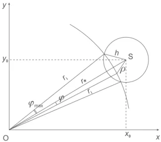
To understand the derivation of the formulae better, let us begin with the case of the surface density profile. Consider the plane (x,y) tangent to the celestial sphere at the point of cluster centre O (see Fig.1). Point S is the projection of a star to the tangent plane, the circle with centre S is the projection of the kernel with half-widthhandr∗is the distance of the star from the cluster centre
in the projection. The contribution of this star to the surface density profile estimate at the distancerifrom the cluster centre is evaluated. The kernelK2(Silverman1986, see equation 4.5) is used for the calculation of the surface density. This kernel corresponds to the contribution to the surface density as
F = ⎧ ⎨ ⎩ 3 πh2 1−ρ 2 h2 2 with ρ < h, 0 with ρ≥h. (5)
This kernel function (often called the ‘quartic’ kernel) has an advantage in the computational aspect. Namely, this function has high smoothness properties in contrast to the Epanechnikov ker-nel, which allow us to use a reasonably coarse grid for contouring without introducing appreciable errors (Silverman1986). This is important especially when plotting two-dimensional maps of the surface density. Another kernel – the Gaussian kernel – is excel-lent in differentiability, but it requires a much greater amount of computations (Merritt & Tremblay1994).
In order to obtain the contribution of star S to the surface density profile at the distancerifrom the cluster centre, we need to integrate this function byϕover the arc of the circle with radiusrifrom−ϕmax
Figure 1. The plane (x,y) is the tangent plane to the celestial sphere at the point of the cluster centre O. Point S is the projection of a star to the tangent plane, the circle with centre S is the projection of the kernel with half-width handr∗is the distance of the star from the cluster centre in the projection. The case|r∗−ri|< h.
Figure 2. Same as in Fig.1, but for the caseri< h−r∗. toϕmax(which is the case when|r∗−ri|< h; see Fig.1). The result
is F(ri)= 3 π2h2 1−r 2 i +r∗2 h2 2 ϕmax+6r 2 ir∗2 π2h6ϕmax +12rir∗ π2h4 1−r 2 i +r 2 ∗ h2 sinϕmax+3r 2 ir 2 ∗ π2h6sin 2ϕmax, (6) where ϕmax=cos−1 r2 i +r∗2−h2 2rir∗ .
Another situation is possible: when the circle of radiusri lies inside the circle of the kernel (ri< h−r∗; see Fig.2). In this case,
we need to integrate equation (5) byϕfrom 0 to 2π. The result is F(ri)= 3 πh2 1− r 2 i +r 2 ∗ h2 2 +6ri2r 2 ∗ πh6 . (7)
Figure 3. Star S at distance r∗ from cluster centre O and the three-dimensional kernel with half-widthh: the case of|r∗−ri|< h.
It is easy to show that equations (6) and (7) coincide with equation (28b) from Merritt & Tremblay (1994).
The same approach is used for the determination of the contribu-tion of the star into the spatial density when the spatial coordinates (x,y,z) of the star are known. The multivariate Epanechnikov ker-nel (Silverman1986, see equation 4.4) for three dimensions is used for the case of spatial density. It corresponds to the contribution to spatial density as f = ⎧ ⎪ ⎨ ⎪ ⎩ 15 8πh3 1−ρ 2 h2 with ρ < h, 0 with ρ≥h. (8)
The Epanechnikov kernel in the case of three dimensions was also selected because of computational considerations. It gives simpler equations for the density profile in contrast to the quartic kernel, and requires fewer computations in contrast to the Gaussian kernel. In addition, there is very little difference between the Epanechnikov, quartic and Gaussian kernels in many aspects (Silverman 1986; Merritt & Tremblay1994).
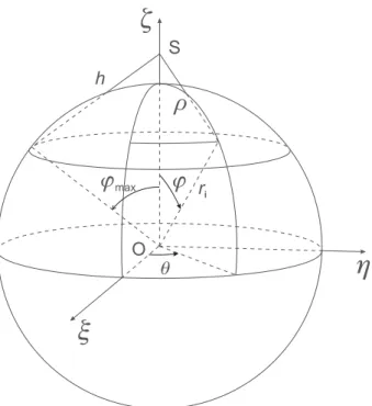
Fig.3shows star S at distancer∗from cluster centre O and the
three-dimensional kernel with the half-widthh. The contribution of this star to the spatial density profile at distancerifrom the cluster centre is calculated. Fig.4shows the sphere with radiusriaround the cluster centre. The coordinate system in Fig.4was transformed into (ξ,η,ζ) with axisζin the direction from the cluster centre to star S. In order to obtain the required contribution, it is necessary to integrate the function in equation (8) over the segment of this sphere byθfrom 0 to 2πand byϕfrom 0 toϕmaxin the case shown in Fig.4(|r∗−ri|< h) or from 0 toπin the case when the sphere
of radiusrilies inside the sphere of kernel (ri< h−r∗). The result is the following. For the case|r∗−ri|< h, we have
f(ri)= 15 16πh3 1−r 2 i +r∗2 h2 (1−cosϕmax) +15rir∗ 32πh5(1−cos 2ϕmax), (9)
whereϕmaxis defined as in equation (6). For the caseri< h−r∗, we have f(ri)= 15 8πh3 1−r 2 i +r 2 ∗ h2 . (10)
The algorithm used to estimate both spatial and surface density is simple. One must go over the sample of stars, determine at what
Figure 4. The sphere with radiusriaround cluster centre O: the case|r∗−
ri|< h.
numberi(distancesri) every star contributes to the density and sum up these contributions in accordance with the formulae listed above into array cells with numberi. Both fixed and adaptive kernel es-timator algorithms were examined in the present paper (Silverman 1986; Merritt & Tremblay1994). The adaptive kernel algorithm consists of the idea of using kernels with different half-widths de-pending on the density value. The adaptive kernel estimator gives better estimates in the wings of the distribution (Silverman1986). This algorithm has two steps. At the first step, the pilot density estimate is obtained with the fixed kernel algorithm; this pilot esti-mate is used at the second step to determine the kernel half-width through factorsλ. The adaptive kernel algorithm is described in detail in Silverman (1986) and Merritt & Tremblay (1994). In the present paper, the same kernel function is used at both steps.
3 S PAT I A L D E N S I T Y P R O F I L E S O F C O R O N A E O F N- B O DY O P E N C L U S T E R M O D E L S
At present, the information about the spatial coordinates of stars in star clusters is not available. In order to derive a spatial radial density profile, it is necessary to use methods such as the Zeipel or Plum-mer methods, or to solve the Abel equation nuPlum-merically. All these methods require us to make assumptions about the symmetry type. However, this situation will change whenGaiadata are available. These data will allow us to study cluster spatial structures directly, at least for the nearest star clusters. Indeed, parallaxes fromGaiadata will have standard errors 5–14μas for stars in the magnitude range ofV∈(6, 12) mag and 9–26μas for stars withV=15 mag (Walton et al.2012). For the Pleiades cluster with a distance of 120.2 pc (van Leeuwen2009), it gives a distance error in the limits of 0.2 pc for bright stars, and of 0.4 pc for stars withV=15 mag. With the linear radius of Pleiades of about 10 pc (van Leeuwen1980), this accuracy is sufficient for the study of the spatial structure of this cluster. The Pleiades have about a hundred stars in the magnitude range ofV∈(6, 12) mag (Belikov et al.1998).
Figure 5. Spatial radial density profiles for corona of model 1 from Danilov & Dorogavtseva (2008), the time-point of about 150 Myr. The kernel half-widths are 0.5, 1, 2, 3, 4 and 5 pc from top to bottom. The vertical axis shows the logarithm of the spatial density (the density units are pc−3). The
major ticks at the vertical axis differ by 1 dex, and plots are shifted from each other by the value of 1 dex. The horizontal axis shows the distance from the cluster centre in parsec.
In the present paper, the use of a kernel estimator for the construc-tion of spatial density profiles is illustrated, with spatial coordinates of stars obtained byN-body simulations.
The kernel estimator was used previously for deriving surface radial density profiles of open-cluster corona models obtained by numericalN-body experiments, withN=500 (Danilov & Doro-gavtseva2008). It was found that the stars, leaving the cluster and forming the cluster corona, shape the surface density distribution close to equilibrium at distances from the cluster centre in the range from one to three cluster tidal radii (Danilov et al.2014).
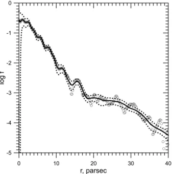
Spatial radial density profiles were derived in the present work with the use of equations (9) and (10) for the sameN-body model outputs. The adaptive kernel algorithm was used, because the outer part of the cluster model corona has a very low density. The se-lection of the optimal kernel half-width was made following the recommendations of Merritt & Tremblay (1994). Fig.5shows the spatial density profiles of the open-cluster corona model 1 from Danilov & Dorogavtseva (2008) at the time-point of about 150 Myr (about three violent relaxation times of the model), obtained with different kernel half-widths (0.5, 1, 2, 3, 4 and 5 pc from top to bot-tom). The half-width mentioned everywhere in this section is the one used in the pilot estimate for the adaptive kernel method. The stochasticity of the plots in the central region of the cluster is caused by small values of factorsλ, which control the kernel half-width in the adaptive kernel algorithm (λ <1 forr<10 pc). For this reason, factorsλwere restricted in the present work by 1 from the lower side in the case of spatial density determination.
Fig.6shows the comparison of fixed and adaptive kernel esti-mates with the kernel half-widthh=1 pc (in the case of the adaptive kernel estimator,h=1 pc refers to the pilot estimate). The adaptive kernel estimate was made with the restricted factorsλ. The solid line in this figure shows the adaptive kernel estimate of the spatial density in the corona of model 1 from Danilov & Dorogavtseva (2008) at the time-point of about 150 Myr in units of pc−3. The tidal
Figure 6. Comparison of the adaptive and fixed kernel estimates of spatial density of the open-cluster corona model. The solid line is the adaptive estimate, the dotted lines show the confidence interval of 2σwidth and the open circles show the fixed kernel estimate. The kernel half-width is 1 pc. In the case of the adaptive kernel estimator, it is the kernel half-width for the pilot estimate. The time-point is about 150 Myr.
radius of this model in the Galactic gravitational field is about 10 pc (see the formula for the tidal radius in Section 7). The dashed lines show the confidence interval of 2σwidth obtained by the smoothed bootstrap method (see Merritt & Tremblay1994). This method is based on the Monte Carlo simulation of multiple secondary sam-ples. Secondary samples are created, which are equal to the original one in size, and are distributed in accordance with the same density distribution as the original sample. Then, the density estimate for every secondary sample is obtained, using the same kernel estima-tor. In this work, 20 secondary samples were used; this gave density dispersion values for everyripoint. The fixed kernel estimate is shown by open circles. It is clear that the adaptive kernel estimate withh=1 pc follows the mean trend defined by the fixed kernel estimate withh=1 pc, and is relatively smooth. The adaptive kernel estimate withh=2 pc has the same characteristics, but is smoother in the central region. Adaptive estimates withh= 3, 4 and 5 pc are biased in the outer part of the corona model. Thus, the kernel half-widths of 1 and 2 pc were selected for estimation of spatial density of the open-cluster corona model.
The evolution of the spatial density profile with time for the corona of cluster model 1 (Danilov & Dorogavtseva2008) is shown
in the sequences of frames ‘spatial density 1.flv’ (the kernel half-width of 1 pc) and ‘spatial density 2.flv’ (the kernel half-half-width of 2 pc), which are accessible as supporting information in the online version of this paper. Each frame is arranged as in Fig.6, but with-out the comparison with the fixed kernel estimate. Each sequence contains 60 frames, and the time interval is about 0.05 of the violent relaxation time of this model (Danilov & Dorogavtseva2008); that is, about 2.5 Myr. The last frame in ‘spatial density 1.flv’ is the same as Fig.6. It can be observed that an imaginary upper envelope line for the density profile is stretched to about three tidal radii of the model. This confirms the results of Danilov et al. (2014) on the formation of the quasi-equilibrium density distribution in the cluster corona models. It means that the density profile approaches, with time, the upper envelope line, which is just the quasi-equilibrium density distribution. This temporal equilibrium in the corona indi-cates a balance between the numbers of stars entering the corona from inner regions of the cluster and those escaping to the corona periphery or beyond it (Danilov et al.2014).
4 S U R FAC E D E N S I T Y P R O F I L E S F O R O P E N C L U S T E R S
Surface density profiles for seven open clusters were obtained in this work for different limiting magnitudes,Jlim, with the data of the Two-Micron All-Sky Survey (2MASS; Skrutskie et al2006). The sample clusters are listed in Table1. This table shows the galac-tic coordinates of clusters, their colour excesses, distance modules, distances and ages taken from Loktin, Gerasimenko & Malysheva (2001), with the lastest correction of the data (Loktin 2012, pri-vate communication). With the exception of NGC 1960, all sample clusters were selected at large galactic latitudes in order to have a more uniform and relatively low stellar background density. Two clusters are young, two clusters are intermediate-aged and three clusters are old. The cluster centre coordinates were taken from the WEBDA data base (Netopil, Paunzen & St¨utz2012); their accuracy was found to be sufficient for the large kernel half-width used in this work (usually 5 or 10 arcmin).
The case for real open clusters is very different from the case for open-clusterN-body models. Real clusters are observed at the rich stellar background, and the range of the estimates of the surface density values in this case is much smaller than the range of the estimates of the spatial (or surface) density for the models. For this reason, the factorsλ, which adjust the kernel half-width in the adaptive kernel algorithm, also have a small range for the real clusters. Factorsλdiffer from unity noticeably only in the region of the cluster core. As a result, the adaptive and the fixed kernel estimates of the surface density differ only in the region of the cluster core and coincide completely in the region of the cluster halo and corona. The present work is aimed generally at the study Table 1. Sample clusters.
Cluster name l b E(B−V) Dist. mod. Distance Log age h Rf
(deg) (deg) (mag) (mag) (pc) (arcmin) (arcmin)
NGC 1502 143.6 7.6 0.76±0.01 9.60± 0.14 830±50 7.04±0.05 10 110 NGC 1960 (M36) 174.5 1.0 0.23±0.04 10.59± 0.10 1310±60 7.42±0.20 5 60 NGC 2287 (M41) 231.1 −10.2 0.03±0.01 9.21± 0.10 700±30 8.39±0.07 10 120 NGC 2516 273.9 −15.9 0.10±0.01 8.10± 0.11 420±20 8.10±0.04 10 110 NGC 2682 (M67) 215.6 31.7 0.06±0.01 9.79± 0.05 910±20 9.41±0.02 5 115 NGC 6819 74.0 8.5 0.24±0.04 11.87± 0.20 2360±200 9.17±0.07 5 55 NGC 6939 95.9 12.3 0.33±0.03 10.45± 0.36 1230±200 9.35±0.05 10 160
Figure 7. Surface density profiles of open cluster NGC 2287, obtained with different kernel half-width values forJlim=13 mag: (a)h=2 arcmin; (b)
h=3 arcmin; (c)h=5 arcmin; (d)h=10 arcmin; (e)h=15 arcmin; (f)h
=20 arcmin; (g)h=30 arcmin. The ordinate is the surface density in the units of arcmin−2, and the abscissa is the distance from the cluster centre
in arcmin. The thick solid line shows the surface density kernel estimate and the dotted lines show the confidence interval of 2σwidth, obtained by a smoothed bootstrap method.
of the outer regions of the open clusters, and for this reason the fixed kernel algorithm is used in the present work to estimate the surface density of the open clusters.
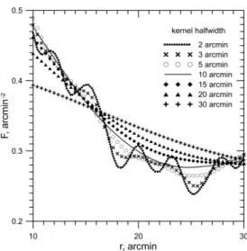
Let us examine how the result of the surface density estimation depends on the kernel half-widthh. Fig.7shows the radial surface density profiles for cluster NGC 2287 forJlim=13 mag, obtained with different kernel widths. It is seen that when the kernel half-width decreases, the variation of the profile increases. Figs7(a)–(c) vary too much. It is difficult to estimate the degree of bias, because at the background region (r>60 arcmin) all kernel half-widths give the same estimate of background density value. A comparison of the surface density estimates in the region where the density gradient is changing considerably (the outer part of the cluster core) is the best way to estimate the degree of bias in that case. Fig.8shows the surface density estimates for NGC 2287 obtained with different kernel half-widths in the distance ranger∈[10, 30] arcmin. It is seen that the curve with h= 10 arcmin is smooth, and follows well the mean trend defined by the curves computed with a much
Figure 8. Surface density profiles of open cluster NGC 2287, obtained with different kernel half-width values forJlim=13 mag in the transition
region between the cluster core and the cluster halo. The different symbols correspond to the different values of the kernel half-width.
smaller smoothing parameter. The curves with larger kernel half-widths deviate from this trend appreciably. Then, the best value of the kernel half-width in this case is 10 arcmin, in accordance with the recommendations of Merritt & Tremblay (1994).
The same procedure was applied to all sample clusters for all values of the limiting magnitude. One value of the kernel half-width was selected for every cluster, with the aim of comparing the surface density estimates derived with different limiting magnitudes. The last two columns of Table1show, respectively, the kernel half-width hvalues accepted for the construction of the surface density radial profiles of the sample clusters, and the radiiRfof the fields under consideration. (It is important to note that in order to estimate the surface density using the kernel estimator with the kernel half-width hinside the circle of radiusRf, the coordinates of stars inside the circle with radiusRf+hare needed.)
Tables2–8contain data on the surface density profiles obtained in this work; each table contains data for one cluster. The full versions of all these tables are accessible as supporting information in the online version of this paper. All tables are organized in a similar way, as follows. The first column contains the distance from the cluster centre in arcmin. Columns 2–5 contain data for the limiting magnitudeJlim =11 mag: column 2 is the kernel estimate of the surface density radial profile with the kernel half-width listed in Table1; column 3 is the lower boundary of the confidence interval; column 4 is the upper boundary of the confidence interval; column 5 is the surface density histogram with the bin width of 4 arcmin. Histograms with the same bin width are tabulated for all clusters (a comparison of kernel estimates and histograms could be useful in some cases). Columns 6–9 contain the same data for the limiting magnitudeJlim =12 mag; columns 10–13 contain the same data for the limiting magnitudeJlim=13 mag; columns 14–17 contain the same data for limiting magnitudeJlim=14 mag; columns 18– 21 contain the same data for limiting magnitudeJlim =15 mag; columns 22–25 contain the same data for limiting magnitudeJlim= 16 mag. All surface density data are in units of arcmin−2.
The surface density radial profiles for different limiting magni-tudes are used in the present work to estimate the cluster masses, and to evaluate the segregation of the stars with the different masses (mass segregation).
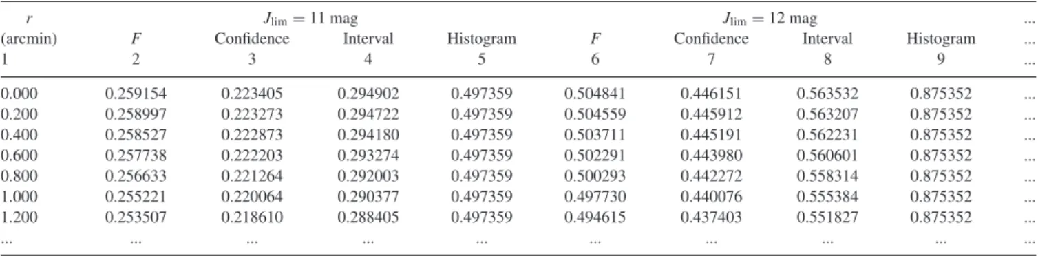
Table 2. Data on surface density radial profiles for NGC 1502: the first nine columns and the first seven rows are shown (the full table is accessible in the online version of this paper).
r Jlim=11 mag Jlim=12 mag ...
(arcmin) F Confidence Interval Histogram F Confidence Interval Histogram ...
1 2 3 4 5 6 7 8 9 ... 0.000 0.259154 0.223405 0.294902 0.497359 0.504841 0.446151 0.563532 0.875352 ... 0.200 0.258997 0.223273 0.294722 0.497359 0.504559 0.445912 0.563207 0.875352 ... 0.400 0.258527 0.222873 0.294180 0.497359 0.503711 0.445191 0.562231 0.875352 ... 0.600 0.257738 0.222203 0.293274 0.497359 0.502291 0.443980 0.560601 0.875352 ... 0.800 0.256633 0.221264 0.292003 0.497359 0.500293 0.442272 0.558314 0.875352 ... 1.000 0.255221 0.220064 0.290377 0.497359 0.497730 0.440076 0.555384 0.875352 ... 1.200 0.253507 0.218610 0.288405 0.497359 0.494615 0.437403 0.551827 0.875352 ... ... ... ... ... ... ... ... ... ... ...
Table 3. Data on surface density radial profiles for NGC 1960: the first nine columns and the first seven rows are shown (the full table is accessible in the online version of this paper).
r Jlim=11 mag Jlim=12 mag ...
(arcmin) F Confidence Interval Histogram F Confidence Interval Histogram ...
1 2 3 4 5 6 7 8 9 ... 0.000 0.494103 0.408144 0.580063 0.716197 0.847316 0.699692 0.994941 1.114085 ... 0.200 0.493111 0.407407 0.578815 0.716197 0.846140 0.698862 0.993417 1.114085 ... 0.400 0.490031 0.405061 0.575002 0.716197 0.842446 0.696186 0.988706 1.114085 ... 0.600 0.484854 0.401084 0.568624 0.716197 0.836177 0.691566 0.980787 1.114085 ... 0.800 0.477629 0.395503 0.559755 0.716197 0.827532 0.685107 0.969957 1.114085 ... 1.000 0.468473 0.388420 0.548526 0.716197 0.816571 0.676838 0.956305 1.114085 ... 1.200 0.457641 0.380069 0.535213 0.716197 0.803530 0.666959 0.940100 1.114085 ... ... ... ... ... ... ... ... ... ... ...
Table 4. Data on surface density radial profiles for NGC 2287: the first nine columns and the first seven rows are shown (the full table is accessible in the online version of this paper).
r Jlim=11 mag Jlim=12 mag ...
(arcmin) F Confidence Interval Histogram F Confidence Interval Histogram ...
1 2 3 4 5 6 7 8 9 ... 0.000 0.241070 0.202440 0.279701 0.298416 0.390958 0.352763 0.429154 0.437676 ... 0.400 0.240801 0.202263 0.279340 0.298416 0.390638 0.352573 0.428702 0.437676 ... 0.800 0.239993 0.201714 0.278272 0.298416 0.389702 0.352038 0.427367 0.437676 ... 1.200 0.238641 0.200780 0.276503 0.298416 0.388154 0.351152 0.425156 0.437676 ... 1.600 0.236728 0.199417 0.274038 0.298416 0.385998 0.349891 0.422104 0.437676 ... 2.000 0.234303 0.197672 0.270933 0.298416 0.383300 0.348294 0.418306 0.437676 ... 2.400 0.231431 0.195608 0.267254 0.298416 0.380169 0.346434 0.413905 0.437676 ... ... ... ... ... ... ... ... ... ... ...
Table 5. Data on surface density radial profiles for NGC 2516: the first nine columns and the first seven rows are shown (the full table is accessible in the online version of this paper).
r Jlim=11 mag Jlim=12 mag ...
(arcmin) F Confidence Interval Histogram F Confidence Interval Histogram ...
1 2 3 4 5 6 7 8 9 ... 0.000 0.349702 0.313795 0.385609 0.457570 0.519434 0.450923 0.587945 0.696303 ... 0.200 0.349571 0.313690 0.385453 0.457570 0.519229 0.450760 0.587698 0.696303 ... 0.400 0.349182 0.313378 0.384986 0.457570 0.518618 0.450277 0.586959 0.696303 ... 0.600 0.348547 0.312871 0.384224 0.457570 0.517615 0.449490 0.585740 0.696303 ... 0.800 0.347680 0.312178 0.383182 0.457570 0.516236 0.448419 0.584053 0.696303 ... 1.000 0.346592 0.311314 0.381871 0.457570 0.514490 0.447072 0.581909 0.696303 ... 1.200 0.345289 0.310278 0.380300 0.457570 0.512390 0.445455 0.579325 0.696303 ... ... ... ... ... ... ... ... ... ... ...
Table 6. Data on surface density radial profiles for NGC 2682: the first nine columns and the first seven rows are shown (the full table is accessible in the online version of this paper).
r Jlim=11 mag Jlim=12 mag ...
(arcmin) F Confidence Interval Histogram F Confidence Interval Histogram ...
1 2 3 4 5 6 7 8 9 ... 0.000 0.335090 0.245409 0.424772 0.338204 0.948296 0.798863 1.097728 0.875352 ... 0.200 0.334626 0.245181 0.424072 0.338204 0.947063 0.798132 1.095994 0.875352 ... 0.400 0.333231 0.244464 0.421997 0.338204 0.943360 0.795906 1.090815 0.875352 ... 0.600 0.330808 0.243141 0.418476 0.338204 0.936956 0.791902 1.082010 0.875352 ... 0.800 0.327318 0.241154 0.413482 0.338204 0.927699 0.785880 1.069519 0.875352 ... 1.000 0.322784 0.238516 0.407052 0.338204 0.915598 0.777725 1.053471 0.875352 ... 1.200 0.317302 0.235290 0.399313 0.338204 0.900800 0.767483 1.034116 0.875352 ... ... ... ... ... ... ... ... ... ... ...
Table 7. Data on surface density radial profiles for NGC 6819: the first nine columns and the first seven rows are shown (the full table is accessible in the online version of this paper).
r Jlim=11 mag Jlim=12 mag ...
(arcmin) F Confidence Interval Histogram F Confidence Interval Histogram ...
1 2 3 4 5 6 7 8 9 ... 0.000 0.859398 0.750552 0.968244 1.591549 1.263490 1.087194 1.439786 2.307747 ... 0.200 0.857808 0.749343 0.966272 1.591549 1.261203 1.085338 1.437068 2.307747 ... 0.400 0.852799 0.745457 0.960140 1.591549 1.254023 1.079488 1.428558 2.307747 ... 0.600 0.844158 0.738621 0.949696 1.591549 1.241678 1.069404 1.413951 2.307747 ... 0.800 0.831955 0.728846 0.935064 1.591549 1.224336 1.055251 1.393421 2.307747 ... 1.000 0.816190 0.716070 0.916309 1.591549 1.202229 1.037226 1.367232 2.307747 ... 1.200 0.796959 0.700322 0.893595 1.591549 1.175547 1.015433 1.335661 2.307747 ... ... ... ... ... ... ... ... ... ... ...
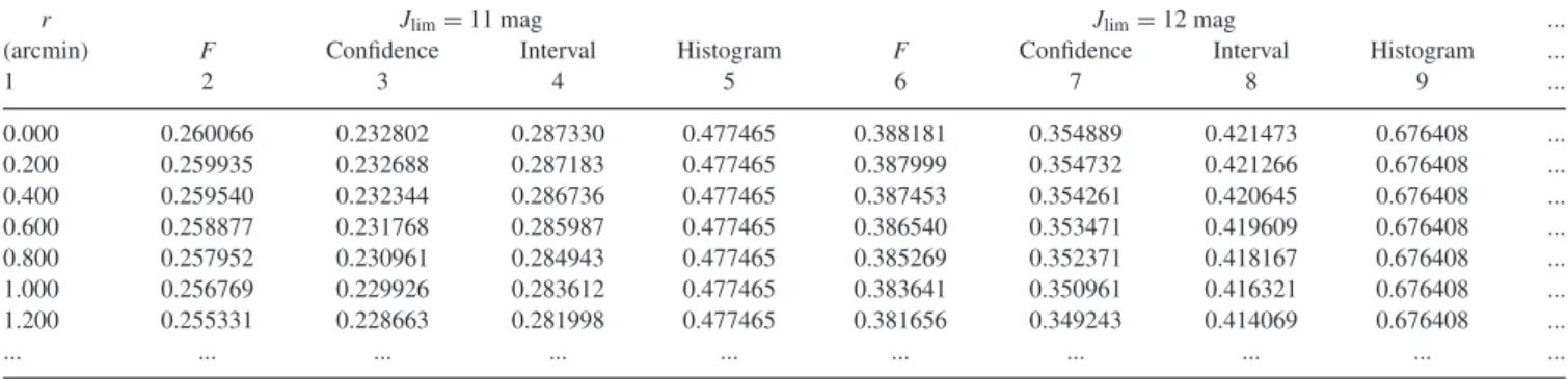
Table 8. Data on surface density radial profiles for NGC 6939: the first nine columns and the first seven rows are shown (the full table is accessible in the online version of this paper).
r Jlim=11 mag Jlim=12 mag ...
(arcmin) F Confidence Interval Histogram F Confidence Interval Histogram ...
1 2 3 4 5 6 7 8 9 ... 0.000 0.260066 0.232802 0.287330 0.477465 0.388181 0.354889 0.421473 0.676408 ... 0.200 0.259935 0.232688 0.287183 0.477465 0.387999 0.354732 0.421266 0.676408 ... 0.400 0.259540 0.232344 0.286736 0.477465 0.387453 0.354261 0.420645 0.676408 ... 0.600 0.258877 0.231768 0.285987 0.477465 0.386540 0.353471 0.419609 0.676408 ... 0.800 0.257952 0.230961 0.284943 0.477465 0.385269 0.352371 0.418167 0.676408 ... 1.000 0.256769 0.229926 0.283612 0.477465 0.383641 0.350961 0.416321 0.676408 ... 1.200 0.255331 0.228663 0.281998 0.477465 0.381656 0.349243 0.414069 0.676408 ... ... ... ... ... ... ... ... ... ... ...
The nominal completeness limit of the 2MASS Point Source Catalogue is 15.8 mag (Skrutskie et al2006), but in the magnitude rangeJ∈[15.8, 16.0] mag this catalogue is 99 per cent complete for virtually all of the sky (Cutri et al.2003). At the same time, the completeness limit is∼0.9 mag fainter at high galactic latitude and ∼0.4 mag brighter in the galactic plane (Cutri et al.2003). This means that the completeness limit varies depending on the overall stellar density, and the completeness in the last magnitude range (Jlim=16 mag) can be less than unity and different from one cluster to another.
It can be seen from the results of Merritt & Tremblay (1994) that both the kernel and maximum likelihood methods overestimate the surface density in the region of the outer boundary when large values of the smoothing parameter (the kernel half-width) are used for the restoration of the Plummer and Michie–King distributions. In that case, it is probable that a larger kernel half-width would lead to larger cluster dimensions.
The real open clusters do not show noticeable dependence of the cluster radius on the kernel half-width, when the kernel half-widths listed in Table1and smaller values are used. A possible explanation is that the open clusters are projected on a rich stellar background, as opposed to the Merritt & Tremblay (1994) models where the stellar background is not taken into account. This is illustrated in Fig.9. Fig.9(a) shows surface density profiles in the region around the cluster boundary for cluster NGC 2287 forJlim=13 mag, for kernel half-width values of 2, 3, 5 and 10 arcmin. Fig.9(b) shows surface density profiles in the region around the cluster boundary for cluster NGC 6819 forJlim = 16 mag, for kernel half-width values of 2, 3 and 5 arcmin. The cluster boundary (the value of the cluster radius) is determined by the intersection of the cluster surface density profile, obtained with the kernel half-width listed in Table1and marked in Fig.9by the thick solid lines, with the line of background density (the dashed line; see the explanation in Section 5). It is clearly noted that the intersection points of the other
Figure 9. Surface density profiles of the clusters in the region around the cluster boundary, obtained with the different kernel half-width values: (a) NGC 2287,Jlim=13 mag; (b) NGC 6819,Jlim=16 mag. Different
sym-bols correspond to different values of the kernel half-width. The horizontal dashed line shows the visual estimate of background density (see explana-tion in Secexplana-tion 5). Grey bands show the 2σconfidence intervals for profiles with (a)h=10 arcmin and (b)h=5 arcmin.
surface density profiles (obtained with the smaller kernel half-width values) with the background density line – near 46–47 arcmin in Fig.9(a) and near 22–23 arcmin in Fig.9(b) – are inside the bands of the confidence interval for profiles with the kernel half-width values from Table1(the larger values).
The density profiles obtained with different limiting magnitudes were compared in the present work in order to find signs of mass segregation in the sample clusters. As the surface density values differ greatly for different limiting magnitudes, relative densities were used, determined by
Frel(ri)= F(ri)−F vis b F(0)−Fvis b , (11) whereFvis
b is the visual estimate of the surface density of the stellar background (see the explanation in Section 5) andF(0) is the surface density in the cluster centre.
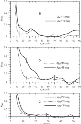
A comparison of the relative density profiles for clusters NGC 1502, 2516 and 6819 is shown in Figs10(a), (b) and (c), respectively. Two types of differences can be seen. The first is presented in all three clusters: the outer part of the cluster core (or ‘intermediate
Figure 10. Comparison of relative surface density profiles for different limiting magnitudes: (a) NGC 1502; (b) NGC 2516; (c) NGC 6819. Vertical bars show the width of the 2σconfidence interval.
zone’) is relatively more populous in faint stars. The second type is seen in the case of NGC 2516, where the cluster halo is also more populous in faint stars. All sample clusters show differences of one type or the other. In all cases, the relative population of faint stars in the outer cluster regions exceeds the relative population of brighter stars, apart from NGC 6819, where the opposite can be seen (Fig.10c).
The Kolmogorov–Smirnov (KS) test was performed in order to statistically compare the relative density profiles in Fig.10(Press et al.1992). For the profiles from Fig.10(a) and (b), the KS test givesp-values of 3.8×10⁻³and 3.4×10⁻¹⁰, respectively (i.e. these profiles are statistically different). For the profiles from Fig.10(c), the KS test gives the following results. The profiles withJlim = 12 and 13 mag are not statistically different (the corresponding p-value is 0.9999). The profiles withJlim =12 and 16 mag are statistically different (the correspondingp-value is 4.1×10⁻⁷). The profiles withJlim =13 and 16 mag are also statistically different (the correspondingp-value is 1.3×10⁻⁶).
The mass of sample cluster stars for different magnitudes can be estimated. Transition to absolute magnitudesMJwas made with
the data on cluster distances and colour excessesE(B−V) from the Loktin et al. (2001) catalogue and with the use of the following formulae:
E(J−H)=0.37E(B−V); (12) AJ=2.43E(J−H). (13) Here,E(J−H) is the colour excess in the (J−H) colour index andAJis the total extinction inJcolour. Equation (12) was taken from Bessell & Brett (1988), and equation (13) from Laney & Stobie (1993). Then, the masses of stars were estimated by their
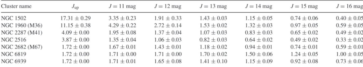
Table 9. Stellar masses at the boundaries of magnitude intervals in the sample clusters (M). Here,Jupis the magnitude of the upper end of the cluster
sequence in the CMD (see explanation in the text).
Cluster name Jup J=11 mag J=12 mag J=13 mag J=14 mag J=15 mag J=16 mag
NGC 1502 17.31±0.29 3.35±0.23 1.91±0.33 1.43±0.03 1.15±0.05 0.74±0.06 0.40±0.05 NGC 1960 (M36) 11.15±0.38 4.29±0.22 2.72±0.14 1.53±0.02 1.32±0.03 0.97±0.05 0.59±0.05 NGC 2287 (M41) 4.09±0.00 1.95±0.08 1.37±0.04 1.07±0.03 0.83±0.03 0.65±0.02 0.49±0.02 NGC 2516 3.87±0.00 1.35±0.04 1.06±0.03 0.82±0.03 0.64±0.02 0.49±0.02 0.33±0.02 NGC 2682 (M67) 1.72±0.00 1.67±0.01 1.43±0.01 1.18±0.02 0.94±0.01 0.74±0.01 0.59±0.01 NGC 6819 1.72±0.00 1.71±0.00 1.71±0.00 1.70±0.02 1.50±0.06 1.24±0.05 1.00±0.05 NGC 6939 1.72±0.00 1.71±0.01 1.65±0.08 1.41±0.10 1.15±0.09 0.92±0.08 0.73±0.06 absolute magnitudes MJ with isochrone tables downloaded from
http://stev.oapd.inaf.it/cmd(Bressan et al.2012) withZ =0.019. The isochrone of lgt=7.0 was used for clusters NGC 1502 and 1960; the isochrone of lgt=8.3 was used for clusters NGC 2287 and 2516; the isochrone of lgt=9.3 was used for clusters NGC 2682, 6819 and 6939. One isochrone is used for the young clusters, one isochrone for the intermediate-aged clusters and one isochrone for the old clusters. The reason for this is that only the mass– luminosity relation is important in the present work, and this relation changes only negligibly for isochrones with close age values. It is important that this method does not require the matching of the isochrone to the cluster colour–magnitude diagram (CMD).
The data on stellar masses corresponding to stellar magnitudes in the sample clusters are listed in Table9, whereJupdenotes the magnitude of the upper end of the cluster sequence in the CMD. In order to find this value, the CMDs [J, (J− H)] for sample clusters were plotted by the data of the 2MASS in the region of 10 arcmin around the cluster centre. The uncertainties in this table are a result of uncertainties in the cluster distance modules, and in the colour excesses for the clusters (see Table 1). Where the uncertainty interval was determined as asymmetric, the larger value is listed.
The differences in the relative density profiles with the different limiting magnitudes are present in all sample clusters. It is seen from Table9that, at least in the young and intermediate-age clusters, there is a large mass spectrum; so, we can explain the differences in the profiles there as the consequence of a mass segregation process. For NGC 6819, the outer part of the cluster core is more populated with faint stars, but the cluster halo is more populous with the brighter stars. However, the difference in the mass between cluster stars in that case is minimal, and this fact has yet to be interpreted.
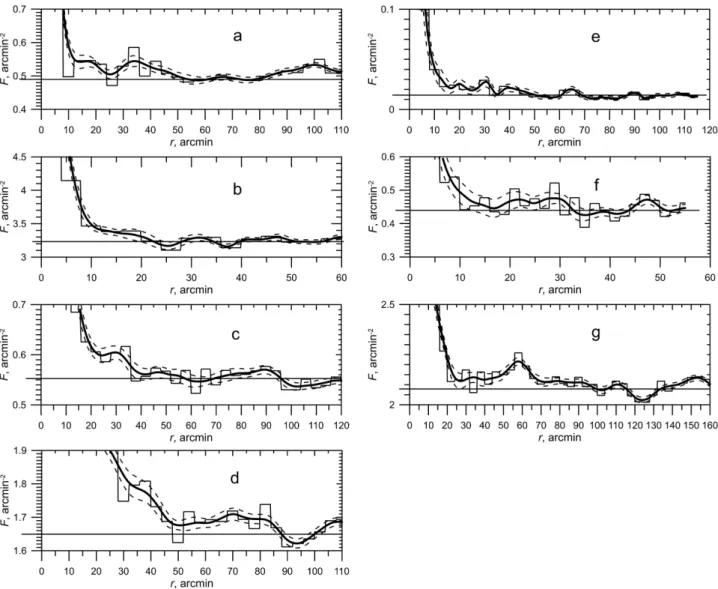
The sample clusters show the presence of structural irregularities in their density profiles, such as secondary maxima or ‘footsteps’ (a ‘footstep’ is the same as a ‘plateau’). The only exception is NGC 1960. Examples are shown in Fig.11. A typical ‘footstep’ is seen in NGC 2287 nearr=30 arcmin, and a typical secondary maximum is seen in NGC 6939 nearr=60 arcmin. Such structures can indicate cluster non-stationarity in the regular field, or stabilizing ejections of the cluster stars into the galactic field (see Danilov1982,2005, 2011). The non-stationary processes cause the corona to be not radially symmetric, and this, in turn, leads again to the structural irregularities in the radial density profiles.
5 S I Z E S O F O P E N C L U S T E R S
The sizes of open clusters were estimated in the present work in two ways. The first was by a visual estimate, and it was not an objective method.
In the first step, the mean background surface density line was inferred by analysing the outer part of the field under
considera-tion for every cluster, and for every limiting magnitude range. An approximately flat area in the outer part of the density profile was searched, and the background density line was drawn, taking into account an approximate equality of the square of areas between this line and the density profile above and below this line. In the second step, the cluster radius was estimated as the abscissa of the point of intersection of the density profile and the background density line. An error of this estimate was evaluated as the distance from the intersection point of the confidence interval line with the back-ground density line to the cluster radius point (in many cases, the confidence interval intersects the background density line only at one side of the cluster radius point). An error of the background density estimate was evaluated as half of the confidence interval width at the cluster radius point.
These background density lines are shown in Figs9and11. The visual estimates of the cluster radius Rc and the surface density of stellar backgroundFvis
b , and their uncertainties for every cluster and every limiting magnitude interval are listed in Table11. The intervals of the cluster radius estimates for every cluster are listed in the second column of Table10.
The second way is the approximation of the cluster surface den-sity profile by the King surface denden-sity distribution (King1962), and by the combination of the King distribution and the cluster corona component (see the description and the discussion in Sec-tion 6). It is important that the visual estimates of the mean back-ground surface density and the estimates of the backback-ground density via approximation with the combined function are very close (see Table11).
Table10shows the comparison of visual estimates of open-cluster radii, both with the data of other authors and with the results of cluster radii estimation by the DMP method when the functionN(r) (i.e. the number of stars in the circle with radiusr) is used, and the cluster field is compared with several fields of neighbouring background fields (see the introduction). All data in Table10are in arcmin.
The second column of Table10contains the visual estimates of cluster radius by the surface density profile obtained as described above. The interval shows the scatter of the estimates for the dif-ferent limiting magnitudes. The number in brackets is the radius of the field used for the density profile construction. The third column shows the cluster radius from the catalogue of Kharchenko et al. (2005). The fourth column shows the data on the sample clusters from the literature, and the fifth column contains the references for the sources of these data. The sixth column contains the cluster radius estimates from Danilov & Seleznev (1994). These estimates were obtained by the DMP method with star counts on photographic plates in the B colour band. The number in brackets shows the radius of the cluster field used for the star counts. The seventh column shows the cluster radius estimates obtained by the DMP method with the star counts on the data of 2MASS. The interval
Figure 11. Structural irregularities in the surface density profiles of open clusters: (a) NGC 1502,Jlim=14 mag; (b) NGC 1960,Jlim=16 mag; (c) NGC
2287,Jlim=14 mag; (d) NGC 2516,Jlim=16 mag; (e) NGC 2682,Jlim=11 mag; (f) NGC 6819,Jlim=13 mag; (g) NGC 6939,Jlim=16 mag. The
solid polygonal lines show the histograms with the bin size of 4 arcmin. The thick solid lines show the surface density estimate and the dashed lines show a confidence interval of 2σwidth. The solid straight lines show the values of stellar density of the background (see explanation in Section 5).
Table 10. Comparison of cluster radii estimates with the data of other authors and with the results of cluster radii estimation by the DMP method (arcmin).
Cluster radius Kharchenko Data of Danilov & Seleznev Radii estimates
estimate by et al. (2005) other (1994) DMP method by DMP method
Cluster name density profile catalogue authors Ref.a with plates inB with 2MASS
NGC 1502 52–55 (110) 12.6 5 1 24.8±2.5 (31.08) 37 (45) NGC 1960 (M36) 10–23 (60) 16.2 22.9 2 20.1±0.6 (31.08) NGC 2287 (M41) 37–57 (120) 30 30 3 46–50 (60) NGC 2516 88–92 (110) 42 90 3 87 (95) NGC 2682 (M67) 43–57 (115) 18.6 60 4,5 NGC 6819 16–33 (55) 13 6 24.8±2.6 (31.08) 10–22 (40) NGC 6939 42–105 (160) 85 7 15.5±1.2 (22.2) 21–26 (30)
Notes.aReferences are: (1) Alves et al. (2012); (2) Sanchez & Alfaro (2009); (3) Bergond, Leon & Guibert (2001); (4) Davenport & Sandquist (2010); (5) Balaguer-N´u˜nez et al. (2013); (6) Yang et al. (2013); (7) Artyukhina & Kholopov (1965).
shows the scatter of estimates for different limiting magnitudes, and the number in a brackets shows the radius of the cluster field used for the star counts.
The radius estimates by the surface density profile for NGC 1502, 6819 and 6939 are larger than estimates by star counts with the DMP
method. This can be explained by a smaller size of the cluster field used for the DMP star counts. For NGC 1960, 2287 and 2516, the size of the field used for the star counts with the DMP method is larger than the cluster size, and a satisfactory matching by different methods was obtained.
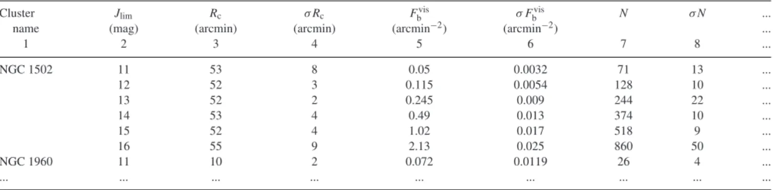
Table 11. Approximation of the surface density profiles of the sample clusters: the first eight columns and the first seven rows are shown (the full table is accessible in the online version of this paper).
Cluster Jlim Rc σRc Fbvis σ Fbvis N σN ...
name (mag) (arcmin) (arcmin) (arcmin−2) (arcmin−2) ...
1 2 3 4 5 6 7 8 ... NGC 1502 11 53 8 0.05 0.0032 71 13 ... 12 52 3 0.115 0.0054 128 10 ... 13 52 2 0.245 0.009 244 22 ... 14 53 4 0.49 0.013 374 10 ... 15 52 4 1.02 0.017 518 9 ... 16 55 9 2.13 0.025 860 50 ... NGC 1960 11 10 2 0.072 0.0119 26 4 ... ... ... ... ... ... ... ... ... ...
It can be seen from Table10that, for NGC 1502, 2287 and 6819, we have in the literature underestimated values of the cluster radius. Artyukhina & Kholopov (1965) studied the structure of NGC 6939 with the proper-motion-selected cluster members. They found that this cluster has an extensive corona with the radius of about 85 arcmin. In the present work, the surface density profile for NGC 6939 was derived to a distance of 160 arcmin from the cluster centre, and a cluster radius estimate larger than in Artyukhina & Kholopov (1965) was obtained (see Fig.11g). In this manner, the result of Artyukhina & Kholopov (1965) concerning an extensive corona of NGC 6939 can be confirmed. The cluster radius estimate, comparable with the result of proper-motion cluster membership analysis, was obtained for NGC 2682 (Balaguer-N´u˜nez et al.2013). Kharchenko et al. (2005) used proper-motion data for selecting possible cluster members, but they obtained smaller cluster radii than in the present work. This is possibly because of the smaller limiting magnitude in their study, and possibly as a result of using the King (1962) distribution for the cluster structure approximation (see discussion in Section 6).
Nilakshi, Pandey & Mohan (2002) performed star counts in the fields of 38 open clusters. They obtained an outer radius for NGC 1960 of 15.3 arcmin and an outer radius for NGC 6939 of 12.7 arcmin (these values of angular radii were calculated with their data on linear radii and distances). These radii are smaller than the ones obtained in the present paper. For NGC 6939, Nilakshi et al. (2002) could not see the cluster boundary near 100 arcmin, because they were limited by the field with a radius of 30 arcmin. Their result must be compared with the Danilov & Seleznev (1994) value (see column 6 of Table10). For NGC 1960, the reason for the underestimation of the radius by Nilakshi et al. (2002) is pos-sibly the lower sensitivity of star counts in the rings in compari-son with the kernel estimator method. It is worth noting that the procedure of the outer boundary determination was not described by Nilakshi et al. (2002) in detail, and the density profiles (see fig.1in Nilakshi et al.2002) allow an ambiguous estimation of the radii.
6 A P P R OX I M AT I O N O F O P E N - C L U S T E R S U R FAC E D E N S I T Y P R O F I L E S
The King (1962) function is very often used for approximation of the surface density or the surface brightness profiles of star clusters:
F(r)= ⎧ ⎪ ⎪ ⎪ ⎨ ⎪ ⎪ ⎪ ⎩ k 1 1+(r/rc)2− 1 1+(rt/rc)2 2 r < rt, 0 r≥rt. (14)
This function was proposed by King for globular clusters but was also widely used for open clusters. In order to take into account stel-lar background, this formula is supplemented by stelstel-lar background densityFbas a constant addition.
Danilov & Putkov (2012) found that the approximation of stellar distribution in open star clusters by the King (1962) function tends to underestimate the number of stars in the cluster compared to the results of star counts. The reason for this is that the King (1962) function underestimates density values in the region of the cluster corona. Danilov & Putkov (2012) proposed an addition to the King formula. This addition represents the cluster corona as a uniform sphere. The addition into surface density is
δF(r)=2R2δf 1− r R2 2 , (15)
whereR2is the radius of the cluster corona andδfis the spatial density of the cluster corona. This addition should be applied at all radiir<R2.
An approximation of the surface density profiles of the sample clusters was performed in the present work, both using the King (1962) function alone (equation 14, referred to hereafter as the ‘King model’) and using the combined function (a combination of the King distribution for the cluster core equation 14 and of the uniform sphere equation 15 for the cluster corona, referred to hereafter as the ‘combined model’).
The results of the approximation are listed in Table11, which is accessible in the online version of this paper. The columns of the table can be divided into three groups. The first group contains visual estimates of the cluster parameters, the second group contains the parameters of the combined model and the third group contains the parameters of the King model.
The columns of the first group are: (1) the cluster name; (2) the limiting magnitude in the Jband; (3) visual estimate of the cluster radiiRc in arcmin; (4) its uncertainty; (5) visual estimate of the surface density of the stellar backgroundFvis
b in arcmin−2; (6) its uncertainty; (7) the estimate of the cluster star numberN; (8) its uncertainty. The estimate of the cluster star number was obtained through the numerical integration of the cluster surface density profile; the uncertainty of this estimate was obtained by integration of the upper and lower confidence interval curves, taking into account the uncertainty in the background density.
The parameters of the combined model were obtained by using the non-linear least-squares approximation algorithm by Marquardt (1963). The parameters of equation (14) for the combined model are supplied by the superscript ‘comb’, and for the King model by the superscript ‘King’. The columns of the second group are: (9)
kcombin arcmin−2; (10) its uncertainty; (11) rcomb
c in arcmin; (12) its uncertainty; (13)rcomb
t in arcmin; (14) its uncertainty; (15) the surface density of backgroundFcomb
b in arcmin−
2; (16) its uncer-tainty; (17)R2in arcmin; (18) its uncertainty; (19)δfin units of 10−3arcmin−3(this value denotes the number of stars in a cube with the side measured by one arcmin at the cluster distance); (20) its uncertainty. In the combined model,rcomb
t can be considered as the cluster core radius,rcomb
c has the meaning of the scale parameter for the cluster core andR2is the cluster corona radius. From this per-spective, situations whenrcomb
c > r comb
t are possible (see Table11). The interpretation of such cases is in the different types of surface density profiles, namely, in the differences in the transition region between the cluster core and the cluster corona (or the halo). The cluster can have a so-called intermediate zone between the core and the corona (Kholopov1969; Danilov & Seleznev1994). The exis-tence of the intermediate zone is normal in rich clusters (Kholopov 1969), and the sample clusters are rather rich. When the interme-diate zone exists, the relation ofrcomb
c andrtcombis usual. However, when the transition between the core and the corona is sharp, the scale parameter for the cluster core is larger than the radius of the core. Such cases occur only in the less populated clusters of the sample, NGC 1502 and 2287.
The following columns of the second group are: (21) the chi-square parameter describing the approximation quality (Marquardt 1963; Press et al.1992); (22) the cluster star number Nmod for the combined model obtained by the analytical expression for the integral of equation (1) over the surface density of the combined model [F(r)+δF(r)] (see equations 14 and 15); (23) the star number of the cluster coronaN1; (24) the star number of the cluster core N2. The number of the cluster corona starsN1 was obtained by the analytical expression for integral equation (1) over the surface density of cluster corona equation (15). The number of the cluster core stars was obtained asN2=Nmod−N1.
The third group of columns in Table11lists the parameters of the King model obtained for the sample clusters by the same algorithm (Marquardt1963): (25)kKingin arcmin−2; (26) its uncertainty; (27) rKing
c in arcmin; (28) its uncertainty; (29)r King
t in arcmin; (30) its uncertainty; (31)FbKingin arcmin−
2; (32) its uncertainty; (33) the chi-square parameter; (34) the cluster star numberNKingfor the King model obtained by the analytical expression for integral equation (1) over the surface density of the King model, equation (14).
The results of the approximation by two models are now com-pared. The parameterR2in the combined model correlates closely with the visual estimate of the cluster radiiRc. In contrast,rtin the King model does not correlate highly withRc, as shown in Fig.12. The stellar background densityFbKing, obtained in the limits of the King model, is usually larger thanFcomb
b obtained in the limits of the combined model (the latter is usually very close to the vi-sual estimate of this value). This is clear when the corresponding columns of Table11are compared.
We could compare the relative differences of the surface densi-ties of background. The relative difference (Fvis
b −F comb b )/F
vis b is generally smaller than 1 per cent and no more than 4 per cent. The relative difference (Fcomb
b −F King b )/F
comb
b is generally several times larger in absolute magnitude, and usually negative.
The reason for this is that the King model does not have an extended corona, and the cluster corona (which is seen clearly in Figs10 and11) is perceived by the approximation algorithm as part of the stellar background. Fig.13shows the surface density profile for NGC 1502 (Jlim =16 mag), and the fits of this profile by both the King model and the combined model. It can be seen that the fit by the King model gives values of the surface density
Figure 12. Comparison of the valuesR2andrtKingwith theRcvalues. The
filled circles and open squares denoteR2andrtKingvalues, respectively. The
straight line shows equal values, for convenience.
Figure 13. Approximation of surface density profile of NGC 1502 with Jlim=16 by the combined function and the King function.
at distances from the cluster centre between 50 and 80 arcmin (in the background region) that are larger than the profile values, in contrast to the fit by the combined model. As a result, integration of the density profile of the cluster King model gives a number of starsNKingmuch smaller thanNorNmod; usually,NKingis close to the cluster core star numberN2in the combined model. In contrast, the values ofNandNmodare well correlated. This fact is illustrated in Fig.14, where the cluster star numbers in the combined model and in the King model are compared against the cluster star number from the visual estimate of parameters.
Hence, it follows that the King model does not reproduce the surface density profiles of the sample clusters very well. This point is supported by the comparison of the chi-square parameters, de-scribing the quality of approximation (Marquardt1963; Press et al. 1992). Fig.15shows the chi-square parameters for the King model approximation against the chi-square parameters for the combined model approximation (the latter are systematically less). The cluster
Figure 14. Comparison of the valuesNmod(the cluster star number in the
combined model) andNKing(the cluster star number in the King model)
against the values ofN(the cluster star number from the visual estimate of parameters), shown for different limiting magnitudes for each sample cluster. The filled circles areNmodvalues, and crosses areNKingvalues.
Figure 15. Comparison of the chi-square parameters for the King model approximation against the chi-square parameters for the combined model approximation.
cores are reproduced by the King function accurately, but the cluster coronae are not. Taking into account the fact that the cluster coro-nae often have structural irregularities (see Fig.11), it is difficult to reproduce their density profiles by any analytical expression. From this point of view, the modelling of the cluster corona by a uniform sphere can be reasonable, and gives acceptable results.
7 C L U S T E R M A S S A N D T I DA L R A D I I E S T I M AT E S
Having data on the cluster star numbers and on the stellar masses at the boundaries of magnitude intervals, it is possible to estimate the cluster masses. The following algorithm was used. First, the num-bers of cluster stars for magnitude intervals of 1 mag width were calculated (and their uncertainties). Then, these numbers were mul-tiplied by the mean stellar masses obtained from the data of Table9, for every magnitude interval. The mass of the cluster stars from the upper magnitude interval was estimated with the assumption of the Kroupa mass spectrum (Kroupa2001) in this interval (see later in this section). Finally, the cluster mass estimates were obtained as the sum of the masses for all magnitude intervals. The obtained clus-ter masses are the lower estimates, because the unknown low-mass end of stellar mass distribution, unresolved binaries and probable remnants of massive stars are not taken into account. These lower estimates of the sample cluster masses are listed in the second col-umn of Table12. For NGC 2287, the estimate of its mass was carried out only up toJlim=15 mag, because in the case of NGC 2287 the cluster star number withJlim=16 mag is smaller than the cluster star number withJlim =15 mag (see Table11). This fact can be explained by the large-scale fluctuations of the stellar background density. This could result in the wrong (higher) estimate of the sur-face density of the stellar background and, as a consequence, in the wrong (lower) estimate of the cluster star number in the case of Jlim=16 mag.
The total cluster mass, which was not covered by the method adopted here, can be estimated. NGC 1502 is taken as the only example. The following assumptions and approaches were used.
(i) The mass interval for stars included in star counts is [0.4, 17.3] solar masses. These values are taken from Table9. The mass interval for low-mass (unseen) stars is [0.08, 0.4] solar masses. The initial mass interval of the massive stars, which have finished their evolution already, is [17.3, 60.0] solar masses.
(ii) The Kroupa initial mass spectrum (Kroupa2001) is adopted for these mass intervals:
φ(m)∼ m−1.3±0.5 with m∈[0.08,0.5], m−2.3±0.3 with m >0.5.
(iii) The number of stars in the mass interval of [m1,m2] is N=
m2
m1
φ(m) dm,
and the mass of the stars in the same mass interval is M=
m2
m1
mφ(m) dm.
Table 12. Lower estimates of the sample cluster masses and tidal radii.
Cluster name Lower estimate Lower estimate Rc max, R2 max,
of cluster massM of tidal radiusRt (pc) (pc)
(M) (pc) NGC 1502 1300±140 14.1±1.2 13.3±2.2 12.9±0.2 NGC 1960 (M36) 860±100 12.3±1.0 8.8±1.1 8.8±0.2 NGC 2287 (M41) 880±150 12.6±1.2 11.6±1.8 9.8±0.1 NGC 2516 1820±200 15.4±1.3 11.2±0.5 10.8±0.04 NGC 2682 (M67) 1400±110 15.1±1.2 15.1±1.3 13.8±0.2 NGC 6819 1890±140 16.7±1.3 22.7±2.7 23.3±0.7 NGC 6939 2610±420 18.3±1.7 37.6±3.6 49.0±0.7