Figure 1.12: The cycloid.

(1)

y 2b

0

x 2!b

1.1.5 Arclength

We want to calculate the arclength s of a curve C in Rn

given by

x=g(t), a≤t≤b. (1.20)

We assume that the curve is of class C1_{. If} _C _{represents the path of a particle then the} arclength s represents the distance travelled by the particle in the time interval a ≤ t ≤ b. If C represents a hanging cable (e.g. a section of a power line) then s represents the actual length of the cable.

A partition of [a, b],

a =t0 < t1 <· · ·< tN =b

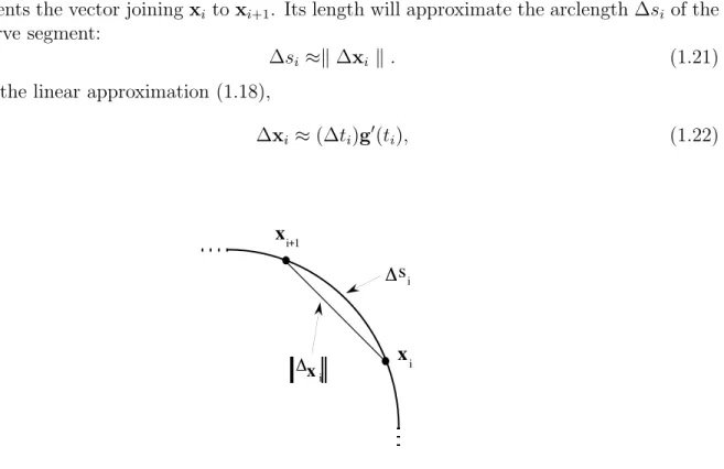
defines N + 1 points on the curve (1.20), given by xi = g(ti), i = 0,1, . . . , N. Joining

these points in order with straight lines yields a polygonal arc that can be regarded as approximating the curve C. See Figure 1.13 for the caseN = 4.

x0 x1 x2 x3 x4 C

(2)

The ith _increment

∆xi =xi₊₁−xi

represents the vector joiningxi toxi+1. Its length will approximate the arclength ∆si of the

ith curve segment:

∆si ≈k∆xi k. (1.21)

Using the linear approximation (1.18),

∆xi ≈(∆ti)g′(ti), (1.22) xi !si xi+1 !_x i

Figure 1.14: The length of the line segment approximates the arclength of the curve segment.

where

∆ti =ti₊₁−ti,

for ∆ti sufficiently small.

It follows from (1.21) and (1.22) that

∆si ≈kg′(ti)k∆ti, i= 0,1, . . . N −1, (1.23)

for ∆ti sufficiently small. Summing over N curve segments gives an approximation for the

total arclength s: s≈ N₋₁ X i₌₀ kg′₍_t i)k∆ti.

The sum is a Riemann sum for the integral

Z b

a

(3)

and will thus approximate the integral with increasing accuracy as the partition becomes increasingly fine. We thus expect that the arclength s of the curve x = g(t), a ≤ t ≤ b is given by s= Z b a kg′₍_t₎_k_dt. _(1.24) Comments:

i) In practice we use equation (1.24) as the definition of arclength of a C1 _{curve. The} steps leading to (1.21) do not constitute a proof because of the approximations made, but should be viewed as a heuristic justification of (1.24). It is important to understand these steps, however, because they form the basis for the definition of the concept of line integral in Chapter 2.

ii) If the curveC represents the path of a particle then the integrand kg′₍_t₎_k _{in (1.24) is}

the speed of the particle, and so the formula (1.24) has a simple physical interpretation: distance travelled is the integral of the

speed with respect to time.

1.2 Vector fields

So far we have considered vector-valued functionsg: [a, b]→Rn

, which define curves. In this section we consider a second type of vector-valued function of great importance in physics and engineering applications, namely vector fields.

1.2.1 Examples from physics

Many physical quantities are characterized by giving a magnitude, i.e. a real number, at each point of space. Such quantities are represented by real-valued functions f : R3 _→ _R_. Functions of this type, when used in a physical context, are called scalar fields. Some examples are the following:

- the temperature T(x, y, z) at a point of a body, - the pressure p(x, y, z) at a point of a fluid,

- the electric charge density σ(x, y, z) on the surface of a metallic object, - the intensity of light I(x, y, z) falling on an object,

. . .and so on.

On the other hand there are many physical quantities that are characterized by giving a magnitude and a direction, i.e. a vector, at each point of space. Such quantities are represented by a function F : _R3 _→

(4)

unique vector F(x, y, z) ∈ _R3_{. Functions of this type, when used in a physical context, are} called vector fields.

Example 1.7:

The gravitational field due to a spherical body of mass M, such as the earth, can be represented by the vector field Fdefined by

F(x, y, z) =−GM

r3 r, (1.25)

where r= (x, y, z), r=krk=px2₊_y2 ₊_z2_{, and} _G _{is the gravitational constant.}

The vector F(x, y, z) represents the force exerted on a test body of unit mass placed at position (x, y, z). The minus sign accounts for the fact that the test body will be attracted to the earth, i.e. F(x, y, z) points towards the origin.

x z y F(x ,y, z) r=( x , y, z)

Figure 1.15: The gravitational field of a spherical body.

Comment:

In this example the domain of the vector field is the open set U =R3_{− {}₍₀_,₀_,₀₎_}_.

Example 1.8:

Consider a distribution of fluid flowing in a steady state. Then at a given point (x, y, z) the fluid has a uniquely defined velocity v(x, y, z) that is independent of the time. The vector field v is called thevelocity field of the fluid. See Figure 1.16.

Example 1.9:

There is also a scalar field ρ(x, y, z) associated with a fluid, namely the mass density of the fluid, which is independent of time for a steady state flow. One is interested in the rate at which mass is transferred by the fluid, and this rate is determined by another vector field formed fromρ and v, as follows.

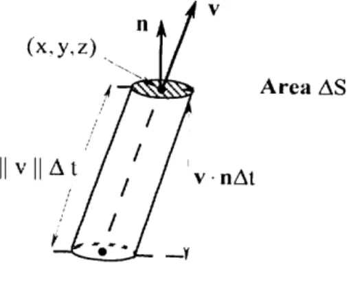
Consider a plane surface element of area ∆S, with unit normal vector n, located at position (x, y, z). In time ∆t, the fluid in a column of length kvk∆t will flow through the surface element. Since the vertical height of the column is v···n∆t (see Figure 1.17) the volume of the column, and hence the volume of fluid transported, is

(5)

(x , y,z )

v( x ,y ,z )

Figure 1.16: The velocity field of a fluid.

Figure 1.17: Flow of a fluid through a plane surface element.

It follows that mass of fluid transported across the surface element in time ∆t is ∆M ≈ρ∆V ≈ρv·n∆S∆t.

Thus, the mass transferred per unit time across the surface element is

(ρv)···n∆S. (1.26)

This quantity is called the mass flux across the surface element: “flux” means “rate of flow”.

It is worth checking the physical dimensions of the mass flux (note that n, being a unit normal, is dimensionless):

[(ρv)···n∆S] = (M L−3₎₍_LT−1₎₍_L2_{) =} _{M T}−1_, i.e. mass per unit time.

(6)

The mass flux (1.26) is determined by the vector field J defined by

J(x, y, z) = ρ(x, y, z)v(x, y, z), (1.27) which has physical dimensions

[ J ] =M T−1_L−2_,

i.e. mass per unit time per unit area. This vector field, which describes the transport of mass by the fluid, is called the mass flux density of the fluid.

Comment:

In (1.26) and the preceding equations, ρ and v are evaluated at the given point (x, y, z). We are assuming that kvk∆t and ∆S are sufficiently small thatρ and vcan be regarded as constant throughout the cylinder in Figure 1.17.

Example 1.10:

Any C1 _{scalar field} _u_in _R3 _{determines a vector field} _F _in_R3 _{according to}

F(x, y, z) =∇u(x, y, z), (1.28) where ∇u is thegradient of the scalar field, defined by

∇u= ∂u ∂x, ∂u ∂y, ∂u ∂z . (1.29)

In other words, the gradient of a C1 _{scalar field is a vector field. This type of vector field} will arise frequently in the course.

The concept of a flux density vector field, as in Example 1.3, where we studied the mass flux density, applies to any physical quantity that is transferred in space, e.g. heat energy, which is the next example.

Example 1.11:

Consider a piece of material that is heated on one side and cooled on the other in such a way that the temperature attains a steady state, i.e. the temperature u(x, y, z) depends on position (x, y, z) but not on time t. The temperature is a scalar field. From everyday experience we know that heat will flow (i.e. energy will be transferred) from hot regions to cold regions. As with mass flow, heat flow can be described mathematically by a vector field

j(x, y, z), which gives the rate of heat transfer through a small surface element at (x, y, z), called the heat flux density, i.e.

(j·n)∆S

is the rate of transfer of heat through a small plane surface element of area ∆S and having unit normal n (compare with equation (1.26)).

Experimental work shows that the heat flux density may be represented byFourier’s law

(7)

wherek > 0 is a constant. This law is plausible physically, since one expects that the larger is the spatial temperature gradient, represented by the gradient∇u, the larger will be the rate of heat transfer. The constant k, called the thermal conductivity, depends on the material, being bigger for a good conductor of heat than for a poor conductor (e.g. kcopper/kglass ≫1).

Having given some physical examples of vector fields we now introduce the terminology formally.

Let U be an open subset of Rn

. A vector field on U is a function F : U → Rn

, whose domain isU and whose range is inRn, i.e. Fassigns to eachx∈ U a unique vectorF(x)∈Rn. The vector fields we work with will usually be of class C1_{, which means that the} _n component functions,

F(x) = (F1(x), . . . , Fn(x))

are C1 _functions.

We shall also assume that the domain U is a connected set, which means that U is not the union of two or more disjoint sets.

1.2.2 Field lines of a vector field

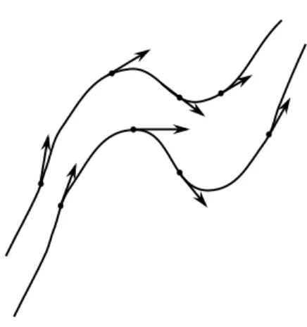
One visualizes a vector fieldFon an open set U ⊂R3 as a “field of vectors”, represented by arrows, attached to the points of U. Thelength of the vector at a point gives thestrength of the fieldat the point, and the arrow gives the direction of the field.

It is also helpful to think of the family of curves in U with the property that at each point

P the tangent to the curve throughP equals the vector field evaluated atP. These curves are called thefield lines1 _{of the vector field. One thinks of a field line threading its way through} the vector field, always following the direction of the vector field (see Figure 1.18).

Figure 1.18: Two field lines of a vector field.