i
Ensemble Learning with GSGP
Olivier GAU
Dissertation presented as partial requirement for
obtaining the Master’s degree in Advanced Analytics
ii
NOVA Information Management School
Instituto Superior de Estatística e Gestão de Informação
Universidade Nova de LisboaENSEMBLE LEARNING WITH GSGP
por
Olivier GAU
Dissertação apresentada como requisito parcial para a obtenção do grau de Mestre em Métodos Analíticos Avançados
Orientador: Leonardo Vanneschi
Ac k n o w l e d g e m e n t s
I would like to thank Professor Leonardo Vanneschi, Professor Mauro Castelli and Assistant Professor Illya Bakurov for their guidance and help during this project.
A b s t r a c t
The purpose of this thesis is to conduct comparative research between Genetic Pro-gramming (GP) and Geometric Semantic Genetic ProPro-gramming (GSGP), with diff er-ent initialization (RHH and EDDA) and selection (Tournamer-ent and Epsilon-Lexicase) strategies, in the context of a model-ensemble in order to solve regression optimization problems.
A model-ensemble is a combination of base learners used in different ways to solve a problem. The most common ensemble is the mean, where the base learners are com-bined in a linear fashion, all having the same weights. However, more sophisticated ensembles can be inferred, providing higher generalization ability.
GSGP is a variant of GP using different genetic operators. No previous research has been conducted to see if GSGP can perform better than GP in model-ensemble learning. The evolutionary process of GP and GSGP should allow us to learn about the strength of each of those base models to provide a more accurate and robust solution. The base-models used for this analysis were Linear Regression, Random Forest, Support Vector Machine and Multi-Layer Perceptron. This analysis has been conducted using 7 different optimization problems and 4 real-world datasets. The results obtained with GSGP are statistically significantly better than GP for most cases.
Keywords: GP, GSGP, Model-ensemble, Linear Regression, Random Forest, Support Vector Machine, Multi-Layer Perceptron
R e s u m o
O objetivo desta tese é realizar pesquisas comparativas entre Programação Genética (GP) e Programação Genética Semântica Geométrica (GSGP), com diferentes estraté-gias de inicialização (RHH e EDDA) e seleção (Tournament e Epsilon-Lexicase), no contexto de um conjunto de modelos, a fim de resolver problemas de otimização de regressão.
Um conjunto de modelos é uma combinação de alunos de base usados de diferentes maneiras para resolver um problema. O conjunto mais comum é a média, na qual os alunos da base são combinados de maneira linear, todos com os mesmos pesos. No entanto, conjuntos mais sofisticados podem ser inferidos, proporcionando maior capacidade de generalização.
O GSGP é uma variante do GP usando diferentes operadores genéticos. Nenhuma pesquisa anterior foi realizada para verificar se o GSGP pode ter um desempenho melhor que o GP no aprendizado de modelos. O processo evolutivo do GP e GSGP deve permitir-nos aprender sobre a força de cada um desses modelos de base para fornecer uma solução mais precisa e robusta. Os modelos de base utilizados para esta análise foram: Regressão Linear, Floresta Aleatória, Máquina de Vetor de Suporte e Perceptron de Camadas Múltiplas. Essa análise foi realizada usando 7 problemas de otimização diferentes e 4 conjuntos de dados do mundo real. Os resultados obtidos com o GSGP são estatisticamente significativamente melhores que o GP na maioria dos casos.
Palavras-chave: GP, GSGP, Model-ensemble, Linear Regression, Random Forest, Sup-port Vector Machine, Multi-Layer Perceptron
C o n t e n t s
List of Figures xv
List of Tables xvii
Listings xix Acronyms xxi 1 Introduction 1 2 Theory 3 2.1 Machine Learning . . . 3 2.2 Ensemble Learning . . . 4 2.2.1 Stacked Generalization . . . 5 2.3 Regression Estimators . . . 5
2.3.1 Multiple Linear Regression . . . 6
2.3.2 Random Forest Regression . . . 6
2.3.3 Support Vector Machine Regression . . . 7
2.3.4 Multilayer Perceptron Regression . . . 7
2.4 Evolutionary Algorithm. . . 8
2.4.1 Genetic Programming . . . 8
2.4.2 Geometric Semantic Genetic Programming . . . 10
2.4.3 Initialization . . . 11
2.4.4 Parent Selection . . . 15
2.4.5 Fitness Evaluation . . . 16
2.4.6 Elitism . . . 16
2.4.7 Semantic Stopping Criterion . . . 17
2.4.8 Genetic Programming as a Meta-Learning Technique. . . 18
3 Methodology 21 3.1 Proposed approach . . . 21
3.2 Objectives . . . 21
3.3 Ensemble hyper-parameters . . . 22
C O N T E N T S
3.5 Problem dataset - Train and Test split . . . 25
3.6 Base Learners hyper-parameters tuning. . . 26
3.7 Base Learners dataset - K-Fold data generation . . . 26
3.8 Base Learners dataset - Train and Validation split . . . 27
3.9 Function set and Terminal set . . . 29
3.9.1 Decision . . . 29 3.10 Fitness Evaluation . . . 30 3.10.1 Memoization. . . 30 3.11 Parent Selection . . . 31 3.11.1 Tournament . . . 31 3.11.2 Epsilon Lexicase . . . 31 3.12 Stopping Criteria . . . 31 4 Results 33 4.1 Performance Analysis . . . 33 4.2 Statistical Assessment . . . 35
4.2.1 Comparison of system’s hyper-parameters - Global . . . 35
4.2.2 Comparison of system’s hyper-parameters - By algorithm and BLs tuning . . . 36
4.2.3 Best S-GSGP vs Best S-SGP - By problem type and base learners hyper-parameters . . . 39
4.2.4 Comparison of the best performing system vs BLs . . . 40
5 Discussion 43 5.1 Summary . . . 43 5.2 Interpretation . . . 44 5.3 Implications . . . 45 5.4 Limitations . . . 45 5.5 Recommendations . . . 45 6 Conclusion 47 Bibliography 49
A Appendix - Ensemble Workflow 55
B Appendix - Performance by dataset 57
C Appendix - Boxplots and Learning curves 61
D Appendix - Tuned Base Learners Hyper-parameters 65
C O N T E N T S
II Annex - Best ensemble solution’s string 73
II.1 Branin - Solution’s string . . . 73
II.2 Discus - Solution’s string . . . 73
II.3 Griewank - Solution’s string . . . 74
II.4 Kotanchek - Solution’s string . . . 74
II.5 Mexican Hat - Solution’s string. . . 74
II.6 Rastrigin - Solution’s string . . . 75
L i s t o f F i g u r e s
2.1 Example of a Stacked Generalization consisting of 1 layer of five
base-learners. . . 6
2.2 Evolutionary Algorithm. . . 8
2.3 Pseudo-code for a simple version of Evolutionary algorithm. . . 9
2.4 Pseudo-code for a simple version of Genetic Programming algorithm. . . 9
2.5 Example of a tree-based representation of a GP individual . . . 10
2.6 Pseudo-code for Ramped Half-and-Half initialization method. . . 12
2.7 Example of functioning of RHH for a population of size 6 and maximum depth of 3. . . 13
2.8 Pseudo-code of EDDAm−n% system, in which demes are left to evolve formgenerations. . . 14
2.9 Pseudo-code for Lexicase Selection (LS) technique. . . 15
2.10 Illustration of SSC’s functioning. Thestarin the figure represents the target vector on training data. . . 18
3.1 Optimization Problems . . . 25
3.2 Dataset split representation . . . 26
3.3 Base Learners dataset generation . . . 28
3.4 Base Learners predictions data split . . . 28
3.5 Decision . . . 29
A.1 Ensemble Workflow . . . 56
C.1 Branin - BLs not tuned - Boxplots and Learning curves . . . 61
C.2 Parkinson - BLs not tuned - Boxplots and Learning curves . . . 62
C.3 Weierstrass - BLs not tuned - Boxplots and Learning curves . . . 62
C.4 Boston - BLs tuned - Boxplots and Learning curves . . . 63
C.5 Ppb - BLs tuned - Boxplots and Learning curves . . . 63
C.6 Parkinson - BLs tuned - Boxplots and Learning curves . . . 64
I.1 Branin - S-GSGP and Base Learners 3D Graphs . . . 69
I.2 Discus - S-GSGP and Base Learners 3D Graphs . . . 70
L i s t o f F i g u r e s
I.4 Kotanchek - S-GSGP and Base Learners 3D Graphs . . . 71
I.5 Mexican Hat - S-GSGP and Base Learners 3D Graphs . . . 71
I.6 Rastrigin - S-GSGP and Base Learners 3D Graphs . . . 72
L i s t o f Ta b l e s
3.1 Enumeration of hyper-parameters. It is worth to notice thatdecisionstands for the decision expression operator proposed in [20],BLs pre-training indi-cates if the BLs were tuned or not,-LSrepresents the selection algorithm proposed in [36],P(C) andP(M) indicate the crossover and mutation prob-abilities, andvalidation fitnessstands for the stopping criteria which oper-ates upon the fitness calculated from validation partition by estimating the point from where further induction allows further generalization. . . 23
3.2 Mathematical formulation of synthetic regression problems used in this study. The problems are listed in alphabetical order. . . 24
3.3 Enumeration of search space’s boundaries (the domain) for each function. It is worth to notice that columnsLower andUpper stand for lower and upper bounds of two dimensional search space. . . 24
3.4 Description of real-world regression problems used in the experiments. For each problem, the name (ID), number of input features (#Features), data instances (#Instances) and field of application (Field) is presented. . . 25
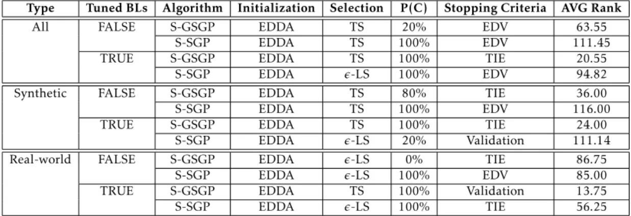
4.1 Average performance rank - Top 5 by problem type. . . 34
4.2 Average performance rank - Best system by problem type, base learners hyper-parameters and algorithm. . . 34
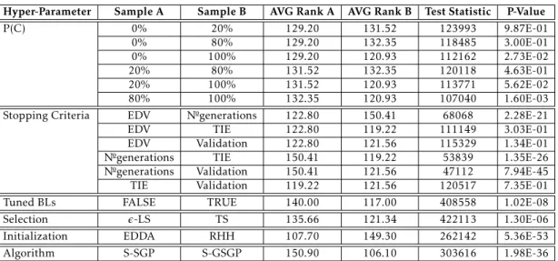
4.3 Statistical assessment - Global . . . 35
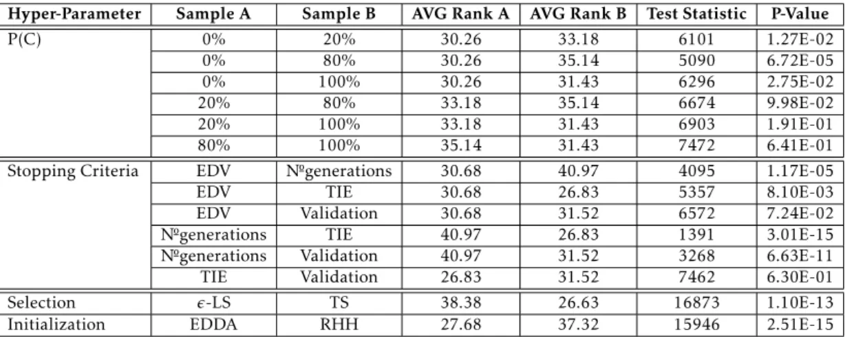
4.4 Statistical assessment - Without tuned BLs, for all S-GSGP, by hyper-parameter 36
4.5 Statistical assessment - Without tuned BLs, for all S-SGP, by hyper-parameter 37
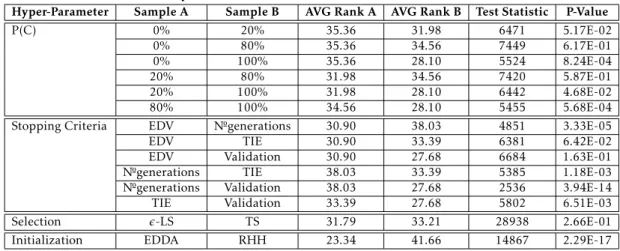
4.6 Statistical assessment - With tuned BLs, for all S-GSGP, by hyper-parameter 38
4.7 Statistical assessment - With tuned BLs, for all S-SGP, by hyper-parameter 39
4.8 Statistical assessment - Comparison of best S-GSGP vs best S-SGP - By problem type and base learners hyper-parameters. . . 39
4.9 Statistical assessment - Best performing ensemble system for all problems and BLs: [Tuned BLs, S-GSGP, EDDA, TS, P(C) 100%] - (Average RMSE by problem in table B.3) . . . 41
B.1 Avg RMSE - Top 5 - Synthetic datasets . . . 58
L i s t o f T a b l e s
B.3 Avg RMSE - Best performing ensemble system for all problems and BLs: [Tuned BLs, S-GSGP, EDDA, TS, P(C) 100%] . . . 59
D.1 Random Forest Regression - Tuned Hyper-parameters by problem . . . . 65
D.2 Support Vector Regressor - Synthetic Problems - Tuned Hyper-parameters by problem . . . 66
D.3 Linear Support Vector Regressor - Real-world Problems - Tuned Hyper-parameters by problem . . . 66
D.4 Multi-layer Perceptron Regressor - Tuned Hyper-parameters by problem 66
L i s t i n g s
3.1 Python code for Train and Test split . . . 25
3.2 Base Learners Train and Predict pseudo code . . . 27
3.3 Function set variable . . . 29
3.4 Memoization Pseudo-code . . . 30
Ac r o n y m s
ATA Automatic Threshold Adaptation. BL Base Learner.
EDV Error Deviation Variation.
EDV-SCC Error Deviation Variation Semantic Stopping. GP Standard Genetic Programming.
GSC Geometric Semantic Crossover.
GSGP Geometric Semantic Genetic Programming. GSM Geometric Semantic Mutation.
GSO Geometric Semantic Operators. LS Lexicase Selection.
not tuned BLs Base Learners whose hyper-parameters were not estimated, instead kept default.
SC Stopping Criteria. S-GSGP Stacking with GSGP. S-SGP Stacking with standard GP.
AC R O N Y M S
S-GP Stacking with GP-like techniques (any). TIE Training Improvement Effectiveness.
TIE-SCC Training Improvement Effectiveness Semantic Stopping.
TS Tournament Selection.
tuned BLs Base Learners whose hyper-parameters were estimated from Grid-Search Cross Validation.
C
h
a
p
t
e
r
1
I n t r o d u c t i o n
Ensemble Learning (EL) is a sub-field in Machine Learning which is inspired on hu-mans’ natural tendency to seek and weight the opinion of others’ before making any important decision. Under this perspective, EL consists of combining several individ-ual models, the base-learners, in a way to produce a model (the ensemble), which is expected to solve a given task better than any of the base-learners [43]. Stacked Gen-eralization, or simply stacking, consists of training an ensemble from the combined predictions of several other, ideally heterogeneous, base-learners. More specifically, it consists of training the base-learners to solve the underlying task, then it trains a meta-learner from their predictions [55].
In this paper, we study Genetic Programming (GP) as the meta-learner which combines four heterogeneous base-learners. More technically, we allow GP to automat-ically evolve computer programs having as a terminal set the combined predictions of four heterogeneous base-learners. The objective which drives such an evolutionary process is ensemble’s generalization ability on a given Supervised Machine Learning (SML) task. For the sake of simplicity, we will refer to this kind of approaches as Stacking-GP (S-GP). Our motivation relies upon intrinsic properties of GP. We expect that, withproperlychosen operators and hyper-parameters, GP is capable of combining base-learners in a highly non-linear fashion which could better exploit their outputs and achieve superior generalization ability.
In fact, the usage of S-GP is not new in the research-field. To our knowledge, the first work dates to 2006 [26] where GP was used to combine ten Artificial Neural Networks into an ensemble. Since then, several other important contributions were proposed [1,12,20,29]. Nevertheless, we consider that research in S-GP is still much in demand and we have identified two major reasons for that. First, we have found that the majority of contributions in S-GP are assessed on classification problems, whereas
C H A P T E R 1 . I N T R O D U C T I O N
none of the previous works provides a concise benchmark over regression problems. The second reason has to do with the recent methodological achievements of the in the research field: Geometric-Semantic Operators (GSO), Semantic Stopping Criterion (SSC), -Lexicase Selection (-LS) and Evolutionary Demes Despeciation Algorithm (EDDA) are among numerous recent methods which were not broadly studied in the context of S-GP. In the objective of this paper consists of covering aforementioned gaps by providing a concise overview of S-GP over 7 synthetic and 4 real-world regression problems while using state-of-the art achievements in the field of GP.
This thesis is organized as follows: in Chapter2we introduce the necessary the-oretical background. Chapter3describes the research hypothesis and the proposed approach. Chapter4presents our experimental framework, results’ exhibition, their detailed analysis. A critical discussion is made in Chapter5. Finally, Chapter6 con-cludes the work and proposes ideas for future research.
C
h
a
p
t
e
r
2
T h e o r y
2.1
Machine Learning
Machine Learning (ML) is a field of artificial intelligence using algorithms and com-putation power to learn patterns from a given sample of observations called a dataset, without human interaction. An algorithm is a function composed of sets of rules in charge of the learning process using a dataset as input data.
The data can be provided in a tabular form composed of instances and features, corresponding respectively to the rows and columns in a worksheet. This structure can contain an expected value (target) for each set instance (sample) of the dataset. To transform data (sample and target) into knowledge, recognizable elements have to be detected in order to give a prediction for an unseen instance.
If there is no target value the analysis of the data will be unsupervised (e.g. cluster-ing, dimension reduction, and association).
If there is a target the algorithm can adjust its set of rules to by learning from the comparison of the result to the target then we talking about supervised learning. When the target value is a category or numerical, the algorithm’s task will be a classification for the former or regression for the latter. In this thesis, we will focus on regression.
C H A P T E R 2 . T H E O RY
2.2
Ensemble Learning
In the field of Machine Learning, one can find numerous methodologies which mimic biological and social processes of the real world. The Artificial Neural Network (ANN), for example, is a biologically-inspired computer system which simulates the Biological Neural Network (BNN) and its bio-chemical processes [25]. As a result, an ANN con-sists of a set of interconnected layers of neurons (the basic processing units) which, all together, form a powerful and versatile computer system able to solve numerous com-plex optimization problems such as automatic speech and image recognition, natural language processing, bio-informatics, fraud-detection, etc [46]. The Particle Swarm Optimization (PSO) [19] is another type of biological system - a social system - whose computational metaphor is the collective behavior of simple individuals interacting with their environment and each other, like a flock of birds or schools of fishes. The individual in this algorithm is a particle, which is described by its position and veloc-ity in the search space. The direction in which each particle moves is influenced by the behaviour of the other particles in the swarm - the social factor - and individual memory - the cognitive factor. Such computer system is frequently used in function optimization, ANNs training, fuzzy system control and other areas.
Ensemble Learning (EL), in this context, is not an exception as it reflects the nat-ural predisposition of human beings to seek for other opinions before making any important decision. We tend to weigh several individual opinions, and combine them through some thought process in order to reach a final decision, which is expected to be the most appropriate [43]. In this sense, an ensemble combines several indi-vidual models, the base-learners (BLs), in a way which yields a model whose overall generalization ability is expected to bebetterwhen compared to any of its BLs. In fact, there is a considerable number of empirical studies showing that in both classification and regression problems the ensembles are significantlysuperiorthan the BLs which compose them [7,10,11,18,21,55], and several theoretical explanations have been proposed to justify their superiority [55], majority of them based on the so called bias-variance decomposition of the error. Apart from that, when provided a spectrum of SML techniques, it is true that the most appropriate is frequently chosen based on some global approximation measure such as the Root Mean Squared Error (RMSE). Con-sidering a SML problem and two candidate modelling techniques,aandb, it might happen thata, from the perspective of some global performance measure, provides
betterglobal approximation on a given problem thanb, howeverbmight exhibitbetter
local approximation thana, i.e., might approximate better thanain a specific region of the search space. In this context, by wisely using bothaandbin an ensemble, one can combine the most well-approximated regions of the search space allowing for levels of global approximation which aresuperiorto those provided byaandbwhen taken singularly. Another relevant motivation for using ensembles is the difficulty the one
2 . 3 . R E G R E S S I O N E S T I M AT O R S
faces when choosing the most appropriate modeling technique when solving a given problem. In fact, the abundance of conceptually distinct SML techniques, along with a varied number of adjustable parameters they bring, makes the SML takslaboriousand
time-consuming. Under this perspective, using an ensemble can substantially reduce thiscomplexityto a limited set of models and/or parameters.
2.2.1 Stacked Generalization
The field of EL, although relatively recent, has been extensively researched and several conceptually different approaches, along with different ways to categorize them, were proposed so far. In general terms, Ensemble Methods (EMs) differ in the way input data is represented and manipulated within the system, the procedure to make the final prediction, whether ensemble’s BLs can be trained independently from each other, etc. [43,45,56].
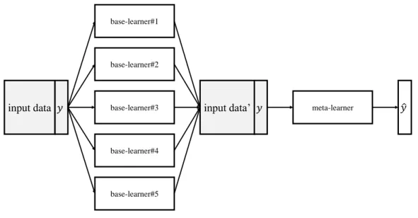
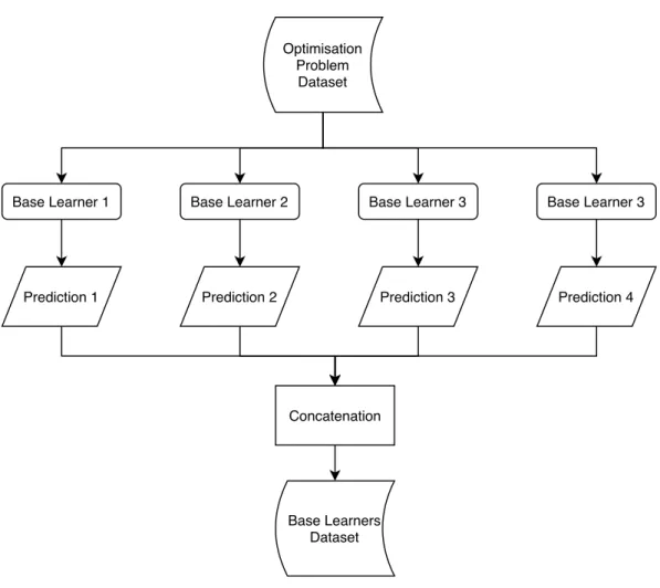
In this sub-sub-section we will provide an overview of stacked generalization, pro-posed by David H. Wolpert [55] in 1992, because the approach we propose in this paper strongly relates to this specific ensemble method. Stacked generalization, or simplystacking, consists of training a meta-learner from the combined predictions of two (or more) BLs. In other words, the predictions obtained from the BLs, which are trained independently from each other, are used as inputs of a meta-learner which can be any known ML technique. In practice, the system can have several sequential layers of BLs before using one final meta-learner. In figure2.1you can find a visual representation of stacking consisting of one layer of five BLs.
The approach we present in this paper has a simple although rational motivation -in the context of stack-ing, to use GP as the meta-learner from comb-ined predictions of several conceptually different BLs.
2.3
Regression Estimators
In statistics, one or many independent variables also known as features are used to describe one dependent variable also known as a target. Regression estimators are statistical methods (algorithms) which allow us to model either a linear or a non linear relationship between independent and dependent variables.
In a linear relationship, the proportion between the dependent and independent variables will remain the same, the plot resulting in a flat line. In a nonlinear relation-ship, the logic between the dependent and independent variable is unstable, the plot resulting in a curve.
C H A P T E R 2 . T H E O RY input data base-learner#2 base-learner#3 base-learner#4 base-learner#1 base-learner#5 meta-learner 𝑦ො 𝑦 input data’ 𝑦
Figure 2.1: Example of a Stacked Generalization consisting of 1 layer of five base-learners.
2.3.1 Multiple Linear Regression
In supervised machine learning, singular linear regression is a popular method to find the relationship between one independent variable (the feature) and one dependent variable (the target). This relationship between variables can be represented by the equation Y = a + b X with Y the dependent variable and X the independent variable. The result of this analysis is a predictive model fitting the observed features and corre-sponding target.
Multiple linear regression works similarly but is using several independent vari-ables, attributing a slope coefficient to each of them, determining the effect each of them will have on the dependent variable.
2.3.2 Random Forest Regression
Decision Tree is a predictive model that can be use for classification and regression. The model uses a tree-like structure composed of decision nodes, branches and leaf nodes. The decision nodes represent tests with different possibilities represented by branches. A branch can be followed by a decision node or a leaf node. The leaf node corresponds to the final outcome. The solution allows to understand visually the different predictions of the model following a clear logic (tests -> possibilities -> outcomes) based on the given dataset.
2 . 3 . R E G R E S S I O N E S T I M AT O R S
The random forest model is a type of additive model that makes predictions by combining decisions from a sequence of base learners. More formally we can write this class of models as: g(x)=f0(x)+f1(x)+f2(x)+... where the final model g is the sum of simple base learners. Here, each base learner is a simple decision tree. This broad tech-nique of using multiple models to obtain better predictive performance is called model ensembling. In random forests, all the base learners are constructed independently using a different sub-sample of data.
A Random Forest is an ensemble technique capable of performing both regression and classification tasks with the use of multiple decision trees and a technique called Bootstrap Aggregation, commonly known as bagging. In the Random Forest method, Bagging involves training each decision tree on different data samples (sampling with replacement).
2.3.3 Support Vector Machine Regression
Support Vector Machine (SVM) [9] is an algorithm mainly used for classification pur-poses where provides good accuracy with less computational power. The goal of SVM for classification is to find the hyperplane in an n-dimensional space able to separate classes with the widest margin possible. The support vectors are data points located at the border of the margin.
SVM can also be used for regression problems, but in this case, it will produce hy-perplanes in n-dimensional space whereas many data points can fit within the margin of tolerance ‘epsilon’. Only the data points outside the margin ’epsilon’ will be used to calculate the error (distance from the border of the margin ’epsilon’). The hyperplane with the lowest error will be selected.
2.3.4 Multilayer Perceptron Regression
An Artificial Neural Network (ANN) is an algorithm mimicking the structure of the human brain. It is composed of connected artificial neurons, also known as nodes, which are mathematical functions similar to biological neurons in their process. A node can have multiple inputs and outputs as a result of its operation.
A Multi-Layer Perceptron (MLP) is the first and most simple of feedforward type of ANN, its structure consisting of at least three layers of nodes.
An input layer is in charge of carrying the original data to the network. One or more hidden layers placed between the input and output layer are computing the weights attributed to each node in the network. Finally, the output layer, which is the final layer of the network is producing the output result. Except for the input nodes,
C H A P T E R 2 . T H E O RY Initialization Selection Termination Mutation Crossover
Figure 2.2: Evolutionary Algorithm
each node uses a nonlinear activation function that is able to solve complex problems, taking a node’s output as input and outputting its interpretation.
2.4
Evolutionary Algorithm
This particular branch of data science relies heavily on the biological principles gov-erning the natural world. In a nutshell, deoxyribonucleic acid or DNA for short is a molecule containing the genetic code of all organisms on Earth. Each cell in each organism contains these bespoke instructions for which proteins should be made by which cell. It’s the reason why parents and children share certain physical traits. The passing of the genes is called heredity and a gene is its basic unit. Humans are a unique blend of their parent’s genetic material which is joined through the process of recom-bination after a reproductive event. A mutation is what we call a change occurring in our DNA sequence due to internal (e.g. DNA copying fault) or external (e.g. UV light, cigarettes) factors without reproduction. In biology, natural selection means that certain human traits/genes are preferable to others and evolution is more likely to preserve them in our genetic material over generations to ensure survival by picking the parents with the most beneficial features for reproduction.
In data science however, Evolutionary Algorithm (Figures 2.2 and2.3) is a sub-set of evolutionary computation, based on population and optimization, inspired by biology or more specifically it’s sub-field of genetics. By mimicking processes such as reproduction, mutation, recombination, and selection it is able to find a solution within given limitations. The process follows this pseudo code, the steps of which we will discuss later on.
2.4.1 Genetic Programming
In the field of Evolutionary Algorithms (EAs), Genetic Programming (GP) is among the most recent and dynamically growing sub-fields. Introduced and popularized by
2 . 4 . E V O LU T I O N A RY A L G O R I T H M
1. Create Initial population;
2. Calculate Fitness of all individuals; 3. While Termination condition not met:
a) Select fitter individuals for reproduction; b) Recombine between individuals;
c) Mutate individuals;
d) Evaluate fitness of all individuals; e) Generate a new population; 4. Return Best individual;
Figure 2.3: Pseudo-code for a simple version of Evolutionary algorithm.
John Koza [30–34], GP is, in fact, an adaption of Genetic Algorithm (GA) for evolution of computer programs. In simple terms, GP is a population-based algorithm which follows principles ofDarwin’s Theory of Evolution[17] to evolve computer programs, among the space of all possible computer programs, which can solve a given opti-mization problem. The figure2.4contains the simple version of the pseudo-code of GP:
1. generate an initial populationP ofN individuals by means of an initialization method; 2. repeatuntil satisfying some termination condition:
a) evaluate the fitness∀i∈P; b) create empty populationP0 ;
c) repeatuntilP containsnindividuals:
i. choose a genetic operator: crossover or mutation with probabilitypcor 1−pm,
respectively;
ii. by means of a selection method, select two individuals fromP if crossover was chosen, otherwise select one;
iii. apply the variation operator chosen in point 2.3.1 to the individual(s) selected in point 2.3.2;
iv. insert the individual(s) obtained in point 2.3.3 intoP0; d) replaceP withP0
; 3. return the best individual
Figure 2.4: Pseudo-code for a simple version of Genetic Programming algorithm. As we can see from2.4, evolution of the population starts with individuals’ initial-ization. Then, by applying selection mechanism and variation operators to the selected
parents,offspringare created and transited to the next generation. This process iterates until reaching certain stopping criteria (like the maximum number of generations).
C H A P T E R 2 . T H E O RY
given programming language arranged in a particular way. Commonly, individuals are represented in a tree-based structure. For the sake of example, consider the fol-lowing two sets of program elements, necessary components of a computer program:
terminals={x1, x2, x3}andf unctions={+, −, ∗, / }. A possible individual resulting
from composition of such elements is represented in figure2.5.
Figure 2.5: Example of a tree-based representation of a GP individual
In other words, an individual evolved by means of GP can be a mathematical function of the formf(x1, x2, x3) =X1∗X1+X2−X3.
2.4.2 Geometric Semantic Genetic Programming
In the terminology adopted by a considerable part of Genetic Programming (GP) re-search community [8,27,28,35,39], the termsemanticsdefines the vector of output values of a candidate solution, calculated on the training observations. Following this definition, a candidate solution obtained by means of GP can be seen as a point in multidimensional space of dimensionality number of observations in the training set. Let’s call itsemantic space.
Geometric Semantic Genetic Programming (GSGP) is a recently introduced variant of GP where standard crossover and mutation operators are replaced by the so-called
Geometric Semantic Operators(GSOs) [38]. GSOs, gained popularity in the GP commu-nity [13, 15,16,50–53] because of their geometric property of inducing a unimodal error surface (characterized by the absence of locally optimal solutions) for any Super-vised Machine Learning (SML) problem. The proof of this property can be found in [38,
50]. In this document, we report the definition of the GSOs, as given by Moraglio et al. for real functions domains, since these are the operators that we have used in our experiments. For applications that consider other types of data, the reader is referred to [38] and [3].
Geometric Semantic Crossover(GSC) generates, as the unique offspring of parents
T1, T2:Rn→R, the expression: TXO= (T1·TR) + ((1−TR)·T2), where TR is a random
real function whose output values range in the interval [0,1]. Moraglio and co-authors show that GSC corresponds to geometric crossover in the semantic space, i.e., the point representing the offspring stands on the segment joining the points representing the
2 . 4 . E V O LU T I O N A RY A L G O R I T H M
parents. Consequently, the GSC inherits the key property of geometric crossover: the offspring is never worse than the worst of the parents.
Geometric Semantic Mutation (GSM) returns, as the result of the mutation of an individual T :Rn→R, the expression: TM=T+ms·(TR1−TR2), where TR1 andTR2
are random real functions with codomain in [0,1] andmsis a parameter called the mutation step. Similarly to GSC, Moraglio and co-authors show that GSM corresponds to the box mutation on semantic space. Consequently, the operator induces a unimodal error surface on any SML problem.
As Moraglio and co-authors point out, GSOs create an offspring which is substan-tially larger than their parents, and the fast growth of the individuals’ size rapidly makes fitness evaluation very slow, making the system unusable. As a solution to this problem, Castelli et al. [13] proposed a computationally efficient implementation of Moraglio’s operators making them usable in practice.
Given fact GSC generates an offspring whose semantics stands on the segment joining the semantics of the two parents, it can only achieve the global optimum if the semantics of the individuals in the population “surround” the semantics of the global optimum. Using the terminology of [14,41], GSC only has the possibility of generating a globally optimal solution if it lays within the semanticconvex hullidentified by the population. The need for overcoming this drawback has led to several methods to properly initialize a population of GSGP, like for instance the ones presented in [2,40,
54].
2.4.3 Initialization
In any Evolutionary Algorithm (EA), population initialization is the very first step in the evolutionary process [17]. Assuming a tree-based representation, the initialization of individuals in GP consists of creating almost random trees, such that program elements, starting from the root node of the tree, are combined one after another in a specific manner, until reaching a pre-defined tree depth (d). In his work, John Koza described three initialization methods: Grow, Full and Ramped Half-and-Half (RHH) [34]. In this experimentation, RHH or EDDA are used.
Following the example related to figure 2.5, let’s consider a tree-based represen-tation of individuals and a program set divided in two semantically distinct classes: terminals (T) and functions (F).
Grow Initialization The procedure starts with random selection of a node fromF
C H A P T E R 2 . T H E O RY
Then nodes are selected with uniform probability regardless the set they belong to, until reaching maximum depthd. Once a given branch contains a terminal node, it is ended even ifdhas not been reached. Finally, in order to trim the tree atd, the nodes of remaining branches are chosen at random exclusively from the setT. By allowing selection of nodes regardless the set, trees are likely to have irregular shape, i.e. to contain branches of different lengths.
Full Initialization Unlike Grow, the Full method chooses nodes only fromF until the tree achieves maximum depthd. After reachingd, it chooses nodes at random only from the setT. The result is that every branch of the tree goes to the full maximum depth, which results inbushytrees of regular shape.
2.4.3.1 Ramped Half-and-Half
John Koza pointed that population initialized with Grow or Full methods produces too similar trees, which floors the diversity in GP populations [34]. Correspondingly, authors in [42] highlight methods’ sensibility towards sizes of the function and ter-minal sets; as they exemplify, if, the set of program elements has significantly more terminals than functions, grow method will almost always generate very short trees regardless of the depth limit.
In order to overcome the drawbacks of previously introduced initialization meth-ods, John Koza proposed a combination of both called Ramped Half-and-Half (RHH). The RHH method is summarized my means of pseudo-code presented in figure2.6.
Letdbe the maximum depth parameter andP the population size: 1. divideP indgroups;
2. in each group (gi), set distinct maximum depth equal to 1,2,(...), d−1, d;
3. f or(i= 1;c <=n;c+ +):
a) initialize one half of groupgi with Full method;
b) initialize one half of groupgi with Grow method;
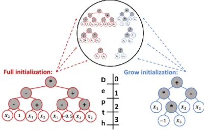
Figure 2.6: Pseudo-code for Ramped Half-and-Half initialization method. From figure2.7, the one can visually perceive how RHH works ford= 3 andP = 6. In the figure, the individuals represented in red were initialized by means of Full method, whereas those in blue by Grow method.
2.4.3.2 Evolutionary Demes Despeciation Algorithm
Initialization is known to play an important role in any population-based algorithm. In GP, this aspect plays particular importance since a wide variety of programs of various sizes and shapes is desirable [34, 42]. With the introduction of GSOs, new
2 . 4 . E V O LU T I O N A RY A L G O R I T H M
Full initialization: Grow initialization:
Figure 2.7: Example of functioning of RHH for a population of size 6 and maximum depth of 3.
techniques which take in consideration their particularities, have been developed [2,
40,54]. In this subsection we will focus on one of these contributions, the Evolutionary Demes Despeciation Algorithm (EDDA) [54], since it is the initialization technique used in our experiments.
In Biology, demes are independent populations, or sub-populations, of individuals that actively interbreed and mature. The term despeciation indicates the combina-tion of demes of previously distinct species into a new populacombina-tion, where distinct biological lineage is blended. Although in Nature the despeciation phenomenon is rare to happen, when it does, it is known toreinforcethe population making it more competitive.
In EDDA, the initial population of GSGP is generated using the best individuals obtained from a set of independent sub-populations (demes), left to evolve forfew gen-erations and under different evolutionary conditions [54]. For example, some demes use standard GP operators, while the remaining use GSOs. Besides that, each deme is being evolved under distinct search parameters such as the mutation and crossover probability, the mutation step (in the case of GSM), etc.
Although EDDA was introduced in the GP community recently, it was successfully applied when solving several fundamentally distinct problems [4–6]. GSGP using EDDA demonstrated its superiority over GP initialized with traditional Ramped Half-and-Half (RHH) [34] method over six complex symbolic regression applications [54]. More specifically, on all problems, EDDA allowed for generation of solutions with better or comparable generalization ability and of significantly smaller size than us-ing RHH. In [5, 6] EDDA demonstrated its utility when evolving PSO-based search
C H A P T E R 2 . T H E O RY
rules in unknown vector field whereas in [4] it was used to support medical decisions in the field of rare diseases.
The performance of EDDA depends on two main parameters: the proportion of GSGP demes in the system (n) and the number of generations to evolve each deme (m). Using algorithm-specific notation, given two natural numbersnandm, wheren
∈ [0,100], EDDAm−n% represents a system where demes are left to evolve for m
generations such thatn% of the population was initialized using individuals from GP demes, while the remaining (100−n)% was initialized using standard GP demes. The
pseudo-code in Figure2.8explains the process. EDDAm−n%:
1. Create an empty populationP of sizeN; 2. RepeatN∗(n/100) times:
a) Create an empty deme;
b) Randomly initialize this deme using a classical initialization algorithm (RHH used here);
c) Evolve individuals from 2.b) formgenerations using GSGP;
d) After finishing 2.c), select the best individual from the deme and store it inP; 3. RepeatN∗(1−n/100) times:
a) Create an empty deme;
b) Randomly initialize this deme using a classical initialization algorithm (RHH used here);
c) Evolve individuals from 3.b) formgenerations using standard GP;
d) After finishing 3.c), select the best individual from the deme and store it inP; 4. RetrieveP and use it as the initial population of GP
Figure 2.8: Pseudo-code ofEDDAm−n% system, in which demes are left to evolve
formgenerations.
In the pseudo-code of Figure 2.8, points 2.b), 2.c), 3.b) and 3.c) implement the phase ofdemes evolution, such that different demes are left to evolve in an independent manner. Points 2.d) and 3.d) implement the phase ofdespeciationwhere individuals, coming from different demes and thus from different evolutionaryjourneysand histo-ries, are blended into a new population (P in the pseudo-code). To evolveP, GSGP is preferred over standard GP as the later is known to outperform the former in several application domains [50, 53]. In order to confirm this evidence, in this study, after
despeciationphase, we have compared the performance of S-GP and S-GSGP systems to conduct the main evolutionary process (MEP).
The rationale behind EDDA system is that it should generate an initial population composed of diverse and, at the same time, good quality genetic material. In fact, each
2 . 4 . E V O LU T I O N A RY A L G O R I T H M
individual in the initial GSGP population comes from a different evolution history, performed in an independent deme and evolved under different search parameters. Given that each individual in the initial GSGP population was the best individual in its deme, good quality is expected.
2.4.4 Parent Selection
The parent selection is the mechanism allowing only the individuals with the best features for a given problem to become parents and to produce offspring with certain inherited traits. In this experimentation, the Tournament and-Lexicase methods were used.
2.4.4.1 Tournament
In Genetic Programming, Tournament is the most popular selection method. First, a defined number (Tournament size) of individuals in the population is randomly selected. Then, only the individuals with the best fitness in this intermediary group are picked to become parents. The genetic operator crossover for instance, uses 2 parents, so 2 tournaments need to be done. The selection pressure is the ratio between the number of individuals in the population and the number of individuals randomly selected by the tournament method. It measures the chance of any individual to participate in the tournament.
2.4.4.2 -Lexicase Selection for Regression
-Lexicase Selection (-LS) [36] is a recently introduced improvement upon already existing Lexicase Selection (LS) of parents in GP [47]. The latter was proposed by Lee Spector in 2012 to provide a simple, problem and representation-independent way to solve multimodal problems without interfering with other components of a GP system. In simple terms, LS is an iterative procedure which consist of the following steps:
Letdi be thei-th data instance (a.k.a. fitness case) taken in random order from training dataset DtrainandSi the selection pool at iterationi, initially composed by the whole population:
1. f or di in Dtrain:
a) evaluate all candidate solutions inSi ondi;
b) remove those candidate solutions fromSi whose fitness is worse than of the
best-found solution;
2. ifScontains more than one candidate solution, return one at random.
Figure 2.9: Pseudo-code for Lexicase Selection (LS) technique.
The underlying assumption embedded in LS is that problem’s multi-modality is, at least partially, a factor of its fitness cases, each of which represents a circumstance with which acorrectsolution must deal. As such, different subsets of fitness cases may
C H A P T E R 2 . T H E O RY
call for differentmodes of response, i.e., may require the system to respond in a different manner. Under the light of this assumption, extension of lexicographic ordering to the fitness cases in randomized order ensures that agoodfitness, calculated on a given case
di, will be rewarded independently on solution’s performance on other cases, while, at the same time, still rewarding the progress on a larger set of fitness cases (up to the size of training dataset).
By looking at the pseudo-code in 2.9, one can identify technique’s vulnerability when dealing with regression problems: in regression, exact solutions to fitness cases can mostly be expected fortoyproblems, whereas real-world problems are often sub-ject to noise and measurement error. As such, when applied on real-world regression problems, the standard LS typically uses only one fitness case for each parent selection, resulting in poor performance [36]. To deal with this limitation, authors in [36] pro-posed torelaxthe passing criteria (fromSitoSi+1) by introducing a parameter, such
that only individuals inside a predefinedare selected forSi+1. In their work, authors
proposed four different definitions of and assessed their performance, along with four state-of-the-art techniques, on 3 synthetic and 3 real-world regression problems. The experimental results allowed to identify the most performing definitions ofand proved the effectiveness of proposed technique when compared to state-of-the-art.
Given the results presented in [36], we decided to choose -LS with Automatic Threshold Adaptation (ATA) defined as semi-dynamic. Although authors did not find a statistically significant difference with another version of ATA, defined as dynamic, we decided to opt the former as semi-dynamic, as it has been defined as default solution by the author.
semi-dynamic formula:= median(abs(error_pop - median(error_pop)))
2.4.5 Fitness Evaluation
The Fitness function is used to evaluate how close a prediction is to the actual value. The main goal is to drive the algorithm to the optimal solution. In GP and GSGP, when used for regression, the prediction is a vector of continuous values. The fitness function compares the individuals of the population in order to find the elite (individual with the best fitness in the population). During the evolution process, it helps to design the solution of the algorithm. Since it’s used for each individual and at every step of the evolutionary process, it has to be fast to save some computation time.
2.4.6 Elitism
The strategy of elitism is to maintain the best element observed so far through all generations. After the parent selection and the genetic operator variations, a new
2 . 4 . E V O LU T I O N A RY A L G O R I T H M
population of offspring is created. The fitness evaluation of each offspring allows for the best individual of the new population to be determined. Best individuals from the current and previous generation are compared with their fitness for the training data. The elite of the previous generation will replace randomly an individual of the new population only if its fitness is better than the best individual of this population. This way the best solution observed still has a chance to produce offspring in the next generation.
2.4.7 Semantic Stopping Criterion
If the model’s behavior on unseen datahighly differs from the one on training data, one can say itlacks generalisation. This can be caused by many factors, among them, in the context of EAs, an inappropriate number of iterations. In fact, after a given point, furthermachine learningon available data can potentially make the modeloverfit, i.e. memorize the training data instead of generalizing from it.
Semantic Stopping Criterion (SSC) is a recently proposed stopping criterion [23] which operates in the context of GSOs, described in2.4.2and further extended in the context of neuroevolution [24]. More specifically, to decide when to stop, SSC uses in-formation gathered from thesemantic neighborhood, a set ofsemantic neighboursof the current-best solution in terms of training data, which are obtained by means of GSM. Authors propose two types of SSC: Error Deviation Variation (EDV) and Training Im-provement Effectiveness (TIE). The first measures the percentage of those neighbors that, besides beingfitterthan the current-best, have a lower sample standard deviation of the absolute errors. The second measures the percentage of times the underlying semantic variation operator, in our case GSM, is able to produce a neighbor that is su-perior to the current-best. In both versions, only training data is considered for fitness calculation. The experimental results proved that the proposed stopping criteria are able to achieve acompetitivegeneralization on the set of problems considered in their experiments, however no clear conclusions were provided regarding which of the two criteria is preferred. For this reason, and because computational effort for computing EDV nearly implies computation of TIE, we decided to assess both variants.
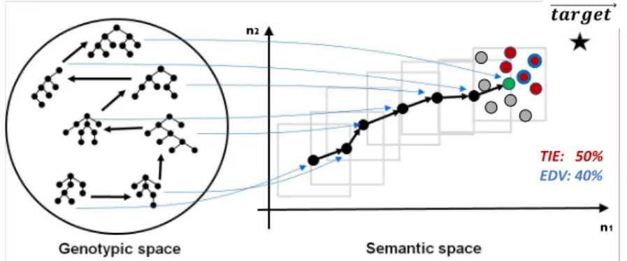
Figure2.10illustrates functioning of both SSC’s variants - EDV in blue and TIE in red. Consider current-best solution at iterationi represented as a green point in 2D semantic space. Assuming a neighbourhood size of 10, the points generated within the gray box represent its semantic neighbors. Those represented in red, regard to semantic neighbors which are better than the current-best; since they are 5 out of 10, TIE is 50%. Those represented in red with a blue contour, regard to those neighbors that, besides being better than the current-best, have a lower sample standard deviation of the absolute errors; since they are 2 out of 5, EDV is 40%. Assuming the latter was
C H A P T E R 2 . T H E O RY
chosen as the stopping criterion with a threshold value of 50%, the search would stop at iterationi.
TIE: 50% EDV: 40%
n1
n2 𝒕𝒂𝒓𝒈𝒆𝒕
Figure 2.10: Illustration of SSC’s functioning. Thestar in the figure represents the target vector on training data.
2.4.8 Genetic Programming as a Meta-Learning Technique
It is known that maximal generalization ability of an ensemble can be achieved through
prudentcombination ofdiverseBLs. Many ensemble methods, however, require their manual selection, parametrization and combination. This means that full potential of this combination ofsearch-paradigmsin generatingsynergisticeffects might be under-explored. In this light, GP can be seen as aneffective assembling method due to its
flexiblerepresentation,highinterpretability of evolved solutions andpowerful induc-tive capabilities. To explore GP’s role as a meta-learning technique, one has fulfill a fundamental requisite: to build the set of terminals from the combined predictions of several distinct base-learners.
The use of GP as an automatic EL technique is not new in the research field. To our knowledge, the first evidence comes from 2006 [26], when GP was used to combine 10 ANNs into an ensemble. Through experiments’ analysis, anotorious superiority of the proposed approach was verified, when evaluated on 22 publicly available real-world SML problems. In [12], authors compared an equivalent approach against 3 ensemble approaches based on GAs. The experimental results involving 4 synthetic and 1 real-world symbolic regression tasks confirmed the preeminence of GP-based ensemble not only against the best BL, which was an ANN, but also the three different types of GA-based ensembles.
In [20], authors extended the usage of GP to learn ensemble policies by using up to 6 heterogeneous BLs, some of which ensembles themselves (which was the case of
2 . 4 . E V O LU T I O N A RY A L G O R I T H M
Random Forest), and assessed system’s performance on 10 synthetic symbolic regres-sion problems. Additionally, in attempt to increase the synergistic effect of combining different BLs into an ensemble policy, authors proposed a novel operator entitled as
decision expression, which splits the input space into sub-spaces that can then be han-dled by different sub-policies. Despite of their expectations, their approach performed significantly better than the best BL only at one problem. While on the remaining problems the performance of their system was comparable or worse. In their work, authors pointed several limitations, namely the overfitting - perceived by the fact GP simply selects from the BLs instead oflearningacomplexandmeaningfulpolicy - and the absence of real-world benchmark problems. The latter translates in the absence of potentiallychallengingfitness landscapes for the BLs, a scenario which seems suitable for the method they have proposed. Despite of carrying, in our opinion, an important contribution, for our surprise, this work was not published neither in a conference or a journal...
In [44] authors exploited the fact that semantics, defined in 2.4.2 as the vector of output values of a candidate solution calculated on the training observations, are independent from the underlying model and proposed an extension to GSGP, called Universal-GP (U-GP) in which some initial individuals are created by means of exter-nal programs, i.e., other ML techniques. More specifically, authors proved that, by producing semantics using fundamentally distinct ML models, in this context seen as BLs, and including them in the initial population of GSGP’s evolutionary process along with random initial programs, it is possible to obtain a significant improve-ment over standard RHH initialization. It is also important to point that, after iden-tifying system’s sensibility towards overfitting of BLs, authors have introduced the
pre-evolutionary selection procedure, referred as PESP, which attempts to exclude from the evolution those BLs which are unable to individually achievegoodgeneralization performance after training and after a short run of GSGP. This approach, which essen-tially introduces an additional level of cross-validation, allowed the system to achieve superior performance when compared to standard S-GP on 4 real-world regression problems.
All aforementioned contributions, except [44], can be categorized as stacking, where standard GP assumes the role of a meta-learner from the combined predic-tions of several BLs. For this reason and from this moment on, we will entitle these kind of approaches as Stacking-SGP (S-SGP). Taking in consideration the information presented in the next section and to facilitate the reading of this document, we will use the nomenclature Stacking-GSGP (S-GSGP) for those cases when GSGP assumes the role of a meta-learner and Stacking-GP (S-GP) for any GP-based approach to combine the predictions of several BLs.
C
h
a
p
t
e
r
3
M e t h o d o l o g y
3.1
Proposed approach
As it was mentioned in 2.2.1, in this paper we explore S-GP; nevertheless, this paper presents several fundamental differences regarding the previous work. Since the first usage of S-GP [26], the research field in GP has dynamically evolved and several new approaches have emerged. Geometric-Semantic Operators (GSO), Semantic Stopping Criterion (SSC),-Lexicase Selection (-LS) and Evolutionary Demes Despeciation Al-gorithm (EDDA), the methods appear enumerated in ascending order of their recency, are among numerous examples of recent achievements of the scientific community in the research field. The first fundamental difference, hence a scientific contribution, consists of applying and comparing these novel achievements, assessing their eff ec-tiveness on the underlying tasks, as such updating the state-of-the-art in the research field. The second if related to the fact that none of the previous work provides a con-cise benchmark over regression problems when using S-GP: in [1,29] authors study the effectiveness of their approach under the light of classification problems, whereas in [20] authors only cover synthetic regression problems. Apart from updating field’s state-of-the-art, we also provide a concise overview of 7 synthetic and 4 real-world regression problems, which complements the scientific panorama in the research field.
3.2
Objectives
The experimental environment is built upon 7 synthetic and 4 real-world regression problems and the experiments were conducted to accomplish the following six objec-tives:
C H A P T E R 3 . M E T H O D O L O G Y
1. Identify and characterize hyper-parameter sets of S-GSGP which exhibit the high-est performance on all the problems simultaneously, and on real-world and syn-thetic problems separately;
2. Compare the performance between different GP-based techniques in the con-text of stacking, namely: RHH initialization, Tournament selection (TS) and traditional Stopping Criteria with recently introduced EDDA,-LS and SSC, re-spectively;
3. Assess the validity of GSOs, in the context of stacking by comparing them with standard GP operators;
4. Compare system’s performance against BLs, some of which ensembles them-selves (which is the case of Random Forest);
It is important to highlight that, in order to assess systems’ generalization ability, the experiments were conducted involving both training and unseen data instances.
3.3
Ensemble hyper-parameters
Table 3.1 provides an exhaustive enumeration of hyper-parameters that were used in our experiment for all the problems (both synthetically-generated and real-world). It is important to notice that during experimental phase we have performed an ex-haustive search over the following parameter values: Meta-Learner, BLs pre-training,
Initialization,Selection,P(Crossover) andStopping criteria, while maintaining all other parameters fixed. This means that a single execution of the benchmark environment, i.e., one run, implies 128 experiments for each of 11 considered problems (which yields a total of 1408 experiments per run). Throughout our experiments we guaran-teed an equal number of fitness evaluations for all the types of S-GP systems studied - 70000 generations. For a S-GP system which uses RHH initialization technique this computational resource results in 500 generations for a population size of 140 (i.e., 500x140 = 70000). Similarly, for a S-GP system where initialization is performed by means of EDDA technique with maturation of 5 generations and percentage of GSGP demes equal to 50% (EDDA5−50%), this computational resource results in 200
gener-ations for a population size of 100 (i.e., 100x5x100 + 200x100). The stopping criteria was compared after executing the experiments for the number of generations specified in the table (see№generations).
Having in mind the stochastic nature of employed algorithms and results’ volatility upon data partition, i.e., to provide a robust and statistically-consistent analysis of ex-perimental results, we repeated the experiments 60 times (runs), each with a different
3 . 4 . E X P E R I M E N TA L P R O B L E M S
pseudo-random number generator (a.k.a. seed), used for partitioning the data, and algorithms’ initialization and execution.
Parameters Values
№runs 60
Meta-Learner S-SGP, S-GSGP
№generations 500RHH, 200EDDA5−50%
Population size 140RHH, 100EDDA5−50%
Function set add, sub, mul, avg, min, decision BLs set LR, SVM, RF, MLP
Tuned BLs True, False
Initialization RHH,EDDA5−50% Selection TS,-LS Crossover Swap, GSC Mutation Subtree, GSM P(C) 0, 0.2, 0.8, 1.0 P(M) 1−P(C)
Stopping criteria TIE, EDV, validation fitness,№generations
Table 3.1: Enumeration of hyper-parameters. It is worth to notice thatdecisionstands for the decision expression operator proposed in [20], BLs pre-training indicates if the BLs were tuned or not,-LSrepresents the selection algorithm proposed in [36],
P(C) andP(M) indicate the crossover and mutation probabilities, andvalidation fitness
stands for the stopping criteria which operates upon the fitness calculated from vali-dation partition by estimating the point from where further induction allows further generalization.
3.4
Experimental Problems
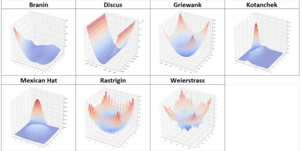
In this section, the reader can find a detailed characterization of the experimental problems we used in our experiments. Table3.2contains the mathematical formula-tion for 7 synthetic regression problems used in this study, whereas tables3.3and3.1
complement the latter by specifying their bounds (the domain) and providing a graph-ical visualisation of the fitness landscapes. It is worth to highlight that these functions were studied in two dimensional input space. For each of these problems, we have generated 200 two-dimensional data points under Continuous Uniform Distribution where parameters for each dimension were chosen from table3.3. Then, these points were used as the input for the functions defined in table3.2to generate the respective target vectors. As a result, each synthetic regression problem is defined by 200 data ob-servations characterized in two-dimensional input feature-space and one dimensional output.
Table 3.4 summarizes the 4 real-world regression problems. The Boston prob-lem [48] is from the field of real estate analysis and it consists of predicting the value of owner-occupied homes in suburbs of Boston, a city in United States of America, as
C H A P T E R 3 . M E T H O D O L O G Y Name f(x1, x2) Branin ax2−bx2 1+cx1−r 2 +s(1−t)cos(x1) +s Discus x21106+x22
Griewank 1 +40001 x12+40001 x22−cos(x1) cos(1
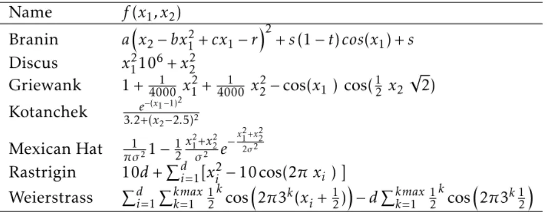
2 x2 √ 2) Kotanchek 3.2+(e−(xx1−1)2 2−2.5)2 Mexican Hat πσ121−12 x2 1+x22 σ2 e −x 2 1 +x22 2σ2 Rastrigin 10d+Pd i=1[x2i −10 cos(2π xi) ] Weierstrass Pd i=1 Pkmax k=1 12 k cos2π3k(xi+12)−dPkmax k=1 12 k cos2π3k12
Table 3.2: Mathematical formulation of synthetic regression problems used in this study. The problems are listed in alphabetical order.
Bound: Lower Upper
Problem x1 x2 x1 x2 Branin -5 0 10 15 Discus -32.786 -32.786 32.786 32.786 Griewangk -600 -600 600 600 Kotanchek -2 -1 7 3 Mexican Hat -5 -5 5 5 Rastrigin -5 -5 5 5 Weierstrass -0.5 -0.5 0.5 0.5
Table 3.3: Enumeration of search space’s boundaries (the domain) for each function. It is worth to notice that columnsLowerandUpperstand for lower and upper bounds of two dimensional search space.
a function of its geographic, socioeconomic, environmental and housing characteris-tics. TheDiabetesproblem [37] contains blood pressure and demographic data of 442 persons who happen to have diabetes and the target value is a quantitative measure of disease progression one year after the baseline measurement. ThePPBproblem [22] comes from the field of pharmacokinetics and consists of predicting the percentage of the initial drug dose which binds plasma proteins as a function of its 626 molecular descriptors. Finally, the Parkinson problem [49] is mostly composed of biomedical voice measurements from 42 people who, at the time of data-collection, happened to have Parkinson’s disease at its early stage. They were recruited to a six-month trial of a tele-monitoring biomedical speech recording device for remote symptom progression monitoring. The objective is to predict Parkinson’s symptom progression measured through total Unified Parkinson’s Disease Rating Scale (UPDRS).
We considered to include these problems in our study as all of them have been target of research using several different ML techniques, they are significantly diverse and, in the case of real-world problems, are considered ofhigh importance in their respective industries.
3 . 5 . P R O B L E M DATA S E T - T R A I N A N D T E S T S P L I T
Figure 3.1: Optimization Problems Dataset (ID) #Features #Instances Field
Boston 13 506 Real Estate
Diabetes 10 442 Medicine
PPB 626 131 Pharmacokinetics
Parkinson 20 5876 Medicine
Table 3.4: Description of real-world regression problems used in the experiments. For each problem, the name (ID), number of input features (#Features), data instances (#Instances) and field of application (Field) is presented.
3.5
Problem dataset - Train and Test split
In the workflow of the experiment (figure A.1), we can see that each dataset has to be split into two parts3.2, the training set used to train the base learners during the learning process, and the testing set which remains during the training but used for the final prediction.
Listing 3.1: Python code for Train and Test split
1 from sklearn . model_selection import train_test_split
2 X_train , X_test , y_train , y_test
3 = train_test_split (X , y , test_size =0.3 , random_state = run_number )
The function ‘train_test_split’ from Scitkit-Learn shuffle randomly and split the given arrays ‘X’ and ‘y’ using the common rule of thumb 70/30. Meaning that 70% of data will be used for the training set, output arrays ‘X_train’ and ‘y_train’, and 30% the testing set, output arrays ‘X_test’ and ‘y_test’. The random state ensures that at each run the random distribution will be different.
C H A P T E R 3 . M E T H O D O L O G Y
Dataset - 200 points
Training 70% - 140 points Testing 30% - 60 points
Figure 3.2: Dataset split representation
This way the dataset of 200 points is split into two parts, the training set of 140 points and the testing set of 60 points.
3.6
Base Learners hyper-parameters tuning
Hyper-parameter tuning is the fact of finding the right settings of a model for a specific dataset.
In a separated process from the workflow, only the problem training dataset is used.
GridSearchCV a module from Scikit-Learn (same library as the base learners) al-lows trying different parameters for a given model and dataset. A cross-validated score is given to all combinations of parameters, confirming that the best parameters set will perform well on different samples of the dataset. For each problem, the best parameter set is saved and used if the variable Tuned is set at True.
When not Tuned the base learners use their default hyper-parameters values which are not optimized for the given dataset, resulting in potentially bad performance.
3.7
Base Learners dataset - K-Fold data generation
As shown in the workflow of the experiment (figureA.1), after the problem dataset split, the base learners are trained with only a part of the training dataset because we want to output predictions based on unseen data also coming from the same training set. If the data to be predicted has already been seen during the training, the outputted predictions will be unrealistic and the ensemble will overfit for unseen data.
Using a K-fold technique, the training set is divided into K parts. For the base learners, K minus 1 folds are used as inputs during the training, and 1 fold is used as input for the prediction. We chose to use 10 folds, so the base learners are trained 10 times, to predict the target of 10 different folds.