Cloud base height estimates from sky imagery and a network of pyranometers

UC San Diego

UC San Diego Previously Published Works

Title

Cloud base height estimates from sky imagery and a network of pyranometers

Permalink

Journal

ISSN

Authors

Publication Date

DOI

Cloud base height estimates from sky imagery and a network of

pyranometers

Guang Wang, Bryan Urquhart, Jan Kleissl 5

Center for Renewable Resources and Integration, Department of Mechanical and Aerospace 6

Engineering, University of California, San Diego, United States 7

8 9

Abstract

10

Cloud base height (CBH) is an important parameter for physics-based high resolution solar 11

radiation modeling. In sky imager-based forecasts, a ceilometer or stereographic setup is needed 12

to derive the CBH; otherwise erroneous CBHs lead to incorrect physical cloud velocity and 13

incorrect projection of cloud shadows, causing solar power forecast errors due to incorrect 14

shadow positions and timing of shadowing events. In this paper, two methods to estimate cloud 15

base height from a single sky imager and distributed ground solar irradiance measurements are 16

proposed. The first method (Time Series Correlation, denoted as “TSC”) is based upon the 17

correlation between ground-observed global horizontal irradiance (GHI) time series and a 18

modeled GHI time series generated from a sequence of sky images geo-rectified to a candidate 19

set of CBH. The estimated CBH is taken as the candidate that produces the highest correlation 20

coefficient. The second method (Geometric Cloud Shadow Edge, denoted as “GCSE”) integrates 21

a numerical ramp detection method for ground-observed GHI time series with solar and cloud 22

geometry applied to cloud edges in a sky image. CBH are benchmarked against a collocated 23

ceilometer and stereographically estimated CBH from two sky imagers for 15 minute median-24

filtered CBHs. Over 30 days covering all seasons, the TSC method performs similarly to the GCSE 25

method with nRMSD of 18.9% versus 20.8%. A key limitation of both proposed methods is the 26

requirement of sufficient variation in GHI to enable reliable correlation and ramp detection. The 27

advantage of the two proposed methods is that they can be applied when measurements from 28

only a single sky imager and pyranometers are available. 29

30

Keywords: Cloud base height; Sky imager; Irradiance ramp detection; Short-term solar forecasting 31

33

Nomenclature

34

GHI$(𝑡; 𝐻) GHI simulated using USI imagery at a _{given CBH} 𝑡* Current time

GHI$+,-(𝑡) GHI from the pyranometer at station 𝑖 𝐮0 Cloud pixel speed [pixel s-1] GHI$1-2(𝑡) GHI from clear sky model 𝐮 Cloud speed [m s-1]

𝐻 Cloud base height (CBH) 𝐱4 Intersection of cloud motion line and cloud _{boundary [m]}

𝐻1567 _{CBH measured by ceilometer 𝐱8}

4 Intersection of cloud motion line and cloud _{boundary [pixels]} 𝐻9 CBH candidate 𝐱: Vector describing ground station location _[m] 𝐻;+<57

CBH estimate from Time Series Correlation and Geometric Cloud Shadow Edge methods

𝐱8: Vector describing ground station location _[pixels] ℎ Sky imager elevation 𝐱> Intersection of solar beam and cloud map 𝐾 Number of samples in 20 minutes at 30 _{second intervals} Δ𝐻 Cloud base height error [m]

kt Clear sky index ∆𝑡

Cloud travel time, a time difference between given initial timestamp 𝑡$ and start of next down ramp

M Number of modeled CBH values ∆𝑡F Forecast time step

MBE Mean bias error ∆𝐱

Cloud shadow horizontal shift

corresponding to cloud base height vertical shift Δ𝐻 [m]

𝑛_J Number of cloud map pixels in one

dimension ∆𝐱8

Cloud displacement in the sky image [pixels]

N Total number of available ground sites Δ𝐱4 Cloud projection error

nMBE Normalized mean bias error 𝜃 Zenith coordinates of a pixel in the sky image

nRMSD Normalized root mean square _difference 𝜃Q Sky imager field of view in degrees from the _vertical

𝑂 Sky imager position 𝜃> Solar zenith angle

𝑅 Length of cloud map in one dimension 𝜆 Distance along a ray from observation point 𝑅$9

Correlation coefficient between GHI6U𝑡; 𝐻9V and GHI$+,-(𝑡)at site 𝑖 for CBH 𝐻9

𝜇 Cloud velocity scaling factor 𝑅9

Correlation coefficient averaged over all

sites at CBH 𝐻9 𝜇$

+,- _{Mean of GHI} $ +,-_(𝑡) RMSD Root mean square difference 𝜇$9 Mean of GHI$U𝑡; 𝐻9V

𝑡 Time 𝜙 Azimuth coordinates of a pixel in the sky _image

𝑡$ Initial timestamp used to compute ∆𝑡 𝜙> Solar azimuth angle 35

1.

Introduction

36

1.1

Impact of CBH on Intra-hour Solar Power Forecasting with a Sky Imager

CBH plays a vital role in intra-hour solar power forecasting. For typical mid-latitude solar zenith 38

angles of 45°, a difference of 100 m in CBH causes a 100 m translation of the cloud shadow on 39

the ground (Eq. (1). In addition, since opaque clouds typically have a clear sky index of 0.4, local 40

power output forecast errors of 60% of clear sky production levels (Martinez-Anido et al., 2016) 41

are common if a CBH error causes the wrong sky condition (clear or cloudy) to be forecast. Thus, 42

accurate CBH estimation is critical for predicting local power ramps over short time scales. 43

For sky imager solar forecasts that are based on the geometry between the sun, clouds, and 44

ground, CBH is required for mapping the cloud field from sky images to the atmosphere and then 45

projecting to the ground. Specifically, the mapping process consists of three geometry steps: 1) 46

projection of the clouds in the sky image into a plane in the sky (termed “cloud map”, see Section 47

2.3) at the CBH; 2) forward motion of the cloud map in time; 3) projection of cloud map onto the 48

ground. Thus, an erroneous CBH leads to three different scaling errors listed below (see the 49

nomenclature for variable definitions and Section 3.2. for derivations: 50

51

1) The cloud projection error is: 52

Δ𝐱1= 𝛥𝐻 ∙ (𝑡𝑎𝑛 𝜃 𝑠𝑖𝑛 𝜙 , 𝑡𝑎𝑛 𝜃 𝑐𝑜𝑠 𝜙 , 1)b (1)

where Δ𝐱1 is a 3D-vector describing position error for a given CBH error ΔH, and (𝜃, 𝜙)

53

are respectively the zenith and azimuth pointing angles corresponding to a pixel obtained 54

using pixel coordinates (refer to Figure 4 later) and the camera geometric calibration (e.g. 55

Urquhart et al. 2016). ΔH linearly scales cloud horizontal position in the radial direction 56

and stretches or shrinks the cloud about a center point at the sky imager, and the scaling 57

error is more sensitive to ΔH at farther spatial distance (outer pixels) caused by the 58

nonlinear effect of 𝑡𝑎𝑛 𝜃. 59

60

2) Physical cloud velocity error. Because the cloud velocity derived from sky image is in units 61

of pixels, a conversion to actual cloud velocity in units of m/s requires scaling the pixel 62

velocity with CBH, resulting in a linear scaling error by 𝛥𝐻. 63

64

3) Cloud shadow projection error. When the cloud map is advected and projected onto the 65

ground, the vertical shift ∆𝐻 causes a uniform horizontal shift |∆𝐱| in shadow position 66

|∆𝐱| = ∆𝐻 𝑡𝑎𝑛 𝜃_>, (2) which is exaggerated at larger solar zenith angles 𝜃_>. Thus, CBH errors also cause 68

shadows or sunlight to be predicted at locations that are shifted further as the distance 69

from the sky imager increases. 70

71

1.2

CBH Measurement Techniques

CBH can be measured directly using in-situ and remote sensing instruments such as 73

radiosondes (Wang & Rossow, 1995), ceilometers (Gaumet et al., 1998; Martucci et al., 2010), 74

and satellites (Hutchison et al., 2006). A radiosonde is a battery-powered telemetry instrument 75

package that vertically profiles the atmosphere as the balloon ascends, yielding CBH estimates. 76

Although the CBH measurements from a radiosonde are accurate, the observations are usually 77

taken at most twice daily and at discrete and sparse locations, making them unsuitable for use in 78

intra-hour solar energy forecasting. Ceilometers are the most common CBH observational tool 79

and are regularly installed at airports and meteorological aerodrome reports (METAR) stations. It 80

emits a pulsed near-infrared vertical laser beam and measures a vertical profile of atmospheric 81

backscatter from which CBH is derived. Since ceilometers can be expensive, they have limited 82

application outside of airports in most countries except in the UK, where ceilometer is a standard 83

component of weather stations. 84

Indirect CBH measurements using ground based thermal infrared cameras (Shaw and Nugent, 85

2013; Liu et al., 2015) and derived data from remote-sensing techniques such as 86

spectroradiometers (Hutchison et al., 2006) are also feasible. The assumption that clouds are 87

blackbodies usually leads to an overestimation of CBH derived by infrared cloud imagers (Liu et 88

al., 2015). Satellite-measured cloud top near-infrared radiance (Dessler et al., 2006) or measured 89

cloud top temperature with an atmospheric temperature profile (Prata & Turner, 1997) can be 90

used to obtain cloud top height with wide spatial coverage, but CBH is difficult to detect from 91

satellites and time delays in data dissemination limit its application in short-term solar power 92

forecasting. Numerical weather prediction offers another alternative to obtain CBH (Killius et al., 93

2015). 94

CBH can also be obtained from sky imagery. The application of stereogrammetric techniques 95

using two sky imagers was investigated by Allmen and Kegelmeyer (1996) and Kassianov et al. 96

(2005). Nguyen and Kleissl (2014, referred to as NK14) further generalized and improved 97

accuracy and computational efficiency of the approach introduced by Kassianov et al. (2005) for 98

(binocular) stereographic CBH estimation: a two-dimensional (2D) georeferenced projection is 99

used to overlay images from each camera. The CBH is the cloud height associated with the 100

minimum normalized matching error, which implicitly assumes a single cloud layer. More 101

sophisticated stereo-vision techniques can offer cloud base height estimate in 3D coordinates 102

using the standard technique of matching image patches along epipolar curves (Allmen and 103

Kegelmyer, 1996; NK14; Kleissl et al., 2016). These methods are computationally intensive and 104

provide high spatial resolution CBH within a pair of images. The stereographic method requires 105

at least two sky imagers and accurate geometric calibration of the imaging system (e.g. Urquhart 106

et al., 2016). Wang et al. (2016) and Kuhn et al. (2018a; 2018b) demonstrated that CBH can be 107

obtained from a single sky imager and an independent measurement of cloud speed. Because 108

angular cloud speed determined from sky images is proportional to cloud speed and CBH, CBH 109

can be derived from a collocated cloud speed sensor (Fung et al., 2014) and sky imager. In Wang 110

et al. (2016) and for the same location as in this paper, typical daily root mean square differences 111

were 126 m or 17% of the observed CBH. But the raw (instantaneous) CBH measurements need 112

to be filtered to derive a robust CBH, which makes CBH outputs infrequent (one CBH output every 113

50 sec for 27 partly cloudy days and every 250 sec for 21 overcast days, on average). 114

1.3

Objectives and Structure of the Paper

CBH is a required input for some sky imager-based short-term solar power forecasting 116

variants (Chow et al., 2011; Schmidt et al., 2016). The variety of methods presented in Section 117

1.2 can produce accurate CBH information at different temporal and spatial scales, however either 118

equipment or operating costs are prohibitive, or computational requirements are high, or the 119

temporal resolution is insufficient for intra-hour solar power forecasting. 120

Cameras are ubiquitous and low cost, and nearly every solar power installation has 121

pyranometers and PV energy meters. Therefore, existing and low cost infrastructure provides an 122

opportunity to estimate cloud height as an ancillary product if the irradiance distribution on the 123

ground is measured in space and time. Thus, the objective of this work is to provide a low-cost 124

alternative to estimate CBH using such irradiance measurements and a single sky-pointing 125

camera. CBH is estimated using two related methods requiring a single sky imager and irradiance 126

sensors distributed within the footprint of the sky imager, i.e. within the camera’s field of view. 127

Both methods are new and have not been been presented before. In the first method, CBH is 128

estimated by correlating ground-observed GHI measured using a set of pyranometers with GHI 129

modeled using a sky imager irradiance forecast (Chow et al., 2011). Modeled GHI time series are 130

generated from a sequence of sky images geo-rectified to a candidate set of CBH. The second 131

method estimates CBH by matching ramp event timings from pyranometer-measured GHI to 132

cloud shadow arrival times derived from cloud geometry and sun triangularization adapted to sky 133

imagery. The presentation of the latter method provides a new mathematical description of the 134

forecast approach used in Chow et al. (2011). 135

This paper is organized as follows. The measurement equipment, including the sky imaging 136

system and forecasting procedure, is briefly described in Section 2. Section 3 introduces the CBH 137

estimation methods. Section 4 presents the overall performance in a set of 30 days, and then 138

validates CBH from both methods against ceilometer data and the NK14 stereographic method 139

in a case study. Section 5 provides detailed discussion regarding the performance and limitation 140

of the proposed methods. Finally Section 6 provides conclusions and future work. 141

2.

Experimental Data and Sky Imager Forecast Procedure

142

2.1

Ground Measurements

The University of California, San Diego (UCSD) designed and developed a sky imager system 144

specifically for short-term solar power forecasting applications (Fig. 1, Urquhart et al., 2013). The 145

UCSD Sky Imager (USI) features a high-quality image sensor and lens contained in a thermally 146

controlled, compact environmental housing, and capture software employing a high dynamic 147

range (HDR) imaging technique. The USI uses an Allied Vision GE-2040C camera which has a 148

15.15 × 15.15 mm ON Semiconductor KAI-04022 CCD sensor (originally developed by Kodak). 149

The Sigma 4.5 mm focal length fisheye lens provides a 180 degree field of view with 1748 × 1748 150

pixels covering the sky hemisphere. Thermal stability of the camera is achieved using two 151

thermoelectric coolers for the entire enclosure, a copper heat sink, and a fan attached to the 152

camera to keep it at the ambient enclosure temperature. The dome on the USI is a 1.6 mm thick, 153

neutral density (ND2) acrylic hemisphere with a UV protective coating. Additional information can 154

be found in Urquhart et al. (2015). The USI used in this analysis is installed next to one of the six 155

pyranometers shown in Figure 2 and Table 1. 156

(a) (b)

Figure 1: The University of California, San Diego Sky Imager (USI). (a) Outer view showing the enclosure with dome and white radiation shields for the coolers; (b) a top view of the open system showing the components inside the enclosure.

158

GHI data sampled at 1 Hz is obtained from six weather stations with Li-COR 200SZ 159

pyranometers installed at the locations shown in Figure 2 and Table 1. In addition, a Vaisala 160

CT25K ceilometer located on EBU2 computes CBH every 20 seconds from backscatter returns. 161

Due to the small sampling area (a small <0.1° cone above the ceilometer), the heterogeneity of 162

cloud field, as well as cloud formation and movement, the 20-second ceilometer output is not 163

always representative of the CBH in the field of view of the sky imager. Therefore, consistent with 164

NK14, a 15-minute median filter is applied to ceilometer measurements prior to comparison with 165

the proposed methods. 166

167 168

Figure 2: Locations of the six pyranometers and the USI on the UCSD campus. The ceilometer is located on EBU2. Reprinted with permission from Yang et al. 2014. © Google Maps.

169

Table 1: Locations of USI and pyranometers used for CBH estimation and their respective distances to the USI. (re-tabulated with permission from Yang et al. 2014)

Station Name Latitude Longitude Altitude (m MSL) Distance to USI (m)

USI 32.8722 -117.2410 140 - BMSB 32.8758 -117.2362 111 603 CMRR 32.8806 -117.2353 111 1074 EBU2 32.8813 -117.2330 101 1257 HUBB 32.8672 -117.2534 24 1288 MOCC 32.8784 -117.2225 103 1857 POSL 32.8807 -117.2350 110 1103 170

2.2

Evaluation Dataset

The CBH estimation methods are evaluated using two different sets of CBH measurements: 172

(1) an on-site ceilometer on 33 days and (2) the NK14 2D stereography method on 3 days. Thirty-173

three cloudy days from 2012 to 2016 were selected based on the following criteria: 174

1) Data availability from sky imager, ceilometer and pyranometers. 175

2) Cloudy conditions: clear and rainy days were excluded. 176

3) Cloud type: opaque clouds such as stratocumulus, cumulus, and stratus, since they are 177

most relevant to solar forecasting of GHI that is the subject of this paper. 178

4) Cloud height predominantly less than 1000 m. Four days were chosen with cloud heights 179

greater than 1000 m 180

5) Lack of rain: less than 2 hours of rain 181

Finally, only time periods with solar zenith angles less than 75° are considered. Moreover, 182

during an intensive operating period in 2012, two sky imagers were installed, which allowed 2D 183

stereography to be applied to four days, as reported in NK14. December 14, 2012 was 184

characterized by broken stratocumulus clouds above a few cumulus clouds. On December 26, a 185

single layer of low scattered cumulus clouds was observed. December 29 was overcast with 186

stratus clouds. Jan 1, 2013 analyzed in NK14, was not included in this paper because several 187

station outages limited GHI measurements to only two stations. 188

2.3

Sky Imager Forecast Procedure

The USI can be used to geolocate clouds, to measure cloud angular velocity, and to track 190

cloud motion (Chow et al., 2011; Chow et al., 2015). These measurements are then used to 191

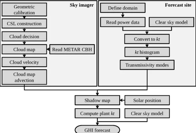
forecast future cloud locations up to 15 minutes ahead. The forecast procedure is outlined in the 192

flow chart of Figure 3. A brief overview of the USI forecast procedure is given in the remainder of 193

this section. For more information, the reader is referred to Chow et al. (2011), Ghonima et al. 194

(2012), Urquhart et al. (2013), and Yang et al. (2014). Similar sky imager systems and forecast 195

procedures can be found in Cazorla et al. (2010); Marquez and Coimbra (2013), and Schmidt et 196

al. (2016). 197

Figure 3: Flowchart of USI forecast procedure. Sky image processing (left) is combined with the clear sky index (kt) from local ground observations (right) to produce spatial irradiance forecasts. (reprinted with permission from Yang et al. (2014))

199

Based on images taken every 30 seconds, cloudy pixels are detected and using lens-camera 200

geometry, images are transformed to a rectified planar grid (Allmen and Kegelmeyer, 1997). CBH 201

is then used to register each pixel to a latitude, longitude, and altitude (geo-rectification, Chow et 202

al., 2011). The resulting geo-referenced map of clouds is termed the “cloud map”, which is a 203

planar mapping of cloud position at a specified altitude above the forecast site. The cloud map at 204

the current time 𝑡 = 𝑡_* yields the real time solar irradiance forecast (which would be sensibly 205

called “nowcast” even though commonly the word “nowcast” is associated with minutes-ahead 206

forecast), while future cloud positions (𝑡 > 𝑡_*) are determined through cloud advection at discrete 207

time steps delivering the short-term solar irradiance forecast. The ability to resolve the horizontal 208

cloud structure near the horizon is limited due to perspective effects (look vectors are nearly 209

parallel to horizontal cloud base) and due to the longer distance to the clouds, causing a single 210

pixel to subtend a much larger projected area. Both of these factors introduce errors when using 211

the perimeter of the cloud map (more discussion in Section 5.3). 212

Cloud pixel velocity is obtained by applying a cross-correlation method to the red-blue ratio of 213

two consecutive sky images. The cloud speed 𝐮 [m s-1_{] is then calculated from cloud pixel velocity} 214

𝐮

0 [pixel s-1_{] using a scaling factor 𝜇, which is a function of CBH as:} 215 216 𝐮 = 1 𝜇(𝐻)𝐮0 = 1 𝜇 ∆𝐱8 ∆𝑡_F , (3) 217

where ∆𝐱8 is the cloud displacement in the image, ∆𝑡_F is the image capture interval (here also 218

equal to the forecast time step), and the ^ indicates units of pixels. Equation (9Error! Reference

219

source not found. in Section 3.2 gives the expression for 𝜇(𝐻). The cloud velocity is then used 220

to advect the planar cloud map to generate cloud position forecasts for each forecast horizon. 221

Since the distance from the sun to the Earth is much larger than the distance from the clouds to 222

the Earth (i.e. the direct solar beam for locations on Earth is essentially parallel), cloud shadow 223

speed is essentially identical to cloud speed. 224

The forecast procedure used in this work is developed for a single sky imager. The default 225

CBH source for a single sky imager is METAR. METAR stations, which use a ceilometer, report 226

high quality CBH data but are limited in temporal resolution (typically hourly reports) and are 227

spatially sparse. Therefore, spatial variability in cloud cover causes differences between CBH at 228

the sky imager location and the nearest METAR station. These limitations are the main 229

movtivation for this work. 230

3.

Methods for CBH Estimation

231

A Time Series Correlation (TSC) method and a Geometric Cloud Shadow Edge (GCSE) 232

method will be introduced in this section. Both methods only require a single sky imager and time-233

synchronized measurements of GHI or solar power output at surrounding stations. For TSC, at 234

each ground station GHI is simulated for a set of CBHs and cross-correlated with GHI 235

measurements at the corresponding ground sites. For GCSE, cloud arrival and departure times 236

are determined from the GHI time series using ramp detection. CBH is then derived by matching 237

these detected cloud arrival times with cloud arrival times simulated using USI cloud imagery and 238

cloud position forecasts. 239

3.1

TSC Method

Most of the large-magnitude variability in GHI time series is introduced by cloud shadows 241

approaching or departing a location. In fact, as described in Wang et al. (2016), cloud shading 242

events implicitly contain CBH information: the duration of the shading event is proportional to the 243

length of cloud (and cloud shadow) in the direction of cloud motion (cloud velocity assumed to be 244

constant). Using an independent cloud speed measurement (e.g. Bosch and Kleissl, 2013; Bosch 245

et al., 2013) along with cloud pixel speed estimated in the USI forecast procedure (Section 2.3), 246

CBH can be derived based on Eq. Error! Reference source not found.. 247

TSC estimates CBH using a grid search performed over a set of candidate CBH values 𝐻9.

248

For each ground measurement station (indexed by 𝑖 = 1 … 𝑁), GHI is modeled over the last 20 249

minutes for each 𝐻₉ (𝑗 = 1 … 𝑀) using USI nowcasts from a 20 min sequence of geo-rectified sky 250

images captured at sampling rate of 30 sec (i.e. a total of 𝐾 = 41 image samples). For each 251

station, the correlation coefficient 𝑅_$9 is computed between each modeled GHI time series 252

GHI$U𝑡; 𝐻9V and the observed GHI time series GHI$+,-(𝑡):

253 254 𝑅_$9 = k lm_nopqmnr∑ tGHI$ +,-_U𝑡 *+ 𝑘∆𝑡FV − 𝜇$+,-xtGHI$U𝑡*+ 𝑘∆𝑡F; 𝐻9V − 𝜇$9x l yzk , (4) 255

where 𝜇_$+,- and 𝜇$9 are the means of GHI$+,-(𝑡) and GHI$U𝑡; 𝐻9V over the 𝐾 samples, respectively,

256

and 𝜎_$+,- and 𝜎$9 are the corresponding standard deviations. For each of the 𝑁 stations, this yields

257

𝑀 correlation coefficients. The coefficients are then averaged across stations for each value of 𝐻9

258

to generate a correlation score for each CBH candidate: 259 260 𝑅9 = 1 𝑁| 𝑅$9 } $zk . (5) 261

Initially, a weighting scheme using the inverse sky imager to weather station distance was applied, 262

however performance was similar, and thus only a simple average is used here. After 𝑅₉ has been 263

computed for all CBH candidates 𝐻₉, the CBH candidate corresponding to the largest correlation 264

score 𝑅₉ is selected as the CBH estimate. 265

Theoretically, TSC can yield a CBH every 30 seconds (i.e. sampling rate of sky images) 266

because a correlation can always be established. However, since CBH in clear or rainy conditions 267

is irrelevant to solar forecasting, TSC results with correlation coefficients below 0.5 are excluded. 268

Moreover, the performance of TSC degrades in homogenous cloud cover or clear conditions 269

because the variations in the time series are small and correlation between modeled and 270

measured GHI is expected to be similar for all CBH candidates. As further discussed in Section 271

5, under these conditions, using the maximum correlation is not a reliable way to estimate CBH. 272

Fortunately, for solar power forecasting applications, in cases of uniform sky cover, the impact of 273

CBH error is mitigated. 274

3.2

GCSE Method

3.2.1

Cloud Shadow Geometry

The coordinate system origin is the sky imager position. The coordinate axes are aligned such 277

that 𝑥 is positive east, 𝑦 is positive north, and 𝑧 is positive up, and earth curvature effects are 278

ignored. The location of a ground station in this coordinate system is then 𝐱_:= U𝑥_:, 𝑦_:, 𝑧_:Vb, 279

where ⊤ indicates transpose. The ray pointing to the sun from point 𝐱_: can be parameterized as: 280 281 𝐱>(𝜆) = 𝐱:+ 𝜆 ƒ sin 𝜃>sin 𝜙> sin 𝜃_>cos 𝜙_> cos 𝜃> ˆ , (6) 282

where 𝜃_> is the solar zenith angle, 𝜙_> is the solar azimuth angle, and 𝜆 is the distance from 𝐱_: 283

towards 𝐱_> in meters. Assuming a planar layer of clouds, we can compute the intersection of 𝐱_>(𝜆) 284

with the clouds by setting the z-coordinate to the CBH above the sky imager: 𝑥_>,‰(𝜆) = 𝑥_:,‰+ 285

𝜆 cos 𝜃_> = 𝐻 − ℎ, where 𝐻 is the cloud base height and ℎ is the height of the sky imager (both 286

heights referenced above ground level [AGL]). This gives 𝜆 = U𝐻 − ℎ − 𝑥:,‰V sec 𝜃>; the point 𝐱> in

287

the cloud layer is then: 288 289 𝐱>= 𝐱:+ U𝐻 − ℎ − 𝑥:,‰V ƒ tan 𝜃>sin 𝜙> tan 𝜃_>cos 𝜙_> 1 ˆ = 𝐱:+ U𝐻 − ℎ − 𝑥:,‰V𝐬 , (7) 290

where 𝐬 = (tan 𝜃_>sin 𝜙_>, tan 𝜃_>cos 𝜙_>, 1)b_{. Figure 4a illustrates this geometric relation when sky}

291

imager position 𝑂, 𝐱_:, and 𝐱_> are coplanar in azimuth (although in general they are not coplanar) 292

and Fig. 4b shows a top-down-view of the geometric configuration. 293

(a) (b)

Figure 4: (a) Cross-section and (b) plan view of the geometric relationship between sky imager position 𝑂, a ground station 𝐱: and the cloud intersection point 𝐱>. (Note: to improve the illustration clarity, 𝐱: and 𝐱> are shown in different relative locations in each subfigure)

295

Depending on the spatial configuration of the cloud field, at any given time clouds may or may 296

not be present at point 𝐱>, which is the point at which clouds must be present to shade the station

297

located at 𝐱_: (To shade a sensor at 𝐱_:, clouds may actually be anywhere along 𝐱_>(𝜆), but again 298

we are assuming a planar cloud field at height 𝐻). Assuming a constant cloud velocity 𝐮 = 299

U𝑢Ž, 𝑢•, 0Vb, we estimate the current position of a cloud 𝐱4 that will move to point 𝐱> in ∆𝑡 seconds:

300 301

𝐱₄(𝐻, ∆𝑡) = 𝐱_>(𝐻) − ∆𝑡𝐮 , (8)

302

where the meaning of the input argument to 𝐱_> has been changed from slant distance 𝜆 to CBH 303

𝐻 following Eq. Error! Reference source not found.. Hereinafter, ∆𝑡 is referred to as the cloud 304

travel time (Eq. 11Error! Reference source not found.). 305

To search the image for clouds that could potentially cause shadowing of the sensor, we 306

search the surface 𝐱4(𝐻, ∆𝑡) parameterized by 𝐻 and ∆𝑡. This requires the following conversion

307

from space coordinates to image coordinates. The usable field of view of the sky imager for cloud 308

imaging is 2𝜃_Q, and the corresponding width of the cloud map is 2𝑅 = 2(𝐻 − ℎ) tan 𝜃_Q. The 309

number of pixels spanning the cloud map diameter is set to 𝑛_J (The cloud map is an 'undistorted' 310 𝑂 𝑥 𝑦 𝑧 𝐱𝑔 𝐱_𝑠 𝜃𝑚 𝜃𝑠 𝐻 − ℎ 𝐿 = (𝐻 − ℎ) tan 𝜃_𝑚 2R R 𝑂 𝑥 𝑦 𝐱_𝑔 𝐱_𝑠 N 𝜙𝑠 𝐱𝑐 𝐮

cloud movement direction line

sun direction line

cloud map boundary / sky imager usable field of view

plane-projected version of the original distorted image, taking into account the camera calibration). 311

The projection requires interpolation of the image and 𝑛J can be set to a suitable value based on

312

the footprint of the sky image. In this paper, 𝑛J = 1251 is the default value used in our sky imager

313

forecast algorithm. The conversion from units of meters to pixels is then: 314 315 𝜇(𝐻) = 𝑛J 2(𝐻 − ℎ) tan 𝜃_Q ’ pixels meter˜. (9) 316

Combining Eqs. Error! Reference source not found. and Error! Reference source not found.

317

and multiplying by 𝜇 gives: 318 319 𝐱8₄(𝐻, ∆𝑡) = 𝐱8_:+𝑛J 2 U𝐻 − ℎ − 𝑥:,‰V (𝐻 − ℎ) tan 𝜃_Q𝐬 − ∆𝑡𝐮0 , (10) 320

where the ^ indicates coordinates have been converted to units of pixels. When |𝐱8₄(𝐻, ∆𝑡)| > 321

𝑛_J⁄2, the cloud point is outside of the cloud map and the cloud state cannot be retrieved (i.e. it is 322

outside of the sky imager’s usable field of view). Additionally, we only consider cases where š𝐱8:š ≤

323

𝑛_J⁄2, as š𝐱8:š > 𝑛J⁄2 occurs if the station is outside the cloud map because 𝐻 is too low, shrinking

324

the cloud map (i.e. 𝑅 is small). When the latter criterion is not met, it is possible that the shadow 325

projection of the cloud map may still encompass the station, however for š𝐱8:š > 𝑛J⁄2 the station

326

is “far” and the reliability of the results is questionable. Interestingly, setting 𝐱8_: to the sky imager 327

location (0,0,0)b _{shows that forecasts at the sky imager location do not depend on CBH. Using}

328

Eq. (10, we can solve for the cloud travel time: 329 ∆𝑡 = 1 |𝐮0|œ𝐱8:− 𝐱84(𝐻, 𝑡) + 𝑛_J 2 U𝐻 − ℎ − 𝑥:,‰V (𝐻 − ℎ) tan 𝜃_Q𝐬œ . (11) 330

3.2.2

Ramp Detection

A ramp detection procedure is used to determine the start of down ramps in the ground-332

observed GHI data. Down ramps are associated with cloud edge arrival times, and thus locating 333

down ramps by an edge detection method allows timing the expected passage of a cloud edge 334

over the station. Note that there are many edge detection methods available for 1D data such as 335

canny edge detection and sobel operator. Because GCSE depends on finding significant cloud-336

be found by any edge detection method. Thus, to remove the dependence on external algorithms, 338

we choose to develop our own edge detection method. 339

Figure 5 presents a case study where our own detection process described below is applied 340

to a GHI time series. Precise ramp timings require a high sampling rate, and in this analysis a 1 341

Hz dataset is used. Ground-observed GHI, sampled at 1 Hz at each station, is converted to clear 342

sky index using the Kasten clear sky model (improved and described by Ineichen and Perez, 343

2002). A Gaussian filter is then applied to smooth the data (top subplot). The size of the filtering 344

window is selected as 10 min, an empirical tradeoff value between effective noise reduction and 345

signal shape preservation. Consistent with convention, the filter width is set to 3 standard 346

deviation which comes out to 100 seconds. At each time step in the smoothed series, we compute 347

the maximum difference in clear sky index between the current data point and any subsequent 348

point within 90 seconds yielding a time series of maximum ramp magnitudes (blue and green 349

curve in the bottom subplot). All such ramp points with a clear sky index change in magnitude of 350

greater than 0.3 (30% clear sky index ramp) are collected (red). Then local extrema are located 351

with the MATLAB implementation of Findpeaks1_{, which usually gives a single time instant} 352

corresponding to the start time of each large ramp (black lines). When more than one ramp 353

extremum is found per ramp, the point with greater associated ramp magnitude is selected. Finally, 354

because sometime large ramps exhibit non-monotonic characteristics, causing the detected start 355

time to deviate, the ramp event start time is corrected if there is a local maximum in the clear sky 356

index within 5 seconds from the detected time instant (refer to Section 5.2.1 for more details). 357

358

Figure 5: Illustration of the procedure to detect ramps in the normalized time series GHI (kt). Top: The time 359

series kt is smoothed by a Gaussian filter with filter width of 10 min and standard deviation of 100 sec. 360

Bottom: The maximum difference in kt between within time window of 90 sec is computed, resulting in time 361

series ramp points of ∆𝑘𝑡 (blue and green). The points with an associated ramp magnitude of less than 0.3 362

are excluded and the remaining points are kept (red). The local extrema are located by MATLAB 363

implementation of Findpeaks (black and dashed black line). 364

365

Figure 6 illustrates the outcome of a real execution of the procedure in Figure 5 to both BMSB 366

and EBU2 stations (refer to Figure 2 for station name and location). At the current time 𝑡_* = 367

13:06:00 LST, the prior 10 minute GHI data is collected, and 𝑡_*− 10 min is defined as the initial 368

time 𝑡_$ = 12:56:00 LST. Since more than one large down ramp occurred in the ten minute window, 369

the down ramps closest in time to 𝑡_$ are selected and the ramp start time instants are determined. 370

The detected down ramp start times are 𝑡 = 12:59:46 LST for BMSB and 𝑡 = 13:01:19 LST for 371

EBU2 (red dots) yielding cloud travel times defined in Eq. (11Error! Reference source not found.

372

of ∆𝑡 = |𝑡 − 𝑡$| = 226 s for BMSB and 319 s for EBU2, respectively.

373 374

Figure 6: Illustration of the proposed ramp detection procedure to determine the start time of the down ramp for the BMSB and EBU2 station at initial time 𝑡$ = 12:56:00 LST on May 19, 2014. The start time of the final selected down ramp closest to 𝑡$ is marked as a red dot.

3.2.3

Using the 𝑯- ∆𝒕 Map to Estimate CBH

Equation (10 provides an expression for cloud map pixel location as a function of cloud base 376

height 𝐻, cloud travel time ∆𝑡, and cloud velocity 𝐮. The cloud state of the cloud map at location 377

𝐱84(𝐻, ∆𝑡) can be clear sky, thin cloud, or thick cloud. The range of 𝐻 considered in our analysis is

378

300 m to 2500 m in 50 m increments based on the common CBH range for coastal Southern 379

California. CBHs are limited to 2,500 m as 5 years of CBH measurements from 12 METAR 380

stations in southern California showed that 93% of CBHs are below 2500 m (not shown). ∆𝑡 is 381

varied from 0 to 10 min in 5 sec increments. Using the grid of 𝐻 and ∆𝑡 (velocity is assumed 382

constant during ∆𝑡), the pixel position in the cloud map is computed (Eq. (10), and the cloud state 383

is extracted. This results in a transformation of the cloud map which we call 𝐻- ∆𝑡 map. 384

385

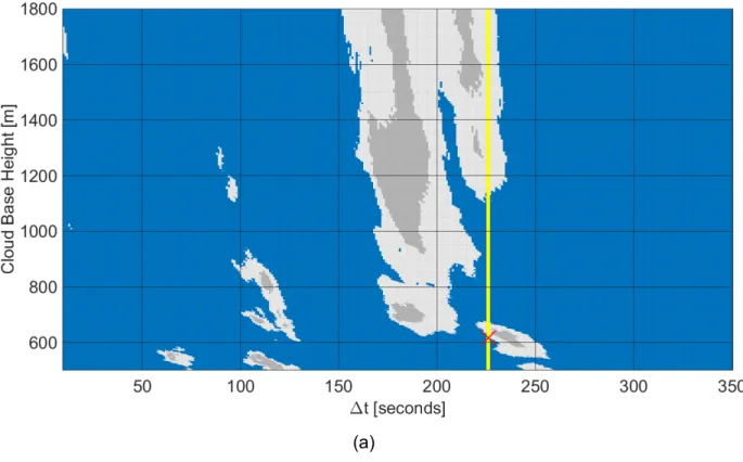
Figure 7 visualizes the 𝐻- ∆𝑡 map for the time window and GHI data corresponding to Figure 386

6. For illustration purposes, the CBH range is set to 500 m to 1800 m in 10 m increments and ∆𝑡 387

varies from 0 to 350 sec in 5 sec increments. The vertical yellow lines are placed at ∆𝑡 _¡¢ and 388

∆𝑡_{£ ¤¥}, indicating the respective station cloud travel times (as determined in Fig. 6). CBH 389

candidates are obtained from the 𝐻- ∆𝑡 map by searching for cloud condition transitions around 390

lines of constant ∆𝑡_$. The most commonly occurring CBH candidate across all stations is selected 391

as the CBH estimate. If two or more CBH candidates are equally common then they are averaged. 392

If none of the stations returns a CBH candidate, no CBH estimate is generated. Red crosses in 393

Fig. 7 indicate the CBH candidates are 620 m for BMSB, and 540 m and 660 m for EBU2. Thus, 394

the CBH candidates from the two stations are averaged to be 606 m. The concurrent ceilometer 395

reading at 12: 59: 00 LST indicates a single cloud layer at 610 m. 396

(b)

Figure 7: CBH versus arrival time (or 𝐻- ∆𝑡 map) for the initial time 𝑡$= 12: 56: 00 LST on May 19, 2014. Ramp events, indicated by the vertical yellow lines, were detected at ∆𝑡 = 226 s and ∆𝑡 = 319 s for the (a) BMSB and (b) EBU2 ground stations, respectively (see Figure 2 for locations and Figure 6 for ramp detection). Left-to-right transitions from clear to cloudy (i.e. down ramps) along the yellow line indicate CBH candidates (red cross). Blue, white, and grey colors represent clear sky, thin clouds, and thick clouds, respectively.

Note that the ∆𝑡 axis scales linearly with the cloud velocity, so uncertainty in 𝐮 contributes 397

directly to uncertainty in ∆𝑡. This and other potential errors in down ramp timing estimates (see 398

discussion in Section 5.2) justify extending the cloud condition transition search to a search 399

window of 60 seconds around lines of constant ∆𝑡_$. While this process induces more CBH 400

candidates, it reduces the times when no CBH estimate is output. 401

402

An alternate, more intuitive presentation of the 𝐻- ∆𝑡map is the cloud shadow distribution plan 403

view in Fig. 8, generated using the 𝑡$ cloud map advected at cloud velocity 𝐮 to time 𝑡$+ ∆𝑡. In

404

each subplot of Fig. 8, a shadow is just about to pass over the stations (note the shadow adjacent 405

to each red dot and the direction of cloud movement). The plan view gives the cloud shadow 406

distribution for all stations at a single (𝐻, ∆𝑡) pair, whereas the 𝐻- ∆𝑡 map gives the possible cloud 407

condition for a single station at a range of (𝐻, ∆𝑡). 408

409

(a)

(b)

Figure 8: Advected cloud shadow map generated from the sky image taken at 𝑡$= 12: 56: 00 LST on May 19, 2014 using arrival time of the down ramp of (a) ∆𝑡 ¡¢ = 226 s and (b) ∆𝑡£ ¤¥= 319 s and a

CBH of 606 m determined in Fig. 7. BMSB (a) and EBU2 (b) ground stations are shown as red filled squares. Empty squares represent the five other ground stations. The arrow indicates the cloud motion vector, showing the cloud shadows moving towards northeast. The arrow magnitude indicates the distance traveled by a cloud in 30 s. Blue, white, and grey colors represent clear sky, thin cloud, and thick cloud, respectively.

4.

Results

410

4.1

Median Filtering and Error Metrics

The non-uniform ceilometer measurements are first resampled to the TSC and GCSE time 412

steps through nearest neighbor interpolation. A sliding 15 minute median filter is then applied to 413

the raw output of TSC, GCSE, and the resampled ceilometer measurements. To quantify the 414

differences between the proposed methods and the ceilometer output, the mean bias difference 415

(MBD) and the root mean square difference (RMSD) were used: 416 417 MBD = 1 𝑵| (𝐻𝒏;+<57− 𝐻𝒏1567) 𝑵 𝒏zk , (12) 418 RMSD = -1 𝑵| (𝐻𝒏;+<57− 𝐻𝒏1567)¥ 𝑵 𝒏zk , (13) 419

where 𝑵 is the total number of data points, 𝐻_𝒏;+<57 _{is the CBH from the TSC and GCSE methods,}

420

and 𝐻_𝒏1567 _{is the corresponding ceilometer measurement at time index 𝒏. MBD and RMSD are}

421

divided by the daily average CBH measurement from ceilometer to obtain a normalized MBD 422

(nMBD) and normalized RMSD (nRMSD). Normalization provides a better comparison across days 423

(RMSD is expected to be proportional to the true cloud height), whereas the un-normalized metrics 424

give a better characterization of CBH accuracy for solar power forecasting. Periods with rain, 425

either falling or droplets remaining on the sky imager, were excluded from the evaluation since 426

neither ceilometer nor sky imager methods perform reliably under those conditions. Rainy periods 427

are shaded in yellow. 428

429

4.2

Evaluation over 30 Cloudy Days

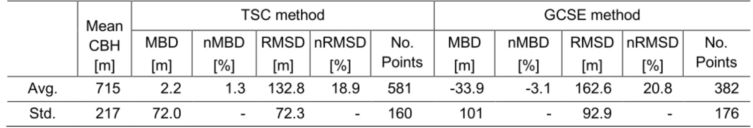
The performance for 30 days, spanning all seasons and multiple cloud types is given in Figure 431

9 and summarized in Table 2 (see Table A-1 in Appendix for complete comparison). 432

Stratocumulus and cumulus clouds were most common on the selected days. Only four of the 30 433

days had CBHs exceeding 1000 m, so the evaluation provided is predominantly for low cloud 434

conditions consistent with the dominant climatology of coastal Southern California. Overall, TSC 435

outperformed GCSE for this extended data set, with TSC achieving an average RMSD of 133 m 436

versus 163 m for GCSE. The standard deviation of daily RMSD for TSC was 72.3 m versus 92.9 437

m for GCSE, indicating the performance of TSC is more consistent across days. TSC had a small 438

positive bias, versus a small negative bias for GCSE. 439

The number of CBH values reported per day varies markedly between TSC and GCSE. GCSE 440

yields no result if there are no clouds detected that will shade the station. This will occur during 441

periods with sufficiently homogenous cloud conditions and specifically periods with clear or 442

overcast conditions along the cloud motion vector such that no CBH candidates are generated 443

for the available ground stations, i.e. there are no clouds within ∆𝑡$ ± 𝜎¯ for each station 𝑖 in the

444

𝐻- ∆𝑡 map. Additionally, GCSE cannot generate CBH if no down ramps are located. These 445

limitations cause GCSE to issue 34% less CBH than TSC averaged over 30 days. 446

447

448

Figure 9: Validation of cloud base height estimates for 30 days. Line styles distinguish error metrics, and line colors

449

differentiate TSC and GCSE methods, respectively. The number of raw measurements are displayed in black dots

450

(right y axis).

451 452

according to the number of data points. Ceilometer daily averages are reported as ‘Mean CBH’. Refer to Table A-1 in the Appendix for error metrics by day.

Mean CBH

[m]

TSC method GCSE method

MBD [m] nMBD [%] RMSD [m] nRMSD [%] No. Points MBD [m] nMBD [%] RMSD [m] nRMSD [%] No. Points Avg. 715 2.2 1.3 132.8 18.9 581 -33.9 -3.1 162.6 20.8 382 Std. 217 72.0 - 72.3 - 160 101 - 92.9 - 176 453

4.3

Comparison to NK14 on Select Days

Table 3 and Figure 10 present further validation against NK14 on three days. While it produces 455

scattered raw results, TSC captures the major CBH transition on all three days. In contrast, the 456

CBH estimates from GCSE are not as scattered likely because of the internal quality control that 457

requires CBH output consensus between stations. RMSD errors for TSC and NK14 are less than 458

300 m (RMSD) and 20% (nRMSD) averaged over the three days. GCSE, however, has RMSD and 459

nRMSD of over 400 m and 27%, respectively, performing consistently worse than the other two 460

methods. The MBD and nMBD show that the bias of GCSE is almost twice that of TSC for these 461

three days. Note that nRMSD seems higher for Dec 26 on both methods; however, the absolute 462

error on Dec 26 is not unusual and the large error can be attributed to the normalization by a 463

smaller CBH. NK14 beats both TSC and GCSE on all three days, though the performance of TSC 464

is close to that of NK14. 465

466

Table 3: Comparison of cloud base height estimates. Ceilometer daily averages are reported as ‘Mean CBH’. The average for each column (‘Avg.’) is weighted according to the number of data points in each day. Rainy periods are excluded.

Date

Mean CBH

[m]

TSC method GCSE method NK14: Stereographic MBD [m] nMBD [%] RMSD [m] nRMSD [%] MBD [m] nMBD [%] RMSD [m] nRMSD [%] RMSD [m] nRMSD [%] Dec 14 1814 88 4.9 291 16.0 -223 -12.3 394 21.7 262 14.3 Dec 26 1164 -128 -11.0 288 24.8 -323 -27.8 399 34.3 206 17.7 Dec 29 1625 -103 -6.3 299 18.4 169 10.4 440 27.1 272 16.8 Avg. 1534 -47.8 -4.0 293 19.5% -104.3 -8.3 413 27.4 246 16.3 467 468

(a)

(c)

Figure 10: Cloud base height comparison between the TSC (black dot), GCSE (green dot), and 2D stereographic method (red, Nguyen and Kleissl, 2014), and ceilometer measurements (green dashed) for (a) Dec 14, (b) Dec 26, (c) Dec 29, 2012. Yellow highlights show periods of rain that are ignored in the error calculation in Section 4.1.

469 470

5.

Discussion

5.1

TSC Performance

TSC computes the average correlation coefficient between 20 minutes of measured and 473

modeled GHI across several ground stations. Correlation coefficients are computed for a range 474

of CBH values, and the CBH corresponding to the maximum correlation is output. While the bias 475

of the method over 30 days is small at 1.3% nMBD, the random error is significant at 18.9% 476

nRMSD. Although this may seem high, it is within 3 percentage points of the stereographic method. 477

The following subsections highlight different factors affecting the performance of TSC method. 478

5.1.1

GHI Sampling and Correlation

Forty-one (41) samples are used to compute the correlation coefficients which are 480

subsequently averaged across stations. The 20 minute sample duration may be insufficient to 481

yield a reliable CBH estimate, but is chosen empirically to allow the method to be sufficiently 482

dynamic to track intra-hour changes in CBH. Increasing the time window may reduce the 483

estimator variance at the expense of being unable to react to rapid CBH changes. An alternative 484

to increasing the sample duration is to decrease the sampling (image capture) time step (i.e. 30 485

seconds) in this work. Beyond increasing the number of samples, treating the sensor network as 486

an array and applying array signal processing methods may provide a lower variance CBH 487

estimator. 488

5.1.2

Sensitivity of CBH to Correlation Coefficient

During certain periods, the variation of the correlation coefficients 𝑅₉ over all CBH candidates 490

was found to be small. For example, Figure 11 gives the mean correlation 𝑅9 (Eq. Error!

491

Reference source not found.) at different 𝐻₉ for a selected period. The maximum 𝑅₉ is very 492

similar to the minimum with 𝑅₉ ranging from 0.9 to 1. While the changes in 𝑅₉ are small relative to 493

its range, the relative changes in 𝐻₉ are considerable at 1050 m to 1700 m. In this case, due to 494

the small difference between the minimum and maximum correlation coefficient, the selected 𝐻₉ 495

may be determined by small and somewhat random fluctuations in 𝑅₉ which is not desirable 496

behavior for an accurate and robust CBH estimation algorithm. Small variations in the correlations 497

are caused by homogenous cloud cover (e.g. overcast condition) or a cloud projection that is 498

insensitive to CBH changes (e.g. collocated sky imagery and pyranometer). 499

Figure 11: Example of CBH estimates for the TSC method versus the ceilometer for a 45 minute period on Dec 29, 2012. The color of each symbol indicates the average correlation coefficient 𝑅9 (Eqs. Error!

Reference source not found. and Error! Reference source not found.) between the observed and simulated nowcast GHI from the set of stations. For each time step the CBH (y-axis) and its associated maximum 𝑅9 (filled circles) and minimum 𝑅9 (open hexagrams) are shown.

Moreover, larger imager to station distance can promote errors in the GHI time series from the sky imager. As indicated in Eq. (9 a larger pixel zenith angle (more distant station) results in cloud projection being more sensitive to CBH changes because the cloud projection error scales with 𝑡𝑎𝑛𝜃. In addition, the lower pixel resolution for the outer part of the sky image at larger pixel zenith angle can cause larger random errors in shadow projection at the ground station.

501

5.2

GCSE Performance

GCSE combines ramp detection with an analytic-geometric component derived from the sky 503

imager forecast. Down ramp events are detected for each ground station and associated cloud 504

edges are matched in each station's 𝐻- ∆𝑡 map. Since the construction of 𝐻- ∆𝑡 map is a matrix 505

indexing operation for an image, it takes less than a second to construct 𝐻- ∆𝑡 map on a typical 506

i5-powered workstation, making operational use feasible. 507

In terms of nRMSD, GCSE performed over 10 percentage points worse than the NK14 method 508

over the three days studied. In the more extensive 30 day comparison, GCSE improved 509

substantially with an nRMSD of 20.8%. For all error metrics, the GCSE performed worse than 510

TSC. This is in large part due to the modeling complexity and assumptions involved (see Section 511

5.3). 512

513

5.2.1

Down Ramp Start Time

An accurate down ramp start time from GHI observations is required for the GCSE to work 515

correctly. The method described in Section 3.2.2 is a reasonable approach if the ramp is 516

monotonically up or down. But in some cases ramps exhibit local extrema, causing the proposed 517

approach to misidentify the start time. 518

Figure 12 provides an example on Dec 26 with scattered cumulus clouds. Fig. 12a shows a 519

large down ramp with a complex kt time series: two local extrema are identified in the time series 520

maximum ramp points difference (Figure 5) at 12:23:21 LST (black dashed line) and 12:23:52 521

LST (green dashed line). The associated ramp event start times are determined at 12:23:26 LST 522

(black dot) and 12:23:47 LST (green dot), respectively, by searching within 5 second for a local 523

maximum in kt. While visual inspection suggests that the black dot is a reasonable ramp start 524

time, the kt variation around the two original local extrema is small, making identifying the start 525

time somewhat random. These small “pre-ramp” events are likely caused by the multiscale nature 526

of clouds and associated deformations around the cloud boundary. 527

The impact of this ambiguity in the local extremum is illustrated in Fig. 12b. The black dot in 528

(a) corresponds to black line (𝐻, ∆𝑡) = (775 m, 86 s) and the green dot in (a) corresponds to green 529

line (𝐻, ∆𝑡) = (625 m, 107 s) with ∆𝑡 = 0 at 12:22:00 LST. The two local extrema that are spaced 530

by 31 s cause a 150 m difference in CBH. In this case, the local extremum #1 is slightly greater 531

than #2, so it is selected per the procedure in Section 3.2.2 and the associated local maximum 532

(i.e. black dot) is used to determine the CBH candidate in Figure 12b. While in this case the final 533

selected CBH is closer to the ceilometer measurement of 866 m than the alternate, similar 534

ambiguities in local extremum and subsequent CBH variation were common in the analysis. 535

(a) (b)

Figure 12: Sensitivity of CBH to ramp start time and ambiguity in ramp start time estimation. (a) Two local extrema (dashed lines) are identified due to a non-monotic time series of kt (the dots show how following ramp detection each ramp start time is adjusted to the local maximum in kt within 5 sec). (b) 𝐻- ∆𝑡 map corresponding to (a) with ∆t = 0 sec at 12:22:00 LST. The vertical lines in (b) correspond to

the colored dots in (a). The actual CBH measurement from ceilometer is 866 m.

536

5.3

Other Modeling Errors Affecting CBH Estimation

Both TSC and GCSE rely on derived products generated in the USI forecast procedure that 538

apply simplifying assumptions and inject additional uncertainty into CBH estimation. Naturally, 539

since sky images are the key input to both methods, TSC and GCSE are not operational at night. 540

Cloud edges derived from sky imagery rely on the cloud decision process determining where 541

clouds "begin". The methods to detect cloud presence are generally accurate, but there is some 542

inherent uncertainty in a binary pixel classification as being-cloudy or cloud-free (Ghonima et al., 543

2012), particularly near cloud edges which may have a diffuse and blurred transition. This affects 544

both TSC and GCSE. 545

Another issue is that extensive cloud evaporation and formation can cause GCSE to fail 546

because the “frozen” cloud advection assumption is violated. Consider the case where a cloud 547

forms between time 𝑡_* when a sky image is taken, and the time when that cloud’s edge causes a 548

down ramp at time 𝑡_k. Another stable cloud that was present in the sky image at 𝑡_* causes a down 549

ramp at time 𝑡_¥ where 𝑡_¥ > 𝑡_k. Although the down ramp occurring at 𝑡_k is detectable in GHI data, 550

the cloud map generated from data at 𝑡_* only has the information of the cloud which passes at 𝑡_¥. 551

For TSC, this increases the separation between the measured and modeled GHI time series, 552

affecting correlation coefficients across the CBH grid search. The GCSE ramp detection algorithm 553

will return a ramp occurrence time of ∆𝑡_k= 𝑡_k− 𝑡_* which does not have a matching cloud edge in 554

the 𝐻- ∆𝑡 map. The 𝐻- ∆𝑡 map search process will yield the best available clear-cloudy transition 555

at ∆𝑡_k which is likely to be incorrect. 556

Besides, both methods are affected by overcast conditions with homogenous cloud cover. 557

The TSC method identifies concurrent cloud edge events using the correlation coefficient. If the 558

20 minute sample window does not contain any significant cloud-edge induced fluctuations, the 559

correlation coefficients are small and likely no CBH will be output. The GCSE method does not 560

provide CBH in overcast conditions either; while ramp detection may still be feasible due to 561

variability of cloud optical depth in overcast conditions, the cloud travel time cannot be estimated 562

from the binary 𝐻- ∆𝑡 map. Fortunately, in overcast or clear conditions the solar irradiance can be 563

predicted accurately without CBH because all stations are likely covered by the same sky 564

condition and receive similar irradiance. 565

Additionally, the pixel resolution for the outer part of the sky image at larger pixel zenith angle 566

is degraded, making the estimated cloud cover more uniform over the 20-minute comparison 567

interval. Any station whose shadow projection comes from these perimeter image sections will 568

lack detailed cloud structure. This less detailed cloud structure yields lower correlation for the 569

TSC, and larger errors in identifying the timing of sky condition changes for the GCSE. 570

Interestingly, for the GCSE, the forecast at the sky imager position is unaffected by CBH and thus 571

the forecast GHI does not suffer from CBH errors. 572

The temporal resolutions for TSC and GCSE differ: the TSC output rate is one sample per 30 573

seconds as set by the image capture frequency, but data availability may be less frequent due to 574

low correlation coefficients. The GCSE’s output rate depends on the existence of sufficient 575

variability in cloud cover, and the ability to find a consensus CBH candidate. For the dataset 576

presented here, GCSE outputs 34% less CBH samples than TSC, for an average of one GCSE 577

sample every 75 seconds. While this lower output rate is sufficient for short-term solar power 578

forecasting, it may be a limiting factor for other applications or in other sky conditions with less 579

cloud cover. The valid time of the CBH estimates also differs between methods: Since TSC 580

correlates the last 20 minutes of GHI data, the estimated CBH applies to those 20 minutes. While 581

GCSE utilizes only a single dominant down ramp in the GHI time series the CBH strictly applies 582

to that time instant only. 583

The cloud velocity estimation of the sky imager is actually an apparent cloud edge velocity, 584

which is a combination of cloud speeds due to advection along with cloud formation or evaporation 585

occurring from image to image. These cloud dynamics introduce real or apparent fluctuations in 586

cloud speed which negatively affects the performance of GCSE because construction of the 𝐻- ∆𝑡 587

map assumes that the cloud velocity remains constant over the CBH estimation interval (typically 588

10 minutes). TSC is insensitive to cloud speed variability as it does not employ a cloud advection 589

scheme. 590

Last, multiple cloud layers and cloud three-dimensionality (Mejia et al., 2018) can degrade the 591

performance because both methods operate under assumption of single-layered planar cloud 592

cover. 593

5.4

Number of Stations and Spatial Diversity

Geographic variations at the individual sites may affect both TSC and GCSE. For TSC, 595

averaging correlation coefficients at each CBH blurs potential station-to-station differences in 596

correlation coefficient due to real differences in CBH. For GCSE, station-to-station ramp timing 597

errors may cause inconsistent CBH candidates, preventing an accurate CBH estimate. The 598

current limitation of our setup was the availability of only six stations, four of which were located 599

within 600 m of each other resulting in more correlated GHI data and little diversity in perspectives. 600

A logical extension to this work is to examine the impact of adding additional ground stations. At 601

large solar installations, weather stations, reference cells, and individually metered inverters can 602

all be used to improve spatial distribution of stations. 603

6.

Conclusions and Future Work

604

The objective of this paper was to propose two methods for CBH estimation requiring a single 605

sky imager together with spatially distributed irradiance or power output measurements, providing 606

an alternative CBH estimation technique to direct, in-situ, or multi-camera approaches. These 607

new methods can serve as a low-cost alternative to ceilometers for sky imager based short-term 608

solar power forecasting in which the cloud height information is required (Chow et al., 2011; 609

Schmidt et al., 2016). 610

The TSC method, is comparatively simple and the more reliable of the two proposed methods. 611

The GCSE method relies on a complex stack of models: cloud detection, cloud velocity estimation, 612

cloud shadow forecasting, and down ramp detection. The construction of the 𝐻- ∆𝑡 map is a novel 613

feature of this work, and its utility is demonstrated for the purposes of cloud edge matching and 614

CBH estimation. Overall, the GCSE method performed slightly worse (1 percentage point larger 615

nRMSD) than the TSC method. For both methods, the nRMSD remained below 21% for all 30 616

days. On the other hand, the CBH estimate derived from a sky imager coupled with a cloud speed 617

sensor in our previous work (Wang et al., 2016) yielded better accuracy (17% nRMSD) on a 618

different set of 30 days, owing partially to the strict filtering of the raw cloud speed measurement. 619

Future efforts will involve improving both sky imager cloud detection and cloud velocity 620

estimation, which will also benefit solar power forecasting with a sky imager. Chow et al. (2015) 621

proposed optical flow to enable detection of multiple cloud layers as well as their respective cloud 622

pixel speeds, which is an improvement to the cross-correlation velocity estimation method used 623

in this work. Adding more and more distributed ground stations will also help improve the 624

robustness of the methods. Finally, validation under different meteorological conditions more 625

relevant to continental climates would further substantiate the general applicability of the methods. 626

627 628

Appendix

629

Table A-1: Comparison of cloud base height estimates between TSC and GCSE methods for 30 days. Ceilometer daily averages are reported as ‘Mean CBH’.

Date

Mean CBH

[m]

TSC method GCSE method

MBD [m] nMBD [%] RMSD [m] nRMSD [%] No. Points MBD [m] nMBD [%] RMSD [m] nRMSD [%] No. Points 09/20/13 613 -90.5 -14.8 123.6 20.2 616 -104.7 -17.1 129.9 21.2 157 09/21/13 695 40.6 5.8 109.9 15.8 752 45.3 6.5 124.4 17.9 362 09/22/13 618 137.0 22.2 144.5 23.4 750 129.0 20.9 138.9 22.5 217 10/02/13 598 -14.5 -2.4 66.7 11.2 337 -109.9 -18.4 161.1 26.9 408 02/04/14 1110 -41.5 -3.7 294.4 26.5 410 -161.6 -14.6 296.0 26.7 712 02/09/14 747 32.7 4.4 118.9 15.9 606 -51.1 -6.8 156.8 21.0 473 02/10/14 648 88.3 13.6 135.0 20.8 822 76.5 11.8 118.2 18.2 291 03/22/14 1116 -241.4 -21.6 365.9 32.8 424 -389.6 -34.9 444.7 39.9 416 03/23/14 657 -27.7 -4.2 122.3 18.6 696 -40.8 -6.2 118.6 18.1 219 03/25/14 651 -40.0 -6.1 282.6 43.4 750 -33.7 -5.2 258.7 39.7 141 03/27/14 971 43.5 4.5 268.0 27.6 504 94.9 9.8 315.7 32.5 646 05/20/14 783 33.1 4.2 162.7 20.8 460 -98.3 -12.5 197.7 25.2 679 06/10/14 633 -18.6 -3.0 101.7 16.6 552 -81.6 -12.9 120.8 19.1 283 04/20/15 662 -65.9 -10.0 107.2 16.2 531 -85.1 -12.9 110.2 16.6 209 05/21/15 1263 -65.6 -5.2 288.8 22.9 285 -73.8 -5.8 324.0 25.6 213 04/12/16 460 58.6 12.7 89.4 19.4 471 62.1 13.5 108.9 23.7 389 04/22/16 485 42.7 8.8 89.4 18.4 563 -0.9 -0.2 87.6 18.1 404 04/25/16 998 -2.8 -0.3 147.4 14.8 760 -11.1 -1.1 145.7 14.6 847 05/21/16 1004 51.9 5.2 97.1 9.7 525 -23.5 -2.3 148.4 14.8 507 05/23/16 916 61.9 6.8 124.4 13.6 361 69.7 7.6 128.4 14.0 411 05/26/16 771 99.2 12.9 124.3 16.1 309 31.3 4.1 212.4 27.5 342 07/17/16 409 73.5 18.0 97.1 23.7 672 70.9 17.3 93.3 22.8 266 08/11/16 555 17.4 3.1 93.4 16.8 374 -15.7 -2.8 82.9 14.9 610 08/26/16 725 -49.0 -6.8 82.5 11.4 773 -60.0 -8.3 85.3 11.8 323 08/28/16 376 52.8 14.0 64.5 17.2 744 38.4 10.2 56.0 14.9 520 09/02/16 514 -46.6 -9.1 62.9 12.2 614 -59.3 -11.5 68.4 13.3 280 09/08/16 603 -42.5 -7.0 80.6 13.4 605 -53.5 -8.9 83.4 13.8 253 09/09/16 469 18.1 3.9 41.2 8.8 654 19.5 4.2 40.0 8.5 278 09/12/16 714 27.3 3.8 102.7 14.4 699 26.3 3.7 93.2 13.1 237 10/12/16 689 -118.9 -17.3 156.4 22.7 805 -134.4 -19.5 171.5 24.9 377 630