Modeling IP traffic using the batch Markovian arrival process

Alexander Klemm, Christoph Lindemann*, and Marco Lohmann University of Dortmund

Department of Computer Science August-Schmidt-Str. 12 44227 Dortmund, Germany

[email protected], [email protected], [email protected] http://www4.cs.uni-dortmund.de/~Lindemann/

Tel: (+49231) 755-2410 Fax: (+49231) 755-2417

Abstract

In this paper, we show how to utilize the expectation-maximization (EM) algorithm for efficient and numerical stable parameter estimation of the batch Markovian arrival process (BMAP). In fact, effective computational formulas for the E-step of the EM algorithm are presented, which utilize the well-known randomization technique and a stable calculation of Poisson jump probabilities. Moreover, we identify the BMAP as an analytically tractable model of choice for aggregated traffic modeling of IP networks. The key idea of this aggregated traffic model lies in customizing the BMAP such that different lengths of IP packets are represented by rewards of the BMAP. Using measured traffic data, a comparative study with the MMPP and the Poisson process illustrates the effectiveness of the customized BMAP for IP traffic modeling by visual inspection of sample paths over several time scales, by presenting important statistical properties as well as by investigations of queuing behavior.

Key words:

Parameter estimation,

numerical transient analysis of Markov chains, analytical/numerical models of aggregated IP traffic, EM algorithm.

* _{Corresponding author}

1 Introduction

Traffic characterization and modeling constitute important steps towards understanding and solving performance-related problems in future IP networks. The central idea of traffic modeling lies in constructing models that capture the most important statistical properties of the underlying measured trace data [2]. For IP traffic, important statistical properties are

burstiness and self-similarity. Intuitively, this means that measured IP traffic shows noticeable

sustained periods with arrivals above the mean (i.e., bursts) over a wide range of different time scales [21]. Aggregated traffic models capture the entire traffic stream without explicitly considering individual traffic sources, e.g. the traffic originated by individual users. The problem of accurately capturing these properties in aggregated traffic models has been solved for non-analytically tractable models but is still subject of current research interest for analytically tractable models. Non-analytically tractable models, e.g. fractional Gaussian noise (fGN) and fractional autoregressive integrated moving average (fARIMA), naturally capture burstiness as well as self-similarity [10]. Various research papers have subjected these models, e.g. Ledesma and Liu reported the effective construction of fGN in [12].

For analytically tractable models, e.g. the Markov-modulated Poisson process (MMPP, [7]), recent work has been proposed that utilizes the MMPP in order to mimic self-similar behavior [1], [22]. Skelly, Schwartz, and Dixit [16] utilized the MMPP for video traffic modeling. They described a simple and efficient method for parameter estimation of a general MMPP based on the match of the marginal distribution of the arrival rate. The class of batch Markovian arrival process (BMAP, [13]) includes the well known Poisson-process, MMPP, and Markovian arrival process (MAP, [13]) as special cases and additionally associates rewards (i.e., batch sizes of arrivals) to arrival times. However, due to the addition of rewards the BMAP provides a more comprehensive tool for representing IP traffic than the MMPP or the MAP, while still being analytically tractable.

The challenge for employing BMAPs to model IP traffic constitutes the proper parameter estimation for this arrival process from the given trace data. In fact, measured trace data does not contain all statistical properties required for the unique specification of a corresponding BMAP. Due to this incomplete data, the parameters for a BMAP cannot be properly estimated by standard statistical techniques, e.g. moment matching. Dempster, Laird, and Rubin introduced the expectation-maximization (EM) algorithm [5] for computing maximum likelihood estimates from incomplete data. Based on this work, Asmussen proposed an EM algorithm for PH renewal processes [3]. Deng and Mark introduced a first approach for adapting the EM algorithm to an MMPP [6]. Ryden tailored the EM algorithm for the MMPP and developed an implementation [15]. To the best of our knowledge, tailoring the EM algorithm for BMAPs, developing a numerical stable implementation and utilizing the BMAP for traffic modeling is an open research problem.

In this paper, we introduce an efficient and numerical stable method for estimating the parameters of a BMAP with the EM algorithm. We show how the randomization technique [9], [14], [17] and a stable calculation of Poisson jump probabilities [8] can effectively be utilized for the computation of the time-dependent conditional expectation of a continuous-time Markov chain (CTMC) required by the E-step of the EM algorithm. In fact, we present efficient computational formulas for the E-step of the EM algorithm and show how to utilize the EM algorithm for the effective parameter estimation of BMAPs. Based on these methodological results, we introduce a framework for traffic modeling of aggregated IP traffic utilizing the BMAP, which both is analytically tractable and closely captures the statistics of the measured traffic data. The key idea of this aggregated traffic model lies in customizing the batch Markovian arrival process such that different lengths of IP packets are represented by rewards, i.e., batch sizes of arrivals, of the BMAP. In order to show the advantage of the BMAP modeling approach over other widely used analytically tractable models, we compare the customized BMAP with the MMPP and the Poisson process by means of visual inspection of sample paths over four different time scales, by presenting important statistical properties, by formal analysis of traffic burstiness using R/S statistics, and by queuing system analysis.

This paper is organized as follows. To make the paper self-contained, Section 2 recalls the definition and properties of the BMAP and the randomization technique for numerical transient analysis of Markov chains. Section 3 provides a primer to the EM algorithm and presents effective computational formulas for the expectation step (E-step) and the maximization step (M-step) tailored to the BMAP. In Section 4, we present a framework for traffic modeling of aggregated IP traffic utilizing the BMAP. A comparative study illustrates the effectiveness of the proposed parameter estimation procedure and the accuracy of the proposed traffic model. Finally, concluding remarks are given.

2 Mathematical

Background

2.1 The Batch Markovian Arrival Process

The batch Markovian arrival process (BMAP) belongs to the class of Markov renewal

processes. Consider a continuous-time Markov chain (CTMC, [13]) with

(

N+1

)

states

{

0,1,…, N

}

, where the states in

{

1, 2 ,…, N

}

are transient and 0 is absorbing. Moreover, π

denotes the initial state probability vector of the CTMC. Based on this governing CTMC, the BMAP can be constructed as follows: The CTMC evolves until an absorption in state 0

occurs. The chain is then instantaneously restarted in one of the transient states

{

1, 2 ,…, N

}

.

When restarting the BMAP after absorption in a transient state j, the probability for selecting state j is allowed to depend on state i from which absorption has occurred. Thus, the distribution of the next arrival may depend on the previous history. Furthermore, there may

exist multiple paths between two states i and j corresponding to different rewards, i.e., batch sizes of arrivals. Due to the addition of rewards the BMAP provides a more comprehensive model for representing IP traffic than the MMPP and the MAP, while still being analytically tractable.

Formally, assume the BMAP is in a transient state i for an exponentially distributed time

with rate λi. When the sojourn time has elapsed, there are

(

M +1

)

possible cases for state

transitions: With probability P

( )

m _{i j,} the BMAP enters the absorbing state 0 and an arrival of

batch size m occurs. Then, the process is instantaneously restarted in state j. Note that the

selection of state j (1 ≤ j ≤ N) and batch size m (1 ≤ m ≤ M) is uniquely determined by

( )

m i j,

P . On the other hand, with probability P

( )

0 _{i j,} the BMAP enters another transient state

j, j≠i, without arrivals. We can define D

( )

0 _{i j,} = λ ⋅i P

( )

0 _{i j,} for i≠ j, D

( )

0 _{i i,} = −λi, and

( )

m i j, = λ ⋅i

( )

m i j,

D P . Here, D

( )

0 defines the rate matrix of transitions without arrivals,

whereas the matrices D

( )

m define rate matrices of transitions with arrivals of batch size m

(1 ≤ m ≤ M). Summing up D

( )

0 and D

( )

m (1 ≤ m ≤ M) leads to

( )

0 M_m1

( )

m

=

= +

∑

D D D ,

where D is the infinitesimal generator matrix of the CTMC underlying the BMAP.

Furthermore, the matrix fm

( )

t of probability density functions (pdf) defines probability laws

for state changes in the CTMC from i to j with an arrival of batch size m at time t. The matrix

of complementary cumulative distribution functions (ccdf) Fc

( )

t defines conditional

probabilities that given the CTMC is in state i the chain will reside in state j at time t without arrivals until time t. The matrices fm

( )

t and

( )

c t F are given by

( )

( )0

_{( )}

e t m t = ⋅ m D f D and Fc

( )

t =eD( )0t. (1)

Recall, that the key idea of considering both the interarrival-times and packet lengths relies in regarding the packet lengths as the rewards of the BMAP. In Section 3, we introduce a computational efficient and numerical robust EM (expectation maximization) algorithm [5]

for the parameter estimation process of BMAPs, i.e., estimation of the parameter set φ

comprising the probability vector π and the transition rate matrices D

( )

0 ,…,D

( )

M . Based

on this parameter estimation, such a customized BMAP constitutes an aggregated IP traffic model considering both packet interarrival-times and packet lengths.

2.2 The Randomization Technique

Randomization (also called uniformization or Jensen's method [9], [14], [14a]) has proven to be an effective numerical method for computing transient measures of CTMCs involving matrix exponentials as introduced in Eq. (1). Reibman and Trivedi showed that randomization constitutes the method of choice for non-stiff and mildly stiff CTMCs. For transient analysis of stiff CTMCs, the implicit Runge-Kutta method can effectively be employed [14]. Applying the randomization technique to a continuous-time Markov chain with generator matrix Q of dimension N, a scalar 1 , 1.02 max i N i i q ≤ ≤ = ⋅ Q and a matrix A

1

q

= +

A Q I (2)

are defined. Scaling the maximum diagonal element q by the factor 1.02 ensures that the discrete-time Markov chain with generator A is aperiodic. Since negative entries of the matrix

Q are restricted to its diagonal, all entries of the matrix A are nonnegative. Rewriting equation

(2) yields Q=Aq−Iq and the matrix exponential eQt can be expressed as

eQt =eAqt⋅e−qt. (3)

Using the truncated series expansion of the matrix exponential and equation (3), the transient

probability vector π_t can be calculated by

( ) (

)

( , ) ( , ) 0 0 ( , ) ( , ) ( ) e e ; ! n R qt R qt t n qt t n L qt n L qt qt n n qt n ε ε − = ε = ε = ⋅ Q ≅

∑

⋅ ⋅ ⋅ =

∑

⋅β A π π π Φ , (4)

where L qt

(

,ε

)

and R qt

(

,ε

)

denote the left and right truncation points for a given error

tolerance ε, respectively.

In Eq. (4), Φ

( )

n denotes the state probability vector of the discrete-time Markov chain

with transition probability matrix A at step n. The term β

(

n qt;

)

denotes the probability mass

function of the Poisson distribution with parameter qt at n. According to Eq. (4), the

computation of the transient probability vector π_t of the continuous-time Markov chain is

reduced to the computation of the transient probability vector Φ

( )

n of a discrete-time

Markov chain with probability matrix A and appropriate Poisson probabilities. The function

( )

n

Φ can be efficiently computed by recursive vector-matrix multiplications [9] by

( )

0 = 0

Φ π and Φ

(

n+ =1

)

Φ

( )

n ⋅A. (5)

Since the probability mass function of the Poisson distribution thins for growing qt, round-off errors for large qt may affect the computation of Poisson probabilities. Thus, the randomization technique is enhanced by a stable calculation of Poisson probabilities proposed

by Fox and Glynn [8]. Given an error tolerance ε, the computational complexity of a

dense/sparse implementation of the randomization method is given by O N

(

2⋅qt

)

and

(

)

O η⋅qt , respectively, where η denotes the number of nonzero entries in the generator

matrix Q. Furthermore, the randomization technique is an efficient tool for calculating the

conditional expectation of the state probability vector of a CTMC in a time interval (0, ]t

3 The EM Algorithm for the BMAP

3.1 Fundamentals of the EM Algorithm

The EM algorithm [5] implements maximum likelihood estimation in case of incomplete data. Such incomplete data can be thought of as partial observations of a larger experiment. In fact, for a BMAP only arrivals times and batch sizes of arrivals, e.g. arrival times of IP packets and their packet lengths, are observable. All state changes in the governing CTMC not hitting the absorbing state are not observable and, thus, cannot be derived from measured trace data.

Formally, suppose that y is the observable part of a considered experiment. This experiment can be described completely by y and the non-observable data x denoted as the

missing data. Let L

( )

φ, y be the likelihood of a parameter set φ given the observation y and

let Lc

(

φ, ,x y

)

be the so-called complete likelihood of the parameter set φ including the

missing data x. Assume y=

{

(

t b₁, ₁

) (

, t b₂, ₂

)

,…,

(

t b_n, _n

)

}

is the observed sequence of interarrival times t and the corresponding batch sizes _k b . Define _k ∆ = −t_k t_k t_k−1 for 1 ≤ k ≤ n.

Then, the likelihood of a BMAP with parameter set φ is given by:

( )

( )

1 , k n b k k t = = ⋅

∏

∆ ⋅ y f 1 φ π L (6)

Recall that, in Eq. (6), π denotes the initial state probability vector of the CTMC,

( )

k

b t f

defines the matrix of probability density functions, and φ is a specific parameter set for the

BMAP comprising π and the transition rate matrices D

( )

0 ,…,D

( )

M . The vector 1

represents a vector of appropriate dimension comprising 1s in each entry. Note, that the (logarithm of the) likelihood measures the quality of the estimated parameter set [5].

The EM algorithm iteratively determines estimates of the missing parameter set φ of the

BMAP. Denote by φ

( )

r the parameter set calculated in the r-th iteration of the EM

algorithm. φ

( )

r comprises π

( )

r and D

( )

0,r ,…,D

(

M r,

)

, which denote the initial state probability vector as well as the transition rate matrices in the r-th iteration, respectively. We

denote further by P_φ and E_φ the conditional probability and the conditional expectation given

the estimate φ, respectively. As shown in [5], the estimate

( )

(

(

)

)

{

}

ˆ _{arg max log} c _{, ,}

r

= _{φ φ} x y y

φ E L φ , for r =0,1, 2,…, (7)

satisfies L

( )

φˆ,y ≥L

(

φ

( )

r ,y

)

and φ

(

r+ =1

)

φˆ is the estimate for the parameter set

determined in the

(

r+1

)

-th step of the algorithm. This iterative procedure is repeated until a

predefined maximum number of iterations is reached or until some convergence criteria

holds, which can be, for instance, that each component of φ

( )

r and φ

(

r+1

)

differs only up

to a predefined ε, respectively. The computation of the conditional expectation in (7) is called

the E-step whereas the derivation of the maximum in (7) constitutes the M-step of the EM

algorithm. As described in [15], the likelihood L

( )

φ, y is highly non-linear in φ and is

often be computed in closed form. This is the main reason for the widespread use of the EM algorithm. A further advantage of the EM algorithm over other maximum likelihood methods lies in the good convergence behavior of the iterative scheme regardless of the initial estimate

( )

0

φ .

Already for the MMPP, the problem with the practical applicability of the EM algorithm for parameter estimation lies in the stable numerical computation of matrix exponentials as

specified in Eq. (1). Ryden [15] proposed a diagonalization method to compute eQt, but this

approach relies on the diagonalization property of the matrix Q. It is known that decomposition techniques like diagonalization are in general not stable numerical methods for computing matrix exponentials [9]. In the next section, we show how to employ the randomization technique enhanced by a stable calculation of Poisson probabilities for the numerical computation of the matrix exponentials of Eq. (1) for the BMAP.

3.2 Effective

Computational Formulas for the BMAP

Recall that the observed data in a BMAP is

{

(

t b₁, ₁

) (

, t b₂, ₂

)

,…,

(

t b_n, _n

)

}

. The generator of the

CTMC

{

X t

( )

:t≥0

}

underlying the BMAP constitutes the missing data. We assume that

( )

N t is the counting process of the batch sizes for arrivals. Let

{

t_k:1≤ ≤k n

}

be the sequence

of arrival times. Without loss of generality, we assume t₀ =0 and t_n =T. Considering the

likelihood estimates of the EM algorithm introduced above, we show in the following how to maximize the likelihood for the parameter set of a BMAP.

First of all, we have to define the complete likelihood of the BMAP using the observed

data y and the non-observable data x. Let m k be the number of transient states entered

( )

during the k-th interarrival-time. Moreover, let i k and _l

( )

s k denote the l-th transient state _l

( )

and the sojourn time in the l-th transient state during the k-th interarrival-time, respectively. Then the complete likelihood of the BMAP is given by

(

)

( ) ( ) ( )

( )

( ) ( ) ( ) ( )( ) ( ) ( ) ( )( )

_{( )}

( )( ) ( ) 0 1 0 1 (1) _, 1 0 , 1 , , i kl l 0 l l l i_{m k} k m k m k m k m k n s k c i i k i k i k k l s k k i k i k i k e e b + − −λ ⋅ = = −λ ⋅ + = × λ ⋅ ⋅ ×λ ⋅ ⋅

∏ ∏

x y P P φ π L , (8)

where P

( )

m and λ_i are defined as in Section 2, ( )

( )

0 m k

j k

j= s k = ∆t

∑

, and b is the batch size of _k

the k-th arrival. The first term of the right hand side of Eq. (8) specifies the probability of

starting the CTMC in state i₀

( )

1 . For each arrival epoch of the BMAP, the second term

describes the transient trajectory up to a state i_{m k( )}

( )

k from which absorption occurs. The last

portion of Eq. (8) represents the transition from the transient state i_{m k( )}

( )

k to the absorbing

state 0 and the restarting of the process in state i k₀

(

+1

)

with an arrival of batch size b . _k

Recall that P

( )

m _{i j,} is the probability, given the chain is in state i, the process enters the

In order to simplify the notation in the estimation step, we define the sufficient statistics T,

( )

1 , ,

( )

M

A … A and s as follows. For 1 ≤ i, j ≤ N and i≠ j we define Ti j, as:

( )

( )

( )

( )

{

}

, # 0 , , , i j = t ≤ ≤t T X t− =i X t = j N t =N t− T (9) , i j

T is the number of transient state transitions from state i to state j without an arrival. For

1 ≤ m ≤ M and 1 ≤ i, j ≤ N we define A

( )

m _{i j,} as:

( )

m i j, =#

{

tk1≤ ≤k n X t,

( )

k − =i X t,

( )

k = j N t,

( )

k =N t

( )

k− +m

}

A (10)

( )

m i j,

A is the number of absorbing state transitions from state i to state j with an arrival of

batch size m at arrival times t . Finally, for 1 k ≤ i ≤ N we define s as: i

( )

(

)

0 T

i =

∫

X t =i dt

s I , where I

( )

⋅ is the indicator function. (11)

i

s captures the total time the CTMC resides in state i.

The key idea of these sufficient statistics is to capture the complete likelihood expression in a more intuitive fashion. Typically, the sufficient statistics can be determined by numerically tractable characteristics of the CTMC. Applying some calculus, these sufficient statistics can easily be used to rewrite and simplify the expression of the complete likelihood in Eq. (8). That is:

(

)

( ( )0 ) ( )0 ,

_{( )}

,

_{( )}

( ), , , 1 1 1 1, 1 1 1 , , i i i 0 i j i j N N N N M N N s m X i c i _{i j i j} i i i j j i m i j e ⋅ m = = = = = ≠ = = = =

∏

⋅

∏

D ⋅

∏ ∏

T ⋅

∏∏∏

A x y D D φ πI L (12)

Intuitively, the second product of Eq. (12) symbolizes the sojourn time of the CTMC for each state i. The third product of Eq. (12) captures the behavior for all transient state transitions between states i and j. Similarly, the last product of Eq. (12) represents the absorbing state transitions between states i and j with arrivals of batch size m.

When adopting (7) to the considered case of a BMAP, we have to recognize that

(

) (

)

(

)

{

t b1, 1 , t b2, 2 , , t bn, n

}

=

y … is completely characterized by the counting process N t( )

introduced above. This leads directly to Eq. (13) with the following abbreviations (14) to (17)

for ease of notation. In Eq. (13), the maximization ˆπ_i of π_i is already given in a natural way.

Furthermore, it can be shown that using the definition of a BMAP and appropriate partial differentiation, Eq. (13) is maximized by Eq. (18). Additionally to the maximization by partial differentiation, each of the expressions in Eq. (18) utilizes the maximized sufficient statistics (14) to (17) in a very intuitive manner. For example, Dˆ 0

( )

_{i j,} is the ratio of the total number of transient state transitions between states i and j and the total time spent in state i.

The expressions (13) to (17) in Figure 1 represent the E-step of the EM algorithm while the expressions in Figure 2 represent the M-Step of the EM algorithm. For ease of notation, we

define L( )k for k=0,…,n, as L(0)=π

( )

r and ( ) ( 1)

( )

k

b k

k = k− ⋅ ∆t

E-step: ( )

{

(

) ( )

}

( )

, ,

( )

,

( )

,

( )

, 1 1 1 1, 1 1 1 log , , , 0 ˆ ˆ ˆ

ˆ log 0 log 0 log

c r N N N N M N N i i i i i i j i j i j i j i i i j j i m i j N u u T m m = = = = ≠ = = = ≤ ≤ =

∑

⋅ +

∑

⋅ +

∑ ∑

⋅ +

∑∑∑

⋅ x y D s T D A D φ φ π π E L (13) where: ( )

{

( )

( )

}

ˆi = φr X 0 =i N u ,0≤ ≤u T π P . (14) ( )

{

( )

}

( )

(

( )

( )

)

0 ˆ ,0 , 0 T i = r s N ui ≤ ≤u T =

∫

r X t =i N u ≤ ≤u T dt s E_φ P_φ . (15) ( )

{

( )

( )

( )

( ) ( )

}

, 0 ˆ _{, , , 0} T i j =

∫

r X t− =i X t = j N t =N t− N u ≤ ≤u T dt T P_φ . (16)

( )

, _{( )}

{

( )

( )

( )

( )

( )

}

1 ˆ n _{, , , 0} k k k k r i j k m X t i X t j N t N t m N u u T = =

∑

− = = = − + ≤ ≤ A P_φ . (17)

Figure 1. E-step for parameter estimation of BMAPs

M-step:

( )

( )

(

( )

)

ˆ_i = _i r ⋅ ⋅1 R_i 1 r ,y π π L φ , for i=1,…,N.

( )

, , ˆ ₀ ˆ _ˆ i j i i j = D T s and ˆ

( )

_, ˆ

( )

_, ˆ_i i j i j m = m D A s , for i j, =1,…,N . (18)

( )

,

( )

,

( )

, 1, 1 1 ˆ ₀ N ˆ ₀ M N ˆ i i i j i j j j i m j m = ≠ = = = −

∑

−

∑∑

D D D , for i=1,…,N.

Figure 2. M-step for parameter estimation of BMAPs

fashion, for k = +n 1,…,1 R( )k is defined as R(n+ =1) 1 and ( )

( )

( 1)

k

b k

k = ∆ ⋅t k+

R f R . Let

i

1 and 1Ti denote the i-th unity column and row vector, respectively. The integrals over

matrix exponentials of Eqs. (15) and (16) can be transformed to Eq. (19) by means of probability laws.

(

) (

)

(

) (

)

1 1 1 1 k k k t c T k i j b k t k t t t t k dt − − − ⋅ − ⋅ ⋅ ⋅ − ⋅ +

∫

L F 1 1 f R (19)

These transformations as well as the detailed evaluation of Eqs. (14) and (17) are given in Appendix A and B, respectively. In Figure 3, we present the resulting expressions in algorithmic fashion. For efficient and reliable calculation of the integral over matrix exponentials of Eq. (19), we have derived effective computational formulas based on the

randomization technique. Appropriately adopting the limits and substituting the matrix exponentials of Eq. (19) by its series expansion yields

( ) ( )

( ) (

(

)

)

( ) 0 0 0 ! ! k k n m t k q t t qt k k m n q t t qt a m e b n e dt m n ∆ _{∞ ∞} − ∆ − − = = ∆ − ⋅ ⋅ ⋅ ⋅ ⋅

∑

∑

∫

, (20) where ak

( )

m =L

(

k− ⋅1

)

Am⋅1 and i

( )

_k

(

1

)

T n k j b

b n = ⋅1 A ⋅D ⋅R k+ . Applying some calculus

as well as simple integration rules (also given in Appendix A) and the truncated series expansion according to Eq. (4) leads to

( ) ( )

(

)

( ,) ( ,) 1 1; k k k k k L q t m n R q t a m b n m n q t q ∆ ε ≤ + ≤ ∆ ε ⋅ ⋅ ⋅β + + ∆

∑

, (21)

which can be efficiently and reliable calculated by means of the randomization technique and a stable calculation of Poisson probabilities [8]. Furthermore, we adopted the scaling procedure proposed in [15] for calculating the sufficient statistics T , ˆ_{i j,} Aˆ

( )

1 _{i j,} ,…,Aˆ

( )

M _{i j,} ,

ˆ_i

s , ˆπ_i, and the likelihood estimate L(φ

( )

r y, ). This scaling procedure is necessary because these quantities can take extremely small or extremely large values.

3.3 Efficient

Implementation

Figure 3 presents an iterative scheme for the implementation of the EM algorithm using the

forward-backward (Baum-Welch) method [15]. As shown in the appendix, the detailed

expressions of the maximized sufficient statistics ˆs and i T in Eqs. (26) and (27) reveal ˆi j,

strong similarities. Thus, the computation of ˆs can be performed by means of i T without ˆi j,

additional effort (see Figure 3, M-Step). Let max max

{ }

k

k

t = t . Assuming M <<n and λ <<n,

the computational complexity of a careful and efficient implementation of the E-Step and

M-Step is given by O n q t

(

⋅ ⋅ max⋅N2

)

for each iteration. Note, that this is the worst-case

computational complexity, where the randomization technique would have been always applied for q t⋅ max.

The initial parameter set φ

( )

0 can be determined by different approaches including simple

random initialization, precondition according to moment matching methods, and heuristic

initialization. All these approaches provide the common property that zero entries in φ

( )

0 are

preserved in the corresponding elements of the successive estimates φ

( )

r . This property

enables the estimation of specialized BMAPs, e.g. MAPs or MMPPs. For random

initialization, a set of initial estimates is generated randomly. Assuming λ <<n, the

likelihood of each estimate is evaluated with computation complexity O n

(

⋅log

(

q t⋅ max

)

⋅N2

)

and φ

( )

0 is set to the estimate that results in the maximum likelihood of these estimates.

Again, this denotes the worst-case computational complexity. For a discussion of initialization methods, we refer to [15]. In most cases, different initial estimates just result in a slightly different number of iterations in the scheme (7) required by the EM algorithm, whereas the quality of different estimated parameter sets is very similarly. As shown in

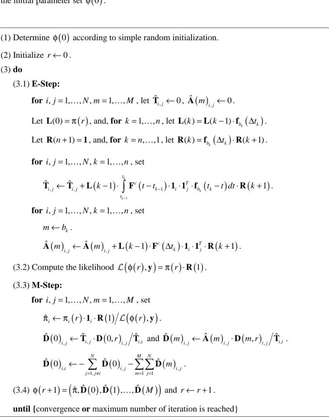
Section 4, the implementation of the EM algorithm based on the computational formulas presented here requires for each iteration only a few seconds of CPU time on a modern PC for considerable large trace files. Thus, we employ simple random initialization for determining the initial parameter set φ

( )

0 .

(1) Determine φ

( )

0 according to simple random initialization.

(2) Initialize r←0. (3) do (3.1) E-Step: for i j, =1,…,N m, =1,…,M , let Tˆ_{i j,} ←0,

( )

, ˆ ₀ i j m ← A .

Let L(0)=π

( )

r , and, for k=1,…,n, let ( ) ( 1)

( )

k

b k

k = k− ⋅ ∆t

L L f .

Let R(n+ =1) 1, and, for k =n,…,1, let ( )

( )

( 1)

k b k k = ∆ ⋅t k+ R f R . for i j, =1,…,N k, =1,…,n, set

(

)

(

)

(

)

(

)

1 , , 1 ˆ ˆ _{1 1} k k k t c T i j i j k i j b k t k t t t t dt k − − ← + − ⋅

∫

− ⋅ ⋅ ⋅ − ⋅ + T T L F 1 1 f R . for i j, =1,…,N k, =1,…,n, set m←b_k. Aˆ

( )

m _{i j,} ←Aˆ

( )

m _{i j,} +L

(

k− ⋅1

) ( )

Fc ∆ ⋅ ⋅ ⋅tk 1 1i Tj R

(

k+1

)

. (3.2) Compute the likelihood L

(

φ

( )

r ,y

)

=π

( ) ( )

r ⋅R 1 .

(3.3) M-Step: for i j, =1,…,N m, =1,…,M , set πˆ_i←π_i

( )

r ⋅ ⋅1 R_i

( )

1 L

(

φ

( )

r ,y

)

.

( )

_,

( )

_, , , ˆ ₀ ˆ _0, ˆ i j i i i j ← ⋅ r i j D T D T and

( )

( )

( )

_, , , , ˆ ˆ _, ˆ i i i j i j i j m ← m ⋅ m r D A D T .

( )

_,

( )

_,

( )

_, 1, 1 1 ˆ ₀ N ˆ ₀ M N ˆ i i i j i j j j i m j m = ≠ = = ← −

∑

−

∑∑

D D D . (3.4) φ

(

r+ =1

)

(

πˆ,Dˆ

( ) ( )

0 ,Dˆ 1 ,…,Dˆ

( )

M

)

and r← +r 1.

until {convergence or maximum number of iteration is reached}

3.4 Convergence

Behavior

In this section, we demonstrate the convergence behavior of the derived estimation procedure.

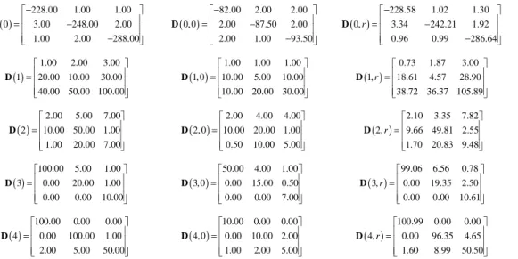
We consider a 3-state BMAP with M =4 distinct batch sizes as specified in the first column

of Table 1. Based on this parameter set, a trace file with n=200,000 arrivals and

corresponding batch sizes is generated. This trace file is used as input for the EM algorithm in order to derive estimates of the (known) parameter set of the BMAP. The parameter set shown in the second column of Table 1 serves as initial parameter set for the estimation

procedure. Running the EM algorithm for r=400 iterations on this trace file results in the

estimated parameter set presented in the third column of Table 1. As mentioned above, Table 1 shows that zero entries in the initial parameter set are preserved in the corresponding elements of the successive estimates. We observe that most parameter estimates calculated by the EM algorithm are quite close to the corresponding values of the original parameter set. As shown in [4], BMAPs are over-parameterized, i.e., different parameter sets can yield the same distribution. As a consequence, both the original and the estimated parameter set can differ while still showing similar quality, i.e., likelihood, for the considered trace file. Thus, the quality of the estimated BMAP should be compared to the quality of the original parameter set by the ratio of their likelihoods. With a ratio of 1.000029, this comparison evidently shows that the original and estimated parameter set have quite the same quality, although they (slightly) differ in parameter values.

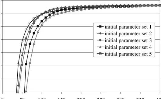
Additionally, the EM algorithm has been applied for 5 different (random) initial parameter sets for the considered trace file. Figure 4 plots the logarithm of the likelihood versus the number of iterations for these 5 estimation runs. While the likelihood differs significantly for small number of iterations, this difference diminishes rapidly for an increasing number of iterations, i.e., beyond 250 iterations all likelihood estimates are nearly the same. Thus, for a

given convergence criteria, where successive estimates differs only up to a predefined ε,

( ) 228.00 1.00 1.00 0 3.00 248.00 2.00 1.00 2.00 288.00 −     =_ − _ −     D ( ) 82.00 2.00 2.00 0,0 2.00 87.50 2.00 2.00 1.00 93.50 −     =_ − _ −     D ( ) 228.58 1.02 1.30 0, 3.34 242.21 1.92 0.96 0.99 286.64 r −     =_ − _ −     D ( ) 1.00 2.00 3.00 1 20.00 10.00 30.00 40.00 50.00 100.00     =_{ }     D ( ) 1.00 1.00 1.00 1, 0 10.00 5.00 10.00 10.00 20.00 30.00     =_{ }     D ( ) 0.73 1.87 3.00 1, 18.61 4.57 28.90 38.72 36.37 105.89 r     =_{ }     D ( ) 2.00 5.00 7.00 2 10.00 50.00 1.00 1.00 20.00 7.00     =_{ }     D ( ) 2.00 4.00 4.00 2, 0 10.00 20.00 1.00 0.50 10.00 5.00     =_{ }     D ( ) 2.10 3.35 7.82 2, 9.66 49.81 2.55 1.70 20.83 9.48 r     =_{ }     D ( ) 100.00 5.00 1.00 3 0.00 20.00 1.00 0.00 0.00 10.00     =_{ }     D ( ) 50.00 4.00 1.00 3,0 0.00 15.00 0.50 0.00 0.00 7.00     =_{ }     D ( ) 99.06 6.56 0.78 3, 0.00 19.35 2.50 0.00 0.00 10.61 r     =_{ }     D ( ) 100.00 0.00 0.00 4 0.00 100.00 1.00 2.00 5.00 50.00     =_{ }     D ( ) 10.00 0.00 0.00 4,0 0.00 10.00 2.00 1.00 2.00 5.00     =_{ }     D ( ) 100.99 0.00 0.00 4, 0.00 96.35 4.65 1.60 8.99 50.50 r     =_{ }     D

654000 654050 654100 654150 654200 654250 654300 654350 0 50 100 150 200 250 300 350 400 number of iterations log (lik elih ood

) initial parameter set 1

initial parameter set 2 initial parameter set 3 initial parameter set 4 initial parameter set 5

Figure 4. Convergence behavior for different (random) initial parameter sets

different initial parameter sets result in estimated parameter sets of similar quality with a slightly different number of iterations required for their estimation. Figures 5 and 6 show the maximum relative percentage change and absolute change in parameter values of two successive iterations. Regardless of the parameter values of the initial parameter set, the maximum relative percentage change is below 10% after 50 iterations and below 2% after 400 iterations. Similarly, as depicted in Figure 6, the absolute change in parameter values is below 0.1 after 100 iterations and below 0.01 after 400 iterations for almost all initial parameter sets. In summary, random initialization has proven to be an easy and sufficient way for determining initial parameter sets.

1e-01 1e+00 1e+01 1e+02 0 50 100 150 200 250 300 350 400 number of iterations rel at iv e p ercen tage ch an ge [ %

] initial parameter set 1

initial parameter set 2 initial parameter set 3 initial parameter set 4 initial parameter set 5

Figure 5. Maximum relative percentage change in parameter values

1e-03 1e-02 1e-01 1e+00 1e+01 0 50 100 150 200 250 300 350 400 number of iterations abs o lut e change

initial parameter set 1 initial parameter set 2 initial parameter set 3 initial parameter set 4 initial parameter set 5

Figure 6. Maximum absolute change in parameter values

4 Traffic Modeling of IP Networks utilizing the BMAP

4.1 BMAP Traffic Modeling Framework

As stated above, we customize the batch Markovian arrival process such that different lengths

of IP packets are represented by rewards (i.e., batch sizes of arrivals) of the BMAP. In order to represent an aggregated traffic stream utilizing the BMAP, we apply the parameter estimation procedure introduced in Section 3 for a BMAP with N transient states and M

distinct batch sizes. The choice of N and M is crucial for an accurate capturing of the

interarrival process and the reward process of the aggregated traffic, respectively. As shown above, the computational complexity of the EM algorithm is independent of the choice of M. Thus, this modeling approach can be effectively applied for arbitrary packet length (i.e., reward) distributions by an increasing value of M.

The underlying trace file, which constitutes the aggregated traffic, comprises packet interarrival-times as well as the corresponding packet lengths. Recalling the BMAP definition of Section 2, the mapping process of packet lengths to BMAP rewards results in a BMAP

parameter set, i.e., π and D

( )

0 ,…,D

( )

M , of reasonable size

(

M +1

)

N2+N. We map the

packet lengths onto the discrete packet lengths s , for 1 m ≤ m ≤ M, where s is the average m

packet length of all packets of the considered trace comprising packet lengths between

(

1

)

L⋅ m− M bytes and L m M⋅ bytes, where L denotes the maximum packet length of the

considered IP network. In the case of Ethernet local area networks (LAN) the maximum transfer unit (MTU) of 1500 bytes determines this maximum packet length. Therefore,

arrivals with batch size m, 1 ≤ m ≤ M, represent packet arrivals with a packet length of s m

bytes. Note, that this mapping process is applied for ease of notation only. Without this mapping, the proposed estimation procedure can be applied for estimating the rate matrices

( ) ( )

0 , s1 , ,

( )

sM

D D … D , where rate matrices D

( )

m , m∉

{

0, ,s1 …,sM

}

, are empty. The

estimation of these matrices obviously requires the same computational effort. Moreover, the

estimated matrices are identical to the matrices D

( )

0 ,…,D

( )

M , which are computed when

the mapping process is applied. In [11], we presented an aggregated traffic model for the Universal Mobile Telecommunication Systems (UMTS) based on measured trace data, which successfully employs this traffic modeling framework.

4.2 IP Traffic Measurement and Modeling

In order to illustrate the effectiveness and accuracy of the proposed traffic model for measured IP traffic, we conducted detailed traffic measurements at the Internet service provider (ISP) dial-up modem/ISDN link of the University of Dortmund. Note that we have also applied the BMAP traffic modeling approach to various other IP traffic traces (LAN and WAN) and observe similar results in terms of effectiveness and accuracy compared to the trace considered in this paper. Thus, it is fair to say that the proposed modeling approach

comprises general applicability in networking environments. These measurements were

performed by the software package TCPdump running on a Linux host that sniffs all IP

packets in the Ethernet segment between the MaxTNT dial-up routers and the Internet router. For all IP datagrams sourced or targeted by dial-up modems the TCP/IP header information in conjunction with a timestamp of the arrival-time have been recorded and stored for offline processing. Note that the TCP/IP header information includes the packet length [18].

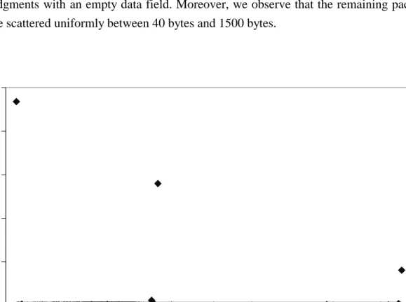
Similarly to observations in other LANs and wide area networks [19], [20], the analysis of the packet length distributions revealed that the packet lengths of all relevant TCP applications follow to a large extent a discrete distribution, i.e., packet lengths of 40 bytes, 576 bytes, and 1500 bytes dominate with an overall percentage of 80% of all TCP packets (see Figure 7). This observation can be explained because they correspond to the maximum transfer units of the used network protocols. Most application protocols like FTP, HTTP, POP3, and SMTP are used to transfer relatively large data blocks (as opposed to many small packets in real-time applications). Therefore, in order to reduce overhead, as many packets as possible are filled up to the MTU of the underlying protocol, which typically are 1500 bytes in the Ethernet protocol and 576 bytes in the serial line Internet protocol (SLIP). The choice between a MTU of 576 bytes or 1500 bytes depends on the network configuration of the dial-up client. The large amount of 40 bytes packets is to a large extent caused by TCP acknowledgments with an empty data field. Moreover, we observe that the remaining packet lengths are scattered uniformly between 40 bytes and 1500 bytes.

0.0 0.1 0.2 0.3 0.4 0.5 0 200 400 600 800 1000 1200 1400

packet length in bytes

probability mass function

The aggregated traffic model utilizes these observations where different reward values of the BMAP represent different discrete packet lengths. Thus, the parameter estimation

procedure is applied for a BMAP with M =3 distinct batch sizes using a trace file of

1,500,000 samples (measured 10.00 a.m. 13 December 2000 at the dial-up modem/ISDN link) comprising interarrival-times and the corresponding packet lengths. By empirical

observations, we found that a 3-state BMAP

(

N =3

)

is sufficient in order to capture the

interarrival process of the considered trace. Recall that the choice of M is crucial for the

mapping process of packet lengths to BMAP rewards and corresponds to, but is not restricted by the fact that a large amount of packets comprise three different packet lengths (see Figure

7). As defined above, the average packet lengths s (m M =3) of our measurements are as

follows: s1=94 bytes, s2 =575 bytes, and s3 =1469 bytes.

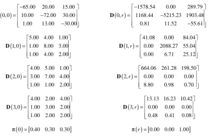
Table 2 presents the initial parameter set π

( )

0 and D

( )

0, 0 ,…,D

( )

3, 0 as well as the

estimated parameter set π

( )

r and D

( )

0,r ,…,D

( )

3,r after r=51 iterations of the EM

algorithm introduced in Section 3. Convergence is reached when each component of φ

( )

r

and φ

(

r+1

)

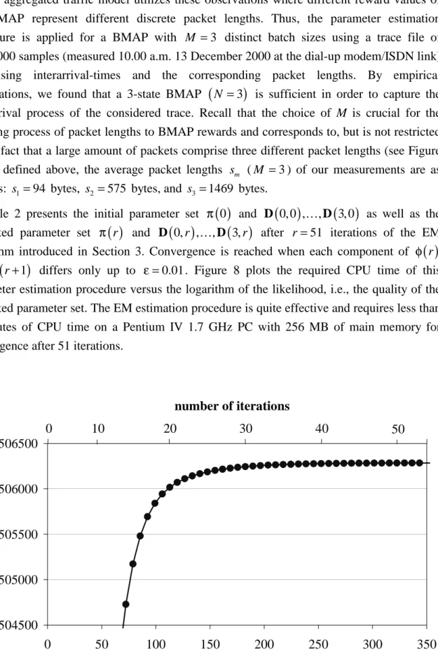
differs only up to ε =0.01. Figure 8 plots the required CPU time of this

parameter estimation procedure versus the logarithm of the likelihood, i.e., the quality of the estimated parameter set. The EM estimation procedure is quite effective and requires less than 6 minutes of CPU time on a Pentium IV 1.7 GHz PC with 256 MB of main memory for convergence after 51 iterations.

504500 505000 505500 506000 506500 0 50 100 150 200 250 300 350

CPU time in sec.

log (likelihood)

0

number of iterations

10 20 30 40 50

4.3 Comparative Study of Aggregated IP Traffic Modeling

The following shows the effectiveness of our BMAP modeling approach, compared with a

3-state MMPP

(

N =3

)

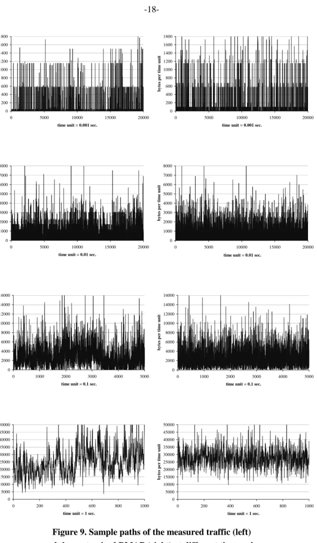
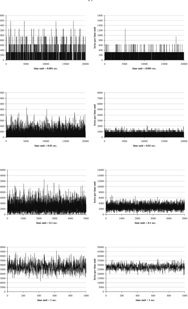
and Poisson process, by means of visual inspection of sample paths

over multiple time scales, by presenting important statistical properties, by formal analysis of traffic burstiness as well as by investigations of queuing behavior. Figure 9 and 10 plot sample paths of the measured traffic (Figure 9, left) compared with the sample paths of the aggregated traffic streams of the customized BMAP using the estimated parameter set of Table 2 (Figure 9, right), the MMPP (Figure 10, left), and the Poisson process (Figure 10, right), respectively. For sample path construction of the MMPP and the Poisson process, we associate the average packet length of all IP packets comprising 315 bytes with the arrival-times of the MMPP and the Poisson process. The aggregated traffic streams of the MMPP and the Poisson utilized for sample-path construction comprise the same number of samples as the

measured trace file. Note, that the parameter matrices D

( )

0 and D

( )

1 of the MMPP have

also been estimated by means of the EM algorithm for BMAP. This is accomplished by

restriction of D

( )

1 to diagonal entries that are associated with the state-dependent Poisson

arrival-rates of the MMPP. The arrival-rate of the Poisson process is naturally given by the mean arrival-rate of the measured trace file. In order to show the effectiveness of our approach these sample paths are plotted on four different time scales, i.e. 0.001 sec, 0.01 sec, 0.1 sec, and 1.0 sec. Figure 9 and 10 evidently show that the customized BMAP authentically captures the average transferred data volume per time unit and exhibits traffic burstiness over multiple time scales in the considered scenario. Moreover, these sample paths show the clear advantage of the customized BMAP over the MMPP and the Poisson process, which fail to capture the original sample path over almost all time scales.

In order to emphasize these observations, we investigate the distribution of the transferred data volume per time unit for the measured trace, customized BMAP, the MMPP, and the

( ) 65.00 20.00 15.00 0, 0 10.00 72.00 30.00 1.00 13.00 30.00 −     =_ − _ −     D ( ) 1578.54 0.00 289.79 0, 1168.44 5215.23 1903.48 0.81 11.52 55.61 r −     =_ − _ −     D ( ) 5.00 4.00 1.00 1, 0 1.00 8.00 3.00 1.00 4.00 2.00     =_{ }     D ( ) 41.08 0.00 84.04 1, 0.00 2088.27 55.04 0.00 6.71 25.12 r     =_{ }     D ( ) 4.00 5.00 1.00 2, 0 3.00 7.00 4.00 1.00 1.00 2.00     =_{ }     D ( ) 664.06 261.28 198.50 2, 0.00 0.00 0.00 8.80 0.98 0.70 r     =_{ }     D ( ) 4.00 2.00 4.00 3, 0 1.00 3.00 2.00 1.00 2.00 2.00     =_{ }     D ( ) 13.13 16.23 10.42 3, 0.00 0.00 0.00 0.48 0.41 0.08 r     =_{ }     D ( )0 =[0.40 0.30 0.30] π π( )r =[0.00 0.00 1.00]

0 200 400 600 800 1000 1200 1400 1600 1800 0 5000 10000 15000 20000

time unit = 0.001 sec.

byte s pe r ti m e uni t 0 200 400 600 800 1000 1200 1400 1600 1800 0 5000 10000 15000 20000

time unit = 0.001 sec.

byte s pe r ti m e uni t 0 1000 2000 3000 4000 5000 6000 7000 8000 0 5000 10000 15000 20000

time unit = 0.01 sec.

byte s pe r ti m e uni t 0 1000 2000 3000 4000 5000 6000 7000 8000 0 5000 10000 15000 20000

time unit = 0.01 sec.

byte s pe r ti m e uni t 0 2000 4000 6000 8000 10000 12000 14000 16000 0 1000 2000 3000 4000 5000

time unit = 0.1 sec.

byte s pe r ti m e uni t 0 2000 4000 6000 8000 10000 12000 14000 16000 0 1000 2000 3000 4000 5000

time unit = 0.1 sec.

byte s pe r ti m e uni t 0 5000 10000 15000 20000 25000 30000 35000 40000 45000 50000 0 200 400 600 800 1000

time unit = 1 sec.

byte s pe r ti m e uni t 0 5000 10000 15000 20000 25000 30000 35000 40000 45000 50000 0 200 400 600 800 1000

time unit = 1 sec.

byte s pe r ti m e uni t

Figure 9. Sample paths of the measured traffic (left) and the customized BMAP (right) at different time scales

0 200 400 600 800 1000 1200 1400 1600 1800 0 5000 10000 15000 20000

time unit = 0.001 sec.

byte s pe r ti m e uni t 0 200 400 600 800 1000 1200 1400 1600 1800 0 5000 10000 15000 20000

time unit = 0.001 sec.

byte s pe r ti m e uni t 0 1000 2000 3000 4000 5000 6000 7000 8000 0 5000 10000 15000 20000

time unit = 0.01 sec.

byte s pe r ti m e uni t 0 1000 2000 3000 4000 5000 6000 7000 8000 0 5000 10000 15000 20000

time unit = 0.01 sec.

byte s pe r ti m e uni t 0 2000 4000 6000 8000 10000 12000 14000 16000 0 1000 2000 3000 4000 5000

time unit = 0.1 sec.

byte s pe r ti m e uni t 0 2000 4000 6000 8000 10000 12000 14000 16000 0 1000 2000 3000 4000 5000

time unit = 0.1 sec.

byte s pe r ti m e uni t 0 5000 10000 15000 20000 25000 30000 35000 40000 45000 50000 0 200 400 600 800 1000

time unit = 1 sec.

byte s pe r ti m e uni t 0 5000 10000 15000 20000 25000 30000 35000 40000 45000 50000 0 200 400 600 800 1000

time unit = 1 sec.

byte s pe r ti m e uni t

Figure 10. Sample paths of the MMPP (left) and the Poisson process (right) at different time scales

0.94 0.95 0.96 0.97 0.98 0.99 1.00 0 250 500 750 1000 1250 1500 1750 2000 bytes per time unit (0.001 sec.)

cu m u la ti ve di st ri buti on func ti on measured traffic customized BMAP MMPP Poisson process 0.6 0.7 0.8 0.9 1.0 0 500 1000 1500 2000 2500 3000 3500 4000 bytes per time unit (0.01 sec.)

cu m u la ti ve di st ri buti o n func ti on measured traffic customized BMAP MMPP Poisson process 0.0 0.1 0.2 0.3 0.4 0.5 0.6 0.7 0.8 0.9 1.0 0 2000 4000 6000 8000 10000

bytes per time unit (0.1 sec.)

cu m u la ti ve di st ri buti o n func ti on measured traffic customized BMAP MMPP Poisson process 0.0 0.1 0.2 0.3 0.4 0.5 0.6 0.7 0.8 0.9 1.0 0 10000 20000 30000 40000 50000 60000 bytes per time unit (1 sec.)

cu m u la ti ve di st ri buti o n func ti on measured traffic customized BMAP MMPP Poisson process

Figure 11. Cdfs of data rates on different time scales

Poisson process, respectively. Figure 11 plots the cumulative distribution function (cdf) of transferred data volume for the time scales 0.001 sec, 0.01 sec, 0.1 sec, and 1 sec. We observe, that the cdf of the measured traffic and the customized BMAP performs different on the considered time scales. For the time scales 0.01 sec and 0.1 sec the cdf of the measured trace is accurately represented by the customized BMAPs cdf. On the smallest time scale, i.e., 0.001 sec, both cdfs exhibit the same trends whereas the cdf of the measured trace is not

exactly matched by the customized BMAP. This can be explained by the choice of M =3 for

the customized BMAP, where the lack of various different packet lengths leads to the discrete

steps in shape of the BMAPs cdf. By increasing the value of M, the differences of the cdfs on

this time scale diminish. On the other hand, the shape behavior of the cdfs on the largest time scale shows significantly differences, whereas the trends in both cdfs are roughly identically.

Here, the BMAPs second essential parameter, i.e., the number of transient states N, does make

the trick. By increasing the number of transient states (N =3 in this study), the shape of the

BMAPs cdf will be similar to the cdf of the measured trace. This is, because the flexibility for

transitions between states is rapidly increased by the choice of N (see Section 3), i.e., an

increased number of transient states is actually capable to generate very low data rates (head of the cdf) and very high data rates (tail of the cdf) even on large time scales. As expected, the cdf of the Poisson process performs badly and shows significant differences to the cdf of the measured traffic over all considered time scales. Obviously, the MMPP outperforms the Poisson process, but is inferior in capturing the cdf of the measured traffic, compared with the customized BMAP over all considered time scales.

time unit in sec. mean standard deviation skewness kurtosis measured traffic 27.63 153.02 6.72 52.77 customized BMAP 27.70 157.90 8.12 84.34 MMPP 27.65 118.39 5.58 42.73 Poisson process 27.65 93.37 3.38 14.46 measured traffic 276.27 697.46 4.21 29.03 customized BMAP 277.01 662.32 3.82 23.14 MMPP 276.47 491.13 2.81 13.84 Poisson process 276.49 295.82 1.07 4.14 measured traffic 2762.64 2240.81 1.44 6.15 customized BMAP 2770.10 2191.71 1.27 5.15 MMPP 2764.61 1672.45 0.90 4.21 Poisson process 2764.86 933.00 0.33 3.11 measured traffic 27621.50 10954.80 0.60 3.21 customized BMAP 27697.30 6929.95 0.41 3.19 MMPP 27643.70 5413.94 0.28 3.05 Poisson process 27643.70 2972.29 0.03 2.94 0.001 0.01 0.1 1

Table 3. Statistical properties of data rates on different time scales

Table 3 presents additionally statistical properties for the data rates of the measured traffic, the BMAP, the MMPP, and the Poisson process, on different time scales in terms of mean, standard deviation, skewness, and kurtosis. Recall, that the mean gives the center of the distribution and the standard deviation measures the dispersion about the mean. The third moment about the mean measures skewness, the lack of symmetry, while the forth moment measures kurtosis, the degree to which the distribution is peaked. In Table 3, skewness and kurtosis are standardized by an appropriate power of the standard deviation. We observe, that mean and standard deviation of the measured traffic and the customized BMAP perform quite similar over the considered time scales, with exception of the BMAPs standard deviation on the largest time scale. The skewness of the measured traffic is quite similar on medium time scales, i.e., 0.01 sec and 0.1 sec, while the customized BMAP overestimates the skewness on the smallest time scale and underestimates it on the largest time scale. Furthermore, the last column of Table 3 indicates, that kurtosis, i.e., peakedness, is well captured on the three largest time scales, whereas the BMAP significantly exceeds the measured traffic on the smallest time scale. This is, because on the smallest time scale the various packet lengths of

the measured traffic cannot be represented exactly by only three (M =3) different reward

values, i.e., packet lengths. This effect diminishes with increasing value of M. Moreover,

Table 3 evidently shows, that the MMPP as well as the Poisson process are clearly inferior compared with the customized BMAP and badly capture standard deviation, skewness and kurtosis, over all considered time scales.

These observations are emphasized by the analysis of traffic burstiness, which can be

expressed in terms of the Hurst parameter H. Figure 12 plots the R/S statistics [21] of the

0.0 0.5 1.0 1.5 2.0 2.5 3.0 1.0 1.5 2.0 2.5 3.0 3.5 4.0 log(k) log(R/S) measured traffic H = 0.6785 customized BMAP H = 0.6418 MMPP H = 0.6408 Poisson process H = 0.5558

Figure 12. R/S statistic plot of the measured traffic and the analytically tractable models

degree of traffic burstiness H, can easily derived for a considered time scale by the slopes of

linear regression plots of the R/S statistics. As expected, the Poisson process (H = 0.5558)

fails to capture the traffic burstiness, while the MMPP (H = 0.6408) and the customized

BMAP (H = 0.6418) both indicate a significant amount of traffic burstiness compared to the

Hurst parameter of the measured traffic (H = 0.6785).

The practical applicability of our BMAP modeling approach can be emphasized by the analysis of the queuing performance. As proposed in [1], we utilize a simple queuing model with deterministic service time and unlimited capacity for investigations of the complement distribution of the queue length. Figure 13 depicts the complement distribution of the queue length Q of the BMAP/D/1 queuing system, the MMPP/D/1 queuing system and the M/D/1 queuing system (using the Poisson process), compared with the simulations performed with

the measured traffic for different traffic intensities ρ. It is obvious that the BMAP model

shows a similar behavior in terms of queuing performance for low traffic intensities, i.e.,

0.3

ρ = and ρ =0.4. For traffic intensities of ρ =0.5 and ρ =0.6 the customized BMAP

matches the distribution of the measured traffic up to medium queue length. As expected, the Poisson process performs badly for all considered traffic intensities. Again, the MMPP outperforms the Poisson process, but is significantly inferior in capturing the complement distribution of the queuing length, compared with the customized BMAP for all considered traffic intensities.

1e-04 1e-03 1e-02 1e-01 1e+00

1e+01 1e+02 1e+03 1e+04

x P{ Q ≥ x} measured traffic customized BMAP MMPP Poisson process ρ = 0.3 1e-04 1e-03 1e-02 1e-01 1e+00

1e+01 1e+02 1e+03 1e+04

x P{ Q≥ x} measured traffic customized BMAP MMPP Poisson process ρ = 0.4 1e-04 1e-03 1e-02 1e-01 1e+00

1e+01 1e+02 1e+03 1e+04 1e+05

x P{ Q ≥ x} measured traffic customized BMAP MMPP Poisson proces ρ = 0.5 1e-04 1e-03 1e-02 1e-01 1e+00

1e+01 1e+02 1e+03 1e+04 1e+05

x P{ Q ≥ x} measured traffic customized BMAP MMPP Poisson process ρ = 0.6

Figure 13. Complement distribution of queue length Q of single server queue with deterministic service time for different traffic intensities ρ

5 Conclusions

We introduced an efficient and numerical stable method for estimating the parameters of a batch Markovian arrival process (BMAP) with the EM algorithm. The contribution of the paper is two-fold. First, we show how the randomization technique and a stable calculation of Poisson jump probabilities can effectively be utilized for the computation of the time-dependent conditional expectation of a continuous-time Markov chain (CTMC) required by the estimation step (E-step) of the EM algorithm. Second, based on these methodological results, we introduce a framework for traffic modeling of aggregated IP traffic utilizing the BMAP, which both is analytically tractable and closely captures the statistics of the measured traffic data. The key idea of this aggregated traffic model lies in customizing the batch Markovian arrival process such that different lengths of IP packets are represented by reward values, i.e., batch sizes of arrivals, of the BMAP. In order to demonstrate the advantages of the BMAP modeling approach over other widely used analytically tractable models, we compare the customized BMAP with the MMPP and the Poisson process by means of visual inspection of sample paths over four different time scales, by presenting important statistical properties and by formal analysis of traffic burstiness using R/S statistics. Furthermore, investigations of queuing behavior demonstrate the practical applicability of aggregated traffic modeling using the BMAP.