Discrete-Time Scheduling under Real-Time Constraints

Discrete-Time Scheduling under Real-Time Constraints

Eduard Cerny1

, Yuke Wang2

, Mostapha Aboulhamid1 1

Laboratoire LASSO, Dép. d’IRO, Université de Montréal

2

Dept. ECE, Concordia University Montréal (Québec) Canada

Abstract

We introduce a new method for scheduling under real-time constraints that is suitable for synchronous system implementations. The input specification is in the form of timing diagrams in which the occurrence times of signal transitions or actions are related by linear constraints, expressing the assumptions on the input actions (the environment) and the commitments on the output actions. Provided that the specification is causal, we give an algorithm for deriving ASAP and ALAP relative schedules for the output actions. We then present a new algorithm for determining whether a given clock period is correct. Based on a schedule and a valid clock period, we transform the specification into a discrete-time relative schedule. Such a schedule serves as the basis for implementing a synchronous state-machine controller.

Keywords: Timing diagrams, relative scheduling, real-time constraints, synchronous state machines. 1 Introduction

High-level synthesis of digital hardware for real-time applications [10, 22], as well as the synthesis of interface transducers and controllers [2, 4, 11, 12], require to perform scheduling of actions and operations under explicit real-time constraints. In [22], operations with unknown duration were modeled using unbounded delays from the start of such an operation to the start of any successor operation that depended on it. Linear timing constraints were used to restrict the occurrence times of operations relative to each other. Since linear constraints may impose restrictions on the time separation of the anchor operations, thus making the specification unrealizable for all possible durations of the anchor operation, the authors of [22] defined the so-called well-posedness condition of the timing constraints of the specification. In interface transducer synthesis, the situation is to some extent similar, in that events are constrained by timing onstraints (linear, latest, and earliest) [4, 7]. Here, events usually represent signal transitions or enabling situations for data to appear on busses. The synthesis has, however, much in common with the problem of scheduling under real-time constraints used in high-level synthesis.

In this paper, we describe a relative scheduling method for specifications inspired by timing diagrams as formalized in [14, 15, 19, 21]. In summary, the main distinguishing charactersitics of our approach are as follows:

- Instead of dealing with operations (that have duration) and signal transitions (events), we consider only instantaneous actions. These then can be used in pairs to delimit the start and the end of an operation, or to model individually some specific events or signal transitions in the system. This approach has been quite effective in modeling systems using (real-time) process algebras.

- We explicitly distinguish output (or internal) actions whose occurrence time is under the control of the synthesized device, and input actions whose occurrence time is controlled by the environment. In both cases, the occurrence time of an action may be restricted by the occurrence time of some preceding actions (input or output). We allow linear, latest and earliest type of timing constraints, however, in this paper we consider only linear constraints, since these are the source of noncausality in TD specifications and require special techniques for deriving schedules.

- To provide means for describing timing assumptions that can be made on the occurrence time of input actions, and the limits on the reaction time of the output actions, we distinguish two kinds of timing constraints, assume and commit, respectively. This allows to state what assumptions are made on the environment and then take this information into account during synthesis (assumption-based reasoning); this is more realistic than assuming that any duration of, say, an input operation is possible [22].

- Allowing finite assumption constraints requires a generalization of the well-possedness condition of the system of constraints. We have recognized this in the context of interface specifications and their compatibility verification [15] as a problem of causality. Causality conditions allow us to use a more complex structure of a specification than in [22] such that the input and output actions can be intermixed as in timing diagrams.

The contributions of the present paper are:

- A method is presented for deriving a relative schedule for output and internal actions, relative to the so-called trigger actions [15]. We can guarantee the existence of the schedule only if the specification is causal.

- The timing constraints can be given in dense time (the reals), however, hardware implementation is often carried out using synchronous design techniques where all operations are synchronized to a common clock of period C. We present a method for verifying that a period C is valid, and then produce a discrete-time relative schedule for the output actions in which the time unit is the clock tick. Such a schedule can be used in existing synthesis methods, e.g., [10, 22].

This methodology is centered around the so called Hierarchical Annotated Action Diagrams (HAAD) [17, 18]. Leaf diagrams correspond to the timing diagrams used as the basis for synthesis in this paper. The hierarchical diagrams form more complex behaviors using composition operators over leaf and other hierarchical diagrams. The operators are inspired by process algebras (parallel with causal rendez-vous communication, concatenation, loop, delayed choice, and exception handling). All diagrams can also be annotated by VHDL procedures, variables, and predicates. For a useful subset of this specification language we have defined the formal semantics and provided axiomatization [19], including conversion to a normal form that can be used to transform the specification to a network of Timed Automata for verification using existing tools. Furthermore, the verification of causality and compatibility on leaf-level diagrams can be efficiently carried out using Constraint Logic Programming based on Relational Interval Arithmetic [20, 21].

The paper is organized as follows: Section 2 introduces basic concepts about timing diagrams, causality, and scheduling. Section 3 describes the determination of a valid clock period and the derivation of a discrete-time relative schedule; it also contains a complete example. Section 4 concludes the presentation.

2 Background Information

2.1 Timing diagrams and the causality property

In this section, we introduce some background concepts about timing diagrams, event graphs of timing diagrams, and the causality property [15, 17].

Definition 1: There is a global time variable T that increases monotonically. The current time is the value of the variable T. Initially, the global time variable is reset to some real value τ. Let E = {e₁, e₁, …, e_n}be a set of events. A time-stamp variable

t

_i is associated with each event e_i; t_i = x means that e_i occurs when the value of the time variable T becomes x. Current time and time stamps take on finite, possibly unbounded, real values.

Definition 2: Let E = {e₁, e₁, …, e_n} be a set of events. c_ij = (e_i, e_j, [l_ij, u_ij]) represents the constraint l_ij≤ t_j -t_i≤ u_ij on the separation between the occurrence times of e_i, e_j∈ E. We call e_i the source and e_j the sink of the constraint. A constraint c_ij = (e_i, e_j, [l_ij, u_ij]) is a precedence constraint if u_ij≥ l_ij > 0, and a concurrency constraint if u_ij≥ 0 ≥ l_ij.

Let E_in⊆ E the set of all input events, and E_out⊆ E the set of all output events, E_in∩ E_out = ∅, E = E_in∪ E_out

Definition 3: A timing diagram TD = (E, C) is determined by its set of events E and the set CS of constraints over E. A constraint c_ij = (e_i, e_j, [l_ij, u_ij]) ∈ C such that e_i and e_j are of different directions must be a precedence constraint.

The constraints in CS have one of two possible intents. It is an assume constraint if the sink is an input event; otherwise it is a commit constraint. Assume constraints delimit the expected or assumed behavior of the environment, while the commit constraints define the limits on the occurrence times of the output events. In other words, the device implementation must satisfy the commit constraints, provided that the environment satisfies the assumptions.

Definition 4: Consider a timing diagram TD = (E, C) with c_ij = (e_i, e_j, [l_ij, u_ij]). The event graph EG=(V,E_g) of TD is a directed weighted graph where the vertex set V is E, and for each constraint c=(ei,ej,[lij,uij])∈C in TD, there are two edges in E_g, (e_i, e_j) labeled by u_ij, and (e_j, e_i) labeled by -l_ij; the label is called the weight of the edge.

An edge (e_i, e_j) in EG labeled by weight

w

_ij represents the constraint t_j −t_i ≤w_ij. That is, a two-sided constraint in TD is represented by two one-sided constraints in EG.

Example 1: Figure 1(a) shows a TD where E_out = { e₁, e₃}, E_in = { e₂, e₄}. The constraints (e₁, e₂, [l₁₂, u₁₂]) and (e₁, e₃, [l13, u13]) are assume constraints, the other two are commit constraints. Its corresponding EG is given by Figure 1(b).

A ssu m e C o m m it [l1 2, u1 2] [l_{2 4}, u_{2 4}] u3 4 [l1 3, u1 3] e1 o u t e2 in e3 in e4 o u t -l1 2 u1 2 -l2 4 u2 4 -l1 3 u1 3 -l3 4 e2 e1 e3 e4 (a ) _{(b )}

A path p(e_i, e_j) in EG from e_i to e_j is a sequence of edges (e_i, e_j1)(e_j1, e_j2) … (e_jk-1, e_jk)(e_jk, e_j). A cycle is a path p(e_i, e_i). The weight of a path is the sum of the weights of all edges along the path. The shortest path from

e

_i to

e

_j is the path whose weight is the smallest from among all the paths from e_i to e_j. The constraint system CS is consistent if there is no cycle with negative weight in EG, otherwise CS is inconsistent [3].

An event graph can be checked alone for consistency which is a minimal form of realizability [3, 14, 15]. It assures that the constraint system CS has a solution and thus an occurrence time can be assigned to every event. As pointed out in [14, 15, 17], the notion of consistency of the event graph of a TD is insufficient for constructing correct implementations. In fact, inconsistency is a special case of non-causality. We now introduce causal TDs [15, 17]:

Definition 5: In an EG, the maximum separation time from event e_j to event e_i is defined as max (t_i - t_j), where t_i and t_j satisfy the TD constraints [9]. If max (t_i - t_j) < 0, then event e_i strictly precedes event e_j. It is well known that the maximum separation from ej to eiis the shortest distance from ej to eiin EG [3].

We describe next the execution semantics of the model underlying a TD specification. They are based on the notion of a block of events.

Definition 6: Consider the event graph EG of a timing diagram TD = (S, E, C). Let {EB_i} be a partition over the event set E = ∪EB_i, EB_i∩ EB_j = ∅, ∀i, EB_i ⊆ E_in or EB_i ⊆ E_out. Each EB_i is called an event block.

Let E_ij = {e_k∈ EB_j | ∃ e_l∈ EB_i such that there is an edge from e_k to e_l or from e_l to e_k}, i.e., E_ij contains all events from EB_j related by a constraint to some event in EB_i. The block EB_j is the predecessor of the block EB_i, denoted by EB_j = pred(EB_i), if events e_j∈ E_ij strictly precede all events e_i∈ EB_i, i.e., max (t_j -t_i) < 0. In this case, the events in E_ij are called the triggers of EB_i in EB_j. The local constraints of EB_i are those constraints of CS that (1) relate pairs of events in EB_i or (2) relate events in EB_i to its triggers. The partition { EB_i }must also satisfy the following property:

Property 1: For all pairs of blocks EB_i, EB_j∈ { EB_i }, if E_ij≠∅, then either EB_i = pred(EB_j) or EB_j = pred(EB_i). In a consistent CS, the relation pred induces a partial order (<) over blocks.

An event block EBi is enabled when all its trigger events have occurred. EBi becomes enabled at time t if the last

trigger(s) occurred at t. An enabled event block EB_i is fixed when the occurrence times of all its events are assigned a value such that the local constraints of the block are satisfied, given the occurrence times of the triggers. If no such assignment exists then the block cannot be fixed.

Definition 7: A partition { EB_i }of EG is causal iff it satisfies Property 1 and every event block can be enabled and fixed. A TD is causal if its EG has a causal partition.

Theorem 1 ([15, 17]): A TD is causal iff for each pair of triggers of each block the maximum separation between the triggers as computed using the local constraints of the block is strictly greater than the maximum separation of that pair computed over the entire EG.

In the rest of this paper, we assume that all TDs are causal with a partition { EB_i }. 2.2 Scheduling of events under TD constraints

In the preceding section, we introduced two kinds of constraints in TDs: assume and commit. We can schedule only the output events controlled by the commit constraints, since the input events related by the assume constraints are controlled by the environment. In this section, we present scheduling algorithms for output events of a causal TD. Some of the concepts introduced here are similar as in [10, 22].

Definition 8: A schedule of a TD is a function that assigns an occurrence time to each output event such that all commit constraints in the timing diagram are satisfied, given any occurrence times of the input events satisfying the assume constraints and the occurrence times of preceding output events. Such an assignment of occurrence times is called a valid assignment.

We first describe a method to fix an output block, assuming that all its triggers have occurred. The complete schedule for a causal TD can then be obtained block by block, following any total order derived from the partial order between blocks (Section 2.1).

Consider a block EB = {e_i} with its trigger set Tr = {Tr_j}, and let the occurrence time of trigger Tr_j be T_j. The occurrence times t_iof events e_i∈ EB is a function of T_j given by the local constraints of EB: −w_ki ≤t_k −t_i ≤ w_ik and

ji j i

ij t T w

w ≤ − ≤

− Let σ_jk be the shortest distance from Tr_j to e_k, and σ_kj the shortest distance from e_k to Tr_j. Lemma 1:

(1) For any event e1∈ EB and a trigger Trj of EB the following relations hold: -w1j ≤σj1≤ wj1 and -wj1 ≤σ1j≤ w1j,

where

w

_{j 1} and

w

_{1 j} are the weights between e₁ and Tr_j .

(2) For any two events e₁ and e₂ in EB, and an edge from e₁ to e₂ with weight w₁₂, the relations σ_j2≤ w₁₂+σ_j1 and σ_2j≤ w₂₁+σ_1j hold.

Proof:

(1) This follows directly from the definition of the shortest path σ_j1 ≤ w_j1 since w_j1 is a path weight, and in a consistent constraint graph we must have σj1 + w1j≥ 0 (no negative cycle), similarly for σ1j.

(2) Suppose that σ_j1 + w₁₂ < σ_j2. Therefore, the shortest distance from Tr_j to e₂ is not σ_j2 because the path underlying σj1 and the edge from e1 to e2 form a shorter path - contradiction. Q.E.D.

Lemma 2: In a causal TD, for all events e_i∈ EB, its triggers and the local constraints of EB, the following holds: } min{ } { max j ji Tr Tr ij j Tr Tr T T j j σ σ ≤ + − ∈

∈ , where Tj is the occurrence time of trigger Trj.

Proof: Let Tr₁ and Tr₂ be any two triggers of EB and e_i∈ EB. σ_1i + σ_i2 is the distance of the shortest path from Tr₁ to Tr₂ using local constraints of EB and passing through e_i. Since the system is causal, by Theorem 1, we have T₂ - T₁ < σ1i + σi2, which induces the condition T2 - σi2 < σ1i + T1. This holds for any pair Tr1, Tr2; therefore,

} min{ } { max j ji Tr Tr ij j Tr Tr T T j j σ σ ≤ + − ∈ ∈ . Q.E.D.

Proposition 1: For all events e_i ∈ EB and all triggers Tr_j∈Tr of EB, the following holds: } min{ } { max j ji Tr Tr i ij j Tr Tr T t T j j σ σ ≤ ≤ + − ∈ ∈ .

Proof: For any trigger Tr_j and event e_i, t_i - T_j≤σ_ji, i.e., ∀Tr_j∈ Tr, σ_ji + T_j≥ t_i, hence min{ _{j ji}}

Tr Tr i T t j σ + ≤ ∈ . We can

prove the other half of the inequality in a similar fashion. Q. E. D.

Corollary 1: For all ei∈ EB, min{ j ji} Tr Tr i T t j σ + =

∈ is a valid occurrence time assignment. So is max{Tr Tr j ij}

i T t j σ − = ∈ ,

i.e., either min or max is used for all e_i, but not mixed within one block, in general.

Proof: We need to prove that for any trigger Tr_j, and any pair of events e₁ and e₂, the following conditions are satisfied (1) t₂ - t₁≤ w₁₂, and (2) t₁ - T_j≤ w_j1 and T_j - t₁≤ w_1j.

We first prove (1). Since 1 min{ j j1}

Tr Tr T t j σ + = ∈

, there exist triggers Tr_a and TR_{b such that} } min{ ₁ 1 1 j j Tr Tr a a T T t j σ σ = + + = ∈ and _{2 2} min{ _{j j2}} Tr Tr b b T T t j σ σ = + + = ∈

. Based on the definition of t₁ and t₂, we have T_a + σ_a1≤ T_b + σ_b1

T_b + σ_b2≤ T_a + σ_a2, and then

t₂ - t₁≤ [T_a + σ_a2] - [T_a + σ_a1] = σ_a2 - σ_a1≤ w₁₂, and

t1 - t2≤ [Tb + σb1] - [Tb + σb2] = σb1 - σb2≤ w21, both by Lemma 1.

Hence, (1) is proven. Next we prove (2). Let Tr_j be an arbitrary trigger of EB. Since _{1 1} min{ _{j j1}}

Tr Tr a a T T t j σ σ = + + = ∈ , we have ∀Tr_j, Tj + σj1≥ t1. By Lemma 2, j j j j Tr Tr T T t j 1 1 1 ≥ max{ −σ }≥ −σ

∈ . Hence, Tj - σ1j≤ t1≤ Tj + σj1 ). It follows that

t₁ - T_j = [T_j + σ_j1 ] - T_j = σ_j1≤ w_j1, and T_j - t₁≤σ_1j≤ w_1j Q. E. D. Definition 9: Denote the shortest distance from e_k to Tr_j as - σS

(e_k, Tr_j) = σ_kj and be the shortest distance from Tr_j to e_kas σL

(e_k, Tr_j) = σ_jk. The time interval [max{ ( , )},min{ ( i, j)}] L j j j i S j j Tr e T Tr e

T +σ +σ is called the feasible interval of

i e, denoted by [ , ] i i e e L S . Moreover, i e S and i e

L are called the as-soon-as-possible (ASAP) and the as-late-as-possible (ALAP) types of relative schedules of the output events, respectively.

3 Discrete-Time Schedules

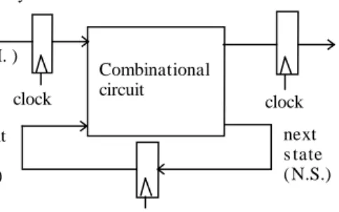
We discuss here the conversion of the dense-time TD specification into a set of discrete-time relative schedules that can be implemented using sampled input synchronous finite state machines synchronized by a clock of period C. Such a machine can be used as the interface controller between the environment and a synchronous device that runs from the same clock as the controller, or as a controller in high-level synthesis under real-time constraints if the events of a TD represent the activation and deactivation of some high-level operations. Figure 2 illustrates a sampled input synchronous FSM. We will give an algorithm to determine whether a clock period of the FSM is valid for implementing the controller. Then, we shall present an algorithm for translating the timing diagram specification into its scheduled version in discrete time where the time unit is a clock tick.

Combinational circuit Primary inputs ( P. I. ) Primary outputs (P. O. ) next s tate ( N.S.) pres ent s tate (P. S. ) Synchronizer clock clock clock

Figure 2: A sampled input Moore FSM.

Since in general the inputs are not synchronous with the FSM clock, they must be first synchronized. We assume that the simplest synchronizer is used, consisting of a synchronous sampling register that introduces a one-cycle delay. The proposed solution can be adapted to the case where a more complex synchronizer that introduces a delay of k > 1 cycles is used. In order not to miss any input signal transitions, we must make sure that the clock has a sufficiently short period to sample the input signals between any two consecutive changes as defined by the assume constraints of the TD. For controlling the output signals in time as specified by the TD, we also place a register at the outputs so as to have better control over the combinational output delays. Due to this register, any output change must be scheduled at least one clock cycle after detecting the last trigger event.

The inputs to the FSM are the sampled input values. It means that input events must be determined by examining the difference between consecutive sampled input values. Even though we can thus detect the occurrence of input events, we cannot determine their exact occurrence times; it is within some time interval determined by the TD and the clock period. In the next section we show how to find this interval and how to determine whether a given clock period is valid. 3.1 Clock Period Determination

In the method introduced in [11], the clock period is specified by the designer, and the tool is to verify that the period is consistent with the constraints. However, there is no algorithm given to do that. A similar problem exists in [13] where the synthesis of timed VHDL processes is discussed. In [18], to determine if C is valid, the state machine of the controller must be constructed first. This complex synthesis task thus must be carried out to find out that the solution is infeasible. In addition, the method cannot handle linear assume and commit timing constraints. In our approach, the validity of C is determined by analyzing the timing constraints only.

Recall that an event block EB ={e1,L,en} has a trigger set Tr = {Tr1, Tr2, …, Trm}. An occurrence time

assignment to events of an event block is a function that determines the value of each

t

_i such that all the local constraints of the timing diagram are satisfied given the occurrence times of the triggers of the block. To determine that a number C is a valid clock period, we have to check whether there is an occurrence time assignment that satisfies all the constraints with respect to C. We thus consider the following two questions: (1) Determine if C is a valid clock period, and (2) find a discrete-time schedule in which the unit of time is C. Based on the solution to (1), we can use a binary search to find the largest valid C.

Every true trigger occurrence time has an associated sampling time at which it is detected. Let Tj

~

be the sampling time of Trj whose real occurrence time is Tj. The true trigger time and the associated sampling time must satisfy the

following set of constraints, where Tr_i and Tr_j are arbitrary triggers. C m T~_j = _j , mj >0 is an integer (1) C T Tj− j < ≤ ~ 0 (2) ji j i ij T T w w ≤ − ≤ − (3)

Relation (1) means that the sampling time of triggers can only happen at multiples of the clock period, Relation (2) states that the difference between the sampling time and the real time of a trigger is in the interval [0, C), and Relation (3) constrains the difference between two different trigger occurrence times to be in the intervals as given in the event graph.

Definition 10: The set of possible true trigger times associated with each sampling time is

} ; ~ 0 | ] , , {[ 1 ) ~ , , ~ (T₁ T T Tm Tj Tj C wij Tj Ti wji S m = L ≤ − < − ≤ − ≤

) ~ , , ~ ( 1, , ] ₁ [ m T T m S T T L ∈ _L ,T_{j T T} T_j m) ~ , , ~ (1 max _L ≤ . Similarly let _{T T} T_j m) ~ , , ~ (1

min _L be the greatest value satisfying

j T T j T T m) ~ , , ~ (1 min _L ≥ .

Example 2: Consider the event graph shown in Figure 3 and assume that each event is on a different port. Let Tr₁ and Tr₂ be input events and O an output event. Without loss of generality, we can assume that the sampling time of the input Tr1 is 1

~

T = 0. Let C= 3. The sampling times of Tr2 can be 2 ~ T =3, 6 or 9, relative to 1 ~ T =0. Tr1 Tr2 O 14 -11 7 -5 8 -5

Figure 3: Event Graph of Example 2

For T~₁ = 0 andT~₂ = 3, the true trigger times T₁ and T₂ satisfy 5≤T₂ −T₁ ≤7 (from (3)), and −3<T₁ ≤0 and 3

0 < T₂ ≤ (from (2)). The associated true trigger time set is S_0,3 ={(T₁,T₂)|5≤T₂ −T₁ ≤7, −3<T1≤0,

} 3

0 < T₂ ≤ with max(0,3)T2 =3, min(0,3) T2= 2, max(0,3)T1 = -2, min(0,3)T1 = -3.

Similarly, for T~1=0 and 6 ~

2 =

T , the true trigger time set is S_0,6 ={(T₁,T₂)|5≤T₂−T₁ ≤7, −3<T1≤0, }

6

3<T2 ≤ . Therefore, max(0,6)T2 =6 and min(0,6)T2 =3. max(0,3)T1 = 0, min(0,3)T1 = -3.

Finally, for T~1 =0 and 9 ~

2 =

T , the true trigger time set is S_0,9 ={(T₁,T₂)|5≤T₂−T₁ ≤7,−3<T₁≤0,6<T₂ ≤9}, yielding max(0,9)T2 =7 and min(0,9)T2 =6, as shown by the triangle GFE, max(0,3)T1 = 0, min(0,3)T2 = -1

Since scheduling the occurrence time of any output event ei∈EB={e1,L,en} can be done only in multiples of C

relative to the sampling trigger times, we use

t

˜

_i to represent the synchronized occurrence time of the outputs. The following must hold for any trigger Trj ∈{Tr1,Tr2,L,Trm}:

C k T t_i = ~_j + _ji ~ (4) This states that all the possible trigger times in ~₎

, , ~ (T₁ T_m

S _L share the same schedule for the output events; moreover, the time difference between the output event and the sampling time of the triggers is a multiple of the clock period. It follows from (4) that for any two output events e₁ and e₂, ~t₂ −~t₁is divisible by C. The constraints ~t₂−~t₁≤w₁₂ can thus be modified as ~t₂ −~t₁ ≤



w₁₂/C



C, i.e., the weight

w

12 can be changed to



w12/C



C.

Finally, the local constraints of the block must be satisfied. For any output events e1 and e2, and any trigger Trj, the

following relations must be satisfied:



w C



C t t ~ / ~ 12 1 2 − ≤ (5) 1 1 1j ~t Tj wj w ≤ − ≤ − (6)

Based on the results of output scheduling (Proposition 1), for each trigger time T_j such that ~₎ , , ~ ( 1 1 ] , , [ m T T m S T T L ∈ _L ,

the possible occurrence time assignments to an output event

e

₁ must thus be in the interval )}] , ( min{ )}, , ( { max [ ~ 1 1 1 j L j j j s j j Tr e T Tr e T t ∈ +σ +σ .

Therefore if C is to be a valid clock period, then for each output event

e

₁, we have

)}] , ( min{ )}, , ( { max [ ~ 1 1 ] , , [ 1 ) ~ , , 1 ~ ( 1 j L j j j s j j S T T Tr e T Tr e T t m T T m σ σ + + ∈

∩

∈ _L L ,

where ∩ is the intersection of intervals defined as [a,b] ∩ [c,d] = [max(a,c), min(b,d)]. If max(a,c) > min(b,d) then [a,b] ∩ [c,d] =∅. It follows that

)] ( ), ( [ )}] , ( min{ )}, , ( { max [ ~ 1 ) ~ , , ~ ( 1 ) ~ , , ~ ( 1 1 ] , , [ 1 1 1 ) ~ , , 1 ~ ( 1 e L e S Tr e T Tr e T t n n m T T m T T T T def j L j j j s j j S T TL _L L L = + + ∈

∩

∈ σ σ where

)} , ( } { max { max )}} , ( { max { max ) ( 1 ] , , [ 1 ] , , [ 1 ) ~ , , ~ ( ) ~ , , 1 ~ ( 1 ) ~ , , 1 ~ ( 1 1 j s j S T T j j s j j S T T T T e T e Tr T e Tr S m T T m m T T m n = _∈ +σ = _∈ +σ L L L L L )} , ( {max max (~₁, ,~) 1 j s j T T j Tr e T m +σ = _L , for any ~₎ , , ~ ( 1 1 ] , , [ m T T m S T T L ∈ _L , T_{j T T} T_j m) ~ , , ~ (₁ max _L ≤ , and )} , ( } { min { min )}} , ( { min { min ) ( 1 ] , , [ 1 ] , , [ 1 ) ~ , , ~ ( ) ~ , , 1 ~ ( 1 ) ~ , , 1 ~ ( 1 1 j L j S T T j j L j j S T T T T e T e Tr T e Tr L m T T m m T T m n = _∈ +σ = _∈ +σ L L L L L . )} , ( {min min (~1, ,~) 1 j L j T T j Tr e T m +σ = _L , for any ~₎ , , ~ ( 1, , ] ₁ [ m T T m S T T L ∈ _L , T_{j T T} T_j m) ~ , , ~ (1 min _L ≥ .

Proposition 2: Given a set of sampling times {T~_j =m_jC|Tr_j∈Tr={Tr₁,L,Tr_m}}, if for all output events e_i, the relation ) ( / ) ( ~₎ , , ~ ( ) ~ , , ~ (T1 T ei C C LT1 T ei S m m L L  ≤   ₍₇₎

is satisfied, then the set { ~₎( )/ | } , , ~ (₁ e C C e EB ST T_m i  i∈  

L is a valid ASAP occurrence time assignment for the events in

the output event block. If (7) does not hold, then there is no occurrence time that satisfies all the constraints.

Proof: If ( )/ ~₎( ) , , ~ ( ) ~ , , ~ (T1 T ei C C LT1 T ei S m m L L  > 

 _{, then no value in the interval [ ( ), ( )]}

) ~ , , ~ ( ) ~ , , ~ (T₁ T ei LT₁ T ei S m m L L is

divisible by C. Therefore, in this case, there is no valid occurrence time assignment for ei as a multiple of C relative to

the sampled occurrence times of the triggers.

Note that the ASAP schedule expressed in clock cycles must be greater or equal to one, to take into account the delay introduced by the output register.

Suppose now that (7) holds. We need to prove that the set { S(T~1,L,T~m)(ei)/CC|ei∈EB={e1,L,en} }

 

 _{is a valid}

occurrence time assignment for the events in EB, i.e., for any trigger Tr_j and any pair of events e₁ and e₂, the following conditions must be satisfied: (1) t2−t1≤



w12/C



C; and (2) −wj1≤t1−Tj ≤wj1. However,

C C e S t m T T~, ,~)( 1)/ ( 1 = _1L  T e Trj C C s j T T j m         +

= [max{max(~1,L,~) σ ( 1, )}]/ , and thus there exists triggers Tr1 such that

1 1 1 ) ~ , , ~ ( 1 {max ( , )} 1 + +∆ = j s T T T e Tr t m σ

L and

Tr

2 such that 2 max(~, ,~) 2 ( 2, 2) 2

1 + +∆

= T e Tr

t _{T T} s

m σ

L , where ∆1 and ∆2 are

two non-negative numbers less than C such that t₁ and t₂ can be divided by C. It follows that :

) , ( max ) , ( max(~1, ,~)T1 e1 Tr1 1 (~1, ,~)T2 e1 Tr2 s T T s T T L m +σ +∆ ≥ L m +σ (i) ) , ( max ) , ( max(~1, ,~)T2 e2 Tr2 2 (~1, ,~)T1 e2 Tr1 s T T s T T L m +σ +∆ ≥ L m +σ (ii)

Therefore, for an arbitrary trigger Tr_j,

) , ( min ) ( ) , ( max ) , ( max 1 ) ~ , , ~ ( 1 ) ~ , , ~ ( 1 1 1 ) ~ , , ~ ( 1 1 ) ~ , , ~ ( 1 1 1 1 j L j T T T T j s T T j s j T T Tr e T e L Tr e T t Tr e T m n m m σ σ σ + ≤ ≤ ∆ + + = ≤ + L L L L (iii) Based on (i) and (ii), the following deduction is easy to follow.



12



2 2 2 1 2 2 2 1 2 ) ~ , , ~ ( 2 2 2 2 ) ~ , , ~ ( 1 2 / ) , ( ) , ( )] , ( [max ] ) , ( [max 1 1 ∆ + ≤ ∆ + − = + − ∆ + + ≤ − C C w Tr e Tr e Tr e T Tr e T t t s s s T T s T T _{m m} σ σ σ σ _L L

On the other hand,

t

₂

−

t

₁ and



w12/C



C are divisible by C, ∆2 <C, thus t2 −t1 ≤



w12/C



C.

We now prove (2). Based on (iii), the following inequalities hold.

j j s j j s j T T j T e Tr T e Tr w T t m) 1 1 1 ~ , , ~ ( 1− ≥max _1L +σ ( , )− ≥σ ( , )≥− 1 1 1 ) ~ , , ~ ( 1 min ( , ) ( , ) 1 j j L j j L j T T j T e Tr T e Tr w T t m + − ≤ ≤ ≤ − _L σ σ . Q.E.D.

Corollary 2: For C to be a valid clock period, condition (7) must be satisfied for all possible sampling times of the triggers.

Example 3: Consider again the event graph in Figure 3. We wish to determine whether C = 3 is valid. The possible trigger sampling times are T~₁ = 0; T = 3, 6, and 9. For each possible ~₂ (T~1,T~2), we verify (7) using Proposition 2:

S_0,3 (o) = max{max(0,3)T1+11, max(0,3)T +5}= max{-2+11, 3+5}=9, 2 S0,3 (o)/3 = 3 10 ) 8 2 , 14 3 min( ) 8 min , 14 min{min ) ( (0,3) 1 (0,3) 2 ) 3 , 0 ( o = T + T + = − + + = L

S_0,6 (o) = max{max_(0,6)T₁+11, max_(0,6)T₂+5} = max{0+11, 6+5}= 11, S_0,6 (o)/3 = 4

11 ) 8 3 , 14 3 min( ) 8 min , 14 min{min ) ( (0,6) 1 (0,6) 2 ) 6 , 0 ( o = T + T + = − + + = L .

Since 3 * S_0,6(o)/3 = 12 > 11 = L_0,6(o)/3, there is no feasible time assignment for o: when the sampling trigger times are (T~1,T~2) = (0, 6), the true trigger times could be (0, 6); therefore, to satisfy the two constraints, the output time has to

be greater than 11 and divisible by 3, which is 12. Furthermore, the true trigger times could also be (-2.5, 3.1). If the output time is 12, the difference between Tr1 and o is 14.5 >14, violating the maximum bound of 14 on the separation

between o and Tr₁.

If we change the constraints by replacing (o,Tr1)=-11 by (o,Tr1)=-12; (Tr2,o)= 8 by (Tr2,o)= 10, )

,

(Tr1 o = 14 by (Tr1,o) = 15, we can then verify that C = 3 becomes a valid clock period.

S_0,3 (o) = max{max(0,3)T1+12, max(0,3)T +5}= max{-2+12, 3+5}=10, 2 S0,3 (o)/3 = 4 12 ) 10 2 , 15 3 min( ) 10 min , 15 min{min ) ( (0,3) 1 (0,3) 2 ) 3 , 0 ( o = T + T + = − + + = L

S_0,6 (o) = max{max_(0,6)T₁+12, max_(0,6)T₂+5} = max{0+12, 6+5}= 12, S_0,6 (o)/3 = 4

12 ) 10 3 , 15 3 min( ) 10 min , 15 min{min ) ( (0,6) 1 (0,6) 2 ) 6 , 0 ( o = T + T + = − + + = L . 12 } 5 7 , 12 0 max{ ) 5 max , 12 max{max ) ( (0,9) 1 (0,9) 2 ) 9 , 0 ( o = T + T + = + + = S , S_0,9 (o)/3 = 4 14 } 10 6 , 15 1 max{ ) 10 min , 15 min{min ) ( (0,9) 1 (0,9) 2 ) 9 , 0 ( o = T + T + = − + + = L . Tr1 Tr2 O 15 -12 7 -5 10 -5

Figure 4: Modified event graph Therefore the time assignment ₁ 12

~ ~

+

=T

to satisfies all the possible input sampling times.

To determine the occurrence time of the events in an output block given a valid C, we only need to know the maximum separations σs(e₁,Tr_j) and σL(e₁,Tr_j) between the output events and the triggers, where the maximum separations are computed over the commit constraints with weights adjusted to multiples of the clock period, i.e., as



w12/C



C. Once these maximum and minimum separations are computed, there is no need to keep the constraints between the output events, because the occurrence time assignment based on the maximum and minimum separations satisfies all the original timing constraints between the output events, provided that the inputs satisfy all the assumptions and the TD is causal.

It follows that we can modify the event graph so that the constraints between the triggers and the output events are of the form σs(e₁,Tr_j) and σL(e₁,Tr_j). The resulting TD thus has no output to output constraints in the same event block, but all these events must be scheduled as ASAP or as ALAP.

The above process is summarized in the following algorithm that computes the occurrence time schedule for output events in a causal TD, given a valid clock period C.

Algorithm

(1) Given a valid C, modify the constraints between output events e1 and e2 from w12 to



w12/C



C.

(2) For each output block, compute the maximum separations σs

(e₁,Tr_j) and σL

(e₁,Tr_j) of each event with respect to the triggers as defined by the local constraints of the block. Replace the constraints between events and their triggers by the maximum separation relative to the triggers. Remove all constraints between output events in the same block.

(3) For each solution of equations (1), (2), and (3), verify that condition (7) holds. If (7) does hold for all cases, we can schedule (ASAP) the occurrence time as { ~₎( )/ | }

, , ~ (₁ e C C e EB S_{T T i i} m  ∈    L .

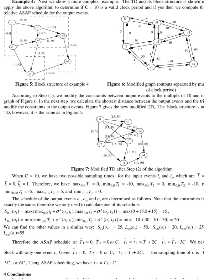
Example 4: Next we show a more complex example. The TD and its block structure is shown in figure 5. We apply the above algorithm to determine if C = 10 is a valid clock period and if yes then we compute the discrete-time relative ASAP schedule for the output events.

i1 i2 i3 o1 o2 o3 o4 [0,5] [15, 30] [15, 30] [1, 35] [1, 30] [-5, 5] [10, 60] [10, 60] [1, 80] [1, 50] i1 i2 i3 o1 o2 o3 o4 -15 5 ₀ 50 -10 60 -10 60 -1 -1 -10 -10 30 30 -15 30 30 80 0 0

Figure 5: Block structure of example 4 Figure 6: Modified graph (outputs separated by multiples of clock period)

According to Step (1), we modify the constraints between output events to the multiple of 10 and obtain the event graph of Figure 6. In the next step we calculate the shortest distance between the output events and the triggers and then modify the constraints to the output events. Figure 7 gives the new modified TD,. The block structure is not shown in the TD, however, it is the same as in Figure 5.

i1 i2 i3 o1 o2 o3 o4 [15, 30] [15, 30] [15, 30] [15, 30] [25, 60] [25, 60] [10, 60] [10, 60] [1, 35] [16, 50] [0, 5]

Figure 7: Modified TD after Step (2) of the algorithm

When C = 10, we have two possible sampling times for the input events i₁ and i₂, which are ~i1 =0,~i2 =0 and 1 ~ , 0 ~ 2 1 = i =

i . Therefore, we have max_0,0T = 0, ₁ min_0,0T = -10, ₁ max_0,0T = 0, ₂ min_0,0T = -10, ₂ max_0,10T = 0,₁

1 10 , 0

min T = -5, max_0,10T = 5, and ₂ min_0,10T = 0.₂

The schedule of the output events o₁, o2, and o3 are determined as follows. Note that the constraints for o1 and o2 are

exactly the same, therefore we only need to calculate one of its schedules.

15 } 15 0 , 15 0 max{ )} , ( max ), , ( max{max ) ( 1 0,0 1 1 1 0,0 2 1 2 0 , 0 o = i + o i i + o i = + + = S σs σs , 20 } 30 10 , 30 10 min{ )} , ( min ), , ( min{min ) ( 1 0,0 1 1 1 0,0 2 1 2 0 , 0 o = T + o i T + o i = − + − + = L σL σL

We can find the other values in a similar way: S_0,0(o₃) = 25, L_0,0(o₃) = 50, S_0,10(o₁) = 20, L_0,10(o₁) = 25, S_0,10(o₃) =3 0, L_0,10(o₃)=55.

Therefore the ASAP schedule is: T 0, T 0orC, t t T 2C t T1 3C

~ 3 ~ 1 ~ 2 ~ 1 ~ 2 ~ 1 ~ + = + = = =

= . We next consider the

block with only one event i3. Given 0, 0 or , 1 2 , ~ 2 ~ 2 ~ 1 ~ C T t C T

T = = = + the sampling time of i3 is 3

~

T = 3C , 4C, C

5 , or 6C, Using ASAP scheduling, we have t =T3+C

~ 4 ~

. 4 Conclusions

In this paper, a new way for scheduling events under real-time constraints and for the synthesis of interface controllers based on timing diagram specifications was described. The method allows to determine a valid clock period and is suitable for synchronous system implementations. An algorithm for deriving ASAP and ALAP relative schedules

for the output actions was presented for causal specifications. Expected applications of this method range from high-level synthesis to the synthesis of sampled-input synchronous interface controllers.

References

[1] M. McFarland, A. Parker, R. Camposano, "The high-level synthesis of digital systems", Proc. of the IEEE, No. 2, February 1990.

[2] G. Borriello, R. H. Katz, "Synthesizing transducers from interface specifications", VLSI’87, North Holland, 403-418, 1988.

[3] J. Brzozowski, T. Gahlinger, and F. Mavaddat, "Consistency and Satisfiability of Waveform Timing Specifications", Networks, Vol. 21, pp. 91-107, 1991.

[4] G. Borriello, "Formalized Timing Diagrams", Proc. Euro-DAC’92, pp. 372-377, 1992

[5] S. Lenk, "Extended Timing Diagrams as a specification language", Proc. Euro-DAC’94, pp.28-33, 1994. [6] R. Schlor, "A prover for VHDL-based hardware design", Proc. IFIP CHDL’95, 1995.

[7] K. McMillan and D. Dill, "Algorithms for interface timing verification", Proc. IEEE ICCD, 1992.

[8] E. Walkup, G. Borriello, "Interface Timing Verification with Application to Synthesis", Proc. DAC’94, 1994. [9] T. Yen, A Ishii, A. Casavant, W. Wolf, "Efficient Algorithms for interface timing verification", Euro-DAC, 1994. [10] G. De Micheli, Synthesis and Optimization of Digital Circuit, McGraw-Hill Inc. New York, 1994.

[11] W. Grass, C. Grobe, S. Lenk, and W. Tiedemann, "Timing diagrams as a specification language for interface circuits and their transformation into synchronous FSMs", BENEFIT-DMM 95. pp.280-35, Sept. 1995.

[12] W. Tiedemann, "An approach to multi-paradigm controller synthesis from timing diagram specifications", Euro-DAC’92, 1992.

[13] P. Gutberlet, W. Rosenstiel, "Interface Specification and Synthesis for VHDL Processes", Euro-DAC, 1993. [14] K. Khordoc, E. Cerny, "Modeling cell processing hardware with action diagrams", Proc. ISCAS’94, 1994.

[15] K. Khordoc, E. Cerny, “Semantics and Verification of Timing Diagrams with Linear Timing Constraints,” accepted to ACM Transactions on Design Automation of Electronic Systems (TODAES), May 1997, 25 p.

[16] P. Moeschler, H. Amann, F. Pellandini, "High-Level Modeling using Extended Timing Diagrams", Proc. Euro-VHDL '93, Hamburg, FRG, Sept. 1993, pp. 494-499.

[17] K. Khordoc, “Action Diagrams: A Methodology for the Specification and Verification of Real-Time Systems“, Ph.D. thesis, Dept. of Electrical and Computer Engineering, McGill University, March 1996.

[18] W-D. Tiedmann, "Introducing Clock Cycles", Report COPRODES/UPA/1995/2, University of Passau, Nov.1995. [19] B. Berkane, S. Gandrabur, E. Cerny, “Algebra of Communicating Timing Charts for Describing and Verifying

Hardware Interfaces,” Proc. IFIP Conf. on Computer Hardware Descr. Languages (CHDL’97), 1997.

[20] P. Girodias, E. Cerny, W.J. Older, “Solving Linear, Min and Max Constraint Systems Using CLP based on Relational Interval Arithmetic,” J. on Theor. Comp. Science, 173(2), Feb.97.

[21] P. Girodias, E. Cerny, “Interface Timing Verification with Delay Correlation Using Constraint Logic Programming,“ ED&TC’97

[22] D.C. Ku, G. De Micheli, “Relative Scheduling under Timing Constraints: Algorithm for High-Level Synthesis of Digital Circuits,” IEEE Trans. CAD ICS, 11(6), June 1992, pp. 696-718.