Using CloudSat observations to evaluate cloud top heights from convection parameterization. © 2017 Guang Jun Zhang and Mingcheng Wang. This is an Open Access article distributed under the terms of the Creative Commons Attribution-NonCommercial 4.0 International License (http://creativecommons.
Using CloudSat observations to evaluate cloud top
heights from convection parameterization
Guang Jun Zhang
1, 2*and Mingcheng Wang
11 Department of Earth System Science, Tsinghua University, Beijing, China 2 Scripps Institution of Oceanography, La Jolla, California, USA
Abstract: How high convective clouds can go is of great importance to climate. Cloud ice and liquid water that detrain near the top of convective cores are important for the formation of anvil clouds and thus impact cloud radiative forcing and the Earth’s radiation budget. This study uses CloudSat observations to evaluate convective cloud top heights in the National Center for Atmospheric Research (NCAR) Community Atmosphere Model (CAM5). Results show that convective cloud top heights in the tropics are much lower than observed by CloudSat, by more than 2 km on average. Temperature and moisture anomalies from climatological means are composited for convective clouds of different heights for both observations and model simulation. It is found that convective environment is warmer and moister, and the anomalies are larger for clouds of higher tops. For a given convective cloud top height, the corresponding atmosphere in CAM5 is more convectively unstable than what the CloudSat observations indicate, suggesting that there is too much entrainment into convective clouds in the model.
Keywords: CloudSat; cloud top heights; satellite data
*Correspondence to: Guang Jun Zhang, Scripps Institution of Oceanography, La Jolla, California, USA; Email: [email protected] Received: August 25, 2017; Accepted: October 25, 2017; Published Online: November 15, 2017
Citation: Zhang G J, Wang M. (2017). Using CloudSat observations to evaluate cloud top heights from convection parameterization.
Satellite Oceanography and Meteorology, 2(2): 298. http://dx.doi.org/10.18063/SOM.v2i2.298
1. Introduction
S
atellite data have been used widely for weather and climate research since its inception. The Earth Radiation Budget Experiment (ERBE), which used multiple satellites launched in 1984 from NASA and NOAA for Earth’s radiation measurement was the first extensive use of satellite observations for climate research (Ramanathan et al., 1989). It provided a comprehensive estimate of cloud radiative effect on the Earth system. Later use of other satellite data including the International Satellite Cloud Climatology Project (ISCCP, Rossow and Schiffer 1991, 1999), Clouds and the Earth’s Radiant Energy System (CERES, Wiellickiet al., 1996) onboard the Tropical Rainfall Measurement Mission (TRMM, Simpson et al., 1996) have all proven to be extremely valuable for understanding of the Earth’s climate system, and for evaluating and improving global climate models (GCM). For instance, CERES and ISCCP cloud observations have been used extensively for evaluating global cloud distribution and cloud properties (Pincus et al., 2008; Klein et al., 2013).
More recently, the CloudSat mission (Stephens et al., 2002) provided vertical structure information of clouds
that can be used to compare with model-simulated clouds. CloudSat observations have since been used extensively for GCM evaluation of cloud properties and precipitation (Waliser et al., 2009; Stephens et al., 2010; Jiang et al., 2012; Li et al., 2012; Su et al., 2013). Su et al. (2013) showed that in all Climate Model Intercomparison Project Phase 5 (CMIP5) models the vertical structure of high and low clouds and their relationship with large-scale fields differ significantly from observations, and cloud parameterization errors dominate the total error. Li et al. (2012) showed that cloud ice water path simulated by most CMIP5 models differs from CloudSat observations by a factor of 2 to 10, highlighting the challenges GCMs face to get the ice cloud right.
Convective cloud top heights (CTH) are of particular importance to climate and climate change. The de train-ment of ice and liquid water from convective updraft cores is a major source for anvil clouds (Gamache and Houze, 1983; Ramanathan and Collins, 1991). Since most of the detrainments occur near the convective cloud top where updraft air loses its buoyancy, CTH can directly affect the Earth’s radiation budget and thus climate.
of studies recently to document convective cloud characteristics, including CTH, effective entrainment rate in convection, and the level of neutral buoyancy and convective outflow (Luo et al., 2008, 2010; Meenu
et al., 2010; Takahashi and Luo, 2012; Takahashi
et al., 2017). Luo et al. (2008) documented the characteristics of convective cloud top at different stages of convection development. Meenu et al. (2010) examined the regional differences in CTHs over the Indian subcontinent and surrounding oceans. Takahashi and Luo (2012) and Takahashi et al. (2017) examined the relationships among neutral buoyancy level (NBL), level of convective outflow and convective core, and their dependence on environmental thermodynamic conditions and convective system size. Such information is valuable for evaluating convection parameterization in GCMs. Surprisingly, although CTH is diagnosed in all convective parameterization schemes, as far as the authors are aware, little has been done to evaluate the simulation of convective CTHs and their relationships with the environmental conditions against observations despite its importance in climate.
Motivated by these observational studies using CloudSat data, this study aims to use the observed convective CTHs to evaluate the convection pa ram e ter-iza tion scheme in the National Center for Atmospheric Research (NCAR) Community Atmosphere Model version 5 (CAM5).
2. Data, Model Simulation and Analysis
Method
CloudSat was launched in April 2006. Due to large volume of data, only four years of CloudSat data (June 2006 to May 2010) are analyzed in this study. The nadir-looking cloud profiling radar (CPR) has a frequency of 94 GHz with a sensitivity of −30 dBZ. The data have a horizontal resolution of 1.7 km along track and 1.4 km cross crack. The vertical resolution is 480 m (Stephens et al., 2008) with 240-m oversampling intervals. The main data product used in this study is the 2B-GEOPROF (Mace et al., 2007) cloud mask and radar reflectivity
The NCAR CAM5 is used for model simulation of convection. The model-simulated convective CTHs are then analyzed for evaluation and comparison with the CloudSat data. The CAM5 (Neale et al., 2008) has a horizontal resolution of 1.9° × 2.5° with 30 vertical levels. Deep convection is parameterized by the Zhang-McFarlane (ZM) scheme (Zhang and Zhang-McFarlane, 1995), with modification by Neale et al. (2008) to account for convective available potential energy (CAPE) dilution by entrainment. Shallow convection and planetary boundary layer are parameterized following Park and Bretherton (2009) and Bretherton and Park (2009), respectively. The large-scale microphysics is parameterized using the two-moment microphysics scheme of Morrison and Gettelman (2008).
The CAM5 simulation covering the same time period as that for CloudSat observations used in this study is performed. The model simulation starts on June 1 2005 and run through May 2010 with the first-year data discarded for model spin-up. The instantaneous output for convection-related variables such as NBL, convective mass flux, detrainment and associated grid point temperature and moisture profiles is saved at hourly frequency. In the ZM scheme used in CAM5, entrainment dilution is considered in CAPE calculation according to Neale et al. (2008) with an entrainment rate that doubles convective mass flux every kilometer. The NBL determined during the CAPE calculation is assumed to be the convective CTH. For CloudSat observations, we determine convective CTH following the work of Luo et al. (2008) and Takahashi and Luo (2012, 2017). First, deep convection is identified in a CloudSat radar profile cross-section along the satellite path if the following criteria are satisfied: (1) the cloud top ≥ 6 km, (2) cloud-base height ≤ 2km, (3) radar echo from base to top is continuous, and (4) the cloud mask is ≥ 20, which means a high confidence in cloud detection (Marchand et al., 2008). The highest echo top within each identified cloud object is considered the CTH. Figure 1 shows an example of convective clouds containing convective cores, cloud top and base
heights so determined. For CAM5, deep convective cloud is defined by (1) the CTH determined by the ZM scheme is ≥ 6km and (2) the parcel lifting level, which is considered to be convective cloud base, is ≤ 2km.
3. Results
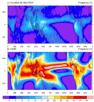
One of the basic statistics of convection is its frequency of occurrence. The occurrence frequency of deep convection during the 4-year observations and model
simulation period is calculated and shown in Figure 2 for cloud tops above 6 km. In the CloudSat observations, the frequency of deep convection at a given location is obtained by dividing the number of samples identified as deep convection by the total number of samples during the entire observation period analyzed. Similarly, for CAM5 simulation the frequency of deep convection at a given GCM grid point is calculated as the ratio of the number of output samples when deep convection (i.e. Figure 1. Vertical cross section of cloud profiling radar reflectivity of clouds
detected by CloudSat along the satellite track. The black line marks deep convective cloud top heights.
Figure 2. Frequency of convection with tops above 6 km in (A) CloudSat observations and (B) CAM5 simulation averaged over four years.
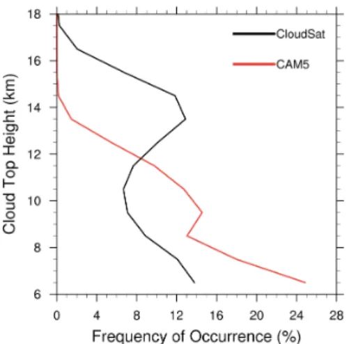
Figure 3. Frequency of occurrence of deep convection with tops
at different heights for CloudSat (black) and CAM5 (red) averaged
between 30°N. deep convection over the tropical belt (30°S, 30°N) is
4.85% in CloudSat observations vs. 17.52% in CAM5. This hyperactive behavior of convection in the NCAR GCM as well as other numerical weather prediction and global climate models is well known (e.g. Dai and Trenberth 2004, Stephens et al., 2010), and is believed to be one of the factors responsible for the poor simulation of intraseasonal variability in the model (Lin et al., 2006).
Although deep convection occurs more frequently in CAM5, the CTHs are much lower than observed in CloudSat. Figure 3 shows the relative frequency of occurrence of CTHs in CloudSat and CAM5 in the (30°S, 30°N) belt when deep convection with tops above 6 km does occur. The values for CTHs are binned at 1-km interval and the midpoints of the intervals (e.g.
6.5 km, 7.5 km, etc.) are used to represent CTHs. The CloudSat data show a bimodal distribution from 6 km to 18 km, with one peak at 13.5 km and the other at 6.5 km, and a minimum at 10.5 km. On the other hand, CAM5 systematically underestimates convection top by more than 2 km. CAM5 CTHs vary from 6.5 km to 14.5 km with two peaks at 9.5 km and 6.5 km, and a minimum at 8.5 km, respectively. Although there is also a bimodal distribution, the minimum frequency layer is quite shallow, and there is more abundance of shallower convection below 8 km. The average CTH for CloudSat is 11 km vs. 8.6 km in CAM5. This clearly shows that convective CTHs are seriously underestimated in CAM5.
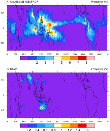
To further demonstrate this point, Figure 4 shows the frequency of occurrence of deep convection with tops reaching 14 km in CloudSat and CAM5. Note that in order to make the plot visually more noticeable, the color scale for CAM5 is reduced by a factor of 5. In CloudSat, convection can reach 14 km height in the broad tropical region including the Pacific and Atlantic ITCZ, Indian Ocean and the tropical land areas, whereas in CAM5, it only occurs in very limited areas in the western Pacific warm pool, Indian monsoon and northwestern Australia.
How high convective clouds can go is of fundamental
importance to climate. Cloud ice and liquid water that detrain near the cloud top are important sources for cirrus/anvil clouds and thus impact cloud radiative forcing (Ramanathan and Collins, 1991, Bony et al., 2016). Here we use CAM5 output to demonstrate this point. Figure 5 shows the probability distribution functions of longwave cloud radiative forcing (LWCF) corresponding to convective clouds of different top heights and their mean values. For lower cloud tops (e.g. tops lower than 9 km), most of the LWCF is less than 80 W/m2. As CTH increases, the maximum probability
shifts toward higher values. For instance, CTHs in the range of 13 – 14 km have a maximum probability at 130 W/m2. The average LWCF for each CTH also increases
as clouds become deeper although not monotonically. This is because cloud radiative forcing in a GCM grid box depends on cloud properties in the entire grid box and the top of convective clouds is only one of the contributing factors.
Convection develops when the atmospheric en vi ron-ment is favorable. Thus, it is expected that convection with tops reaching different heights will likely correspond to different environmental thermodynamic conditions. To examine this, the collocated ECMWF-AUX dataset is combined with the CloudSat CPR data to obtain composite vertical profiles of temperature anomalies from the climatological mean for CloudSat and CAM5, respectively (Figure 6). For CloudSat, the climatological mean is obtained by averaging all profiles, including both cloudy and clear scenes, within (30°S, 30°N) along the satellite path. For CAM5, the climatological mean is the spatial and temporal average in the (30°S, 30°N) belt. Clearly, convection develops in a warmer environment compared to climatological means, with positive temperature anomalies of up to 2 to 3 K. Shallower convection corresponds to smaller
peaking at 16.5 km. This indicates that the tropopause is colder when there is deep convection. The temperature anomalies are larger for deeper convection. The CAM5 model simulation shows similar behavior, but with about twice as large anomalies for both positive and negative values, an indication that the CAM5 atmosphere is more unstable.
anoma lies. Interestingly, for all clouds there is a min i-mum anomaly near the 4-km height. It is possible that the minimum reflects the effect of melting of ice in clouds at the freezing level, which is around 4 km in the tropics. Temperature anomalies reach maximum in the upper troposphere around 10 km. There is a layer of large negative anomalies above 13.5 km for all clouds,
Figure 4. Frequency of deep convection with tops above 14 km for (A) CloudSat and (B) CAM5. Note that the color scale has been reduced by a factor of 5 in (B) for visual convenience.
Figure 5. (A) Probability distribution function of longwave cloud radiative forcing for
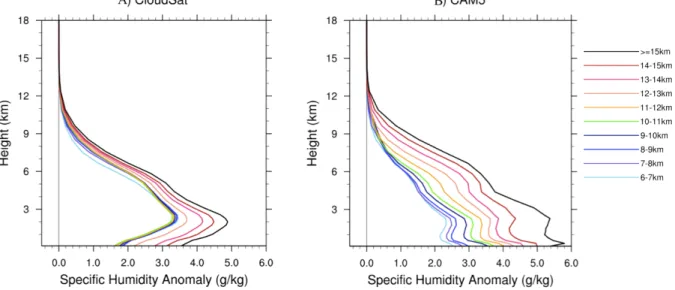
Figure 7 shows the specific humidity anomalies from CloudSat observations and CAM5 simulation. The entire troposphere is moister than the climatological mean, with a peak near 2 km for all clouds. For convection tops less than 11 km, the moisture anomalies have little dependence on CTH, whereas for cloud tops higher than 11 km the moisture anomalies increase with CTHs, reaching as high as 5 g/kg at 2 km for cloud tops higher than 15 km. For CAM5, the atmosphere is also moister throughout the troposphere than the climatological mean. However, there are two distinct differences from the CloudSat observations. First, moisture anomalies increase monotonically with CTH, even for clouds with tops less than 11 km high. Second, the anomalies
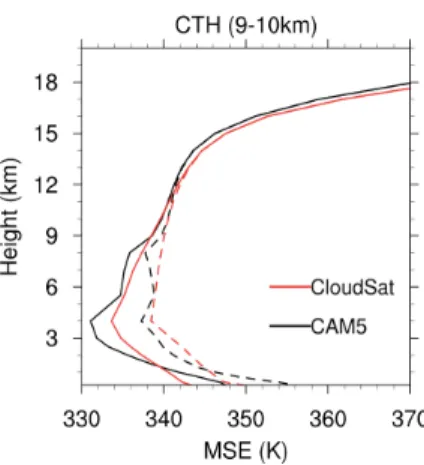
for a given CTH reach a maximum at the surface, although a secondary maximum at 2 km is visible. This again indicates that the boundary layer air in CAM5 is thermodynamically more unstable in the tropical convection regime. To verify this, we plot the composite profiles of moist static energy and its saturation value (divided by atmospheric heat capacity at constant pressure Cp) sampled for CTHs between 9 and 10 km in
Figure 8. Results are similar for other CTHs. Both the CloudSat-observed atmosphere and CAM5-simulated atmosphere are convectively unstable, more so for the CAM5-simulated atmosphere. The surface moist static energy in the CAM5 simulation is about 2 K higher than that in CloudSat observations. For an undiluted
Figure 6. Composite temperature anomalies from climatological mean for deep convective environment with different cloud top heights
for (A) CloudSat observations and (B) CAM5 simulation between 30°S and 30°N.
Figure 7. Composite temperature anomalies from climatological mean for specific humidity for (A) CloudSat observations and (B) CAM5 simulation between 30°S and 30°N.
Figure 8. Profiles of composite moist static energy (solid line) and
its saturation value (dashed line) for convective clouds with tops between 9 and 10 km height between 30°S and 30°N.
air parcel, its moist static energy does not change with height as it rises in the convective cloud. Thus, for the observed atmosphere, an undiluted air parcel from the most unstable level near the surface can reach 13 km, whereas for the CAM5 atmosphere, it can reach as high as 15.5 km. Since the actual convection in both CloudSat data and CAM5 reaches 9 – 10 km, this suggests that there is too much entrainment in CAM5 compared to what CloudSat data implies.
that deep convection occurs in a warmer and moister environment compared to climatological means. CAM5 is able to simulate this well. However, maximum moisture anomalies are observed in CloudSat at 2 km whereas it occurs at the surface in CAM5 for all convective clouds deeper than 6 km. Also, temperature anomalies in CAM5 are about twice as large as in the observations. Composite moist static energy profiles show that for convection reaching the same CTHs, the CAM5 atmosphere is much more unstable than in observations. This implies that entrainment dilution in the model is too strong. Since convection top in CAM5 is set by the NBL in the dilute CAPE calculation with a prescribed entrainment rate (Neale et al., 2008), retuning of this parameter is necessary to increase CTHs in the model.
Conflict of Interest
No conflict of interest was reported by the authors.
Acknowledgments
This work is supported by the National Key R&D Program of China 2017YFA0604000, the U.S. National Science Foundation Grant AGS-1549259, and the U.S. Department of Energy, Office of Science, Biological and Environmental Research Program (BER), under Award Number DE-SC0016504. The authors thank the anonymous reviewers for their constructive comments.
References
Bacmeister J T and Stephens G L. (2011). Spatial statistics of likely convective clouds in CloudSat data. Journal of Geophysical Research, 116(D4): D04104.
http://dx.doi.org/10.1029/2010jd014444
Betts A K. (1990). Greenhouse warming and the tropical water budget. Bulletin of the American Meteorological Society, 71(10): 1464–1465.
Bony S, Stevens B, Coppin D, et al. (2016). Thermodynamic control of anvil cloud amount. Proceedings of the National Academy of Sciences, 113(32): 8927–8932.
http://dx.doi.org/10.1073/pnas.1601472113
Bretherton C S and Park S. (2009). A new moist turbulence parameterization in the community atmosphere model. Journal of Climate, 22(12): 3422–3448.
http://dx.doi.org/10.1175/2008jcli2556.1
Dai A and Trenberth K E. (2004). The diurnal cycle and its depiction in the Community Climate System Model. Journal of Climate, 17: 930–951.
http://dx.doi.org/10.1175/1520-0442(2004)017<0930:TDCAI
4. Summary
This study analyzed the CPR data from CloudSat to estimate convective CTHs for deep convection reaching 6 km or higher. These estimates are then used to compare with the NCAR CAM5 model simulation. Collocated ECMWF Reanalyses data for environmental conditions of convection through the auxiliary dataset ECMWF-AUX are also analyzed. It is found that convective CTHs in CAM5 are systematically lower than CloudSat observations by more than 2 km. Observed convection tops can reach 17 km in the tropics while model convection can seldom reach 14 km. The average convective CTH in the CloudSat data in the tropical region (30°S, 30°N)is 11 km, compared to 8.6 km in CAM5 in the same region. The grid box means longwave cloud radiative forcing in CAM5 is found to increase with convective CTH. This is presumably due to detrainment of cloud ice and liquid water from convective cores into anvil clouds associated with con-vec tive systems. The higher the concon-vective top, the higher the detrainment level, thus the larger the cloud radiative effect would be. Therefore, the underestimation of convective CTHs in CAM5 can have important ramifications on the simulated radiative energy budget in the model.
Combined analysis of convective top heights and thermodynamic fields (temperature and moisture) shows
Klein S A, Zhang Y, Zelinka M D, et al. (2013).Are climate model simulations of clouds improving? An evaluation using the ISCCP simulator. Journal of Geophysical Research, 118(3): 1329–1342.
http://dx.doi.org/10.1002/jgrd.50141
Li J-L F, Walliser D E, Chen W T, et al. (2012). An observationally based evaluation of cloud ice water in CMIP3 and CMIP5 GCMs and contemporary reanalyses using contemporary satellite data. Journal of Geophysical Research,117(D16): D16105.
http://dx.doi.org/10.1029/2012JD017640
Lin J-L, Kiladis G N, Mapes B E, et al. (2006). Tropical intraseasonal variability in 14 IPCC AR4 Climate Models. Part I: Convective signals. Journal of Climate, 19: 2665–2690.
http://dx.doi.org/10.1175/JCLI3735.1
Lindzen R S. (1990). Some coolness concerning global warming. Bulletin of the American Meteorological Society, 71(3): 288– 299.
http://dx.doi.org/10.1175/1520-0477(1990)071<0288:SCCG W>2.0.CO;2
Luo Z, Liu G Y and Stephens G L. (2008). CloudSat adding new insight into tropical penetrating convection. Geophysical Research Letters, 35(19): L19819.
http://dx.doi.org/10.1029/2008GL035330
Luo Z J, Liu G Y and Stephens G L. (2010). Use of A-Train data to estimate convective buoyancy and entrainment rate. Geophysical Research Letters, 37(9): L09804.
http://dx.doi.org/10.1029/2010GL042904
Mace G G, Marchand R, Zhang Q, et al. (2007). Global
hydrometeor occurrence as observed by CloudSat: Initial
observations from summer 2006. Geophysical Research
Letters, 34(9): L09808.
http://dx.doi.org/10.1029/2006GL029017
Marchand R, Mace G G, Ackerman T, et al. (2008). Hydrometeor detection using Cloudsat—An Earth-orbiting 94-GHz cloud
numerical tests. Journal of Climate, 21: 3642–3659. http://dx.doi.org/10.1175/2008jcli2105.1
Neale R B, Richter J H and Jochum M. (2008). The impact of convection on ENSO: From a delayed oscillator to a series of events. Journal of Climate, 21: 5904–5924.
http://dx.doi.org/10.1175/2008jcli2244.1
Park S and Bretherton C S. (2009). The University of Washington shallow convection and moist turbulence schemes and their impact on climate simulations with the community atmosphere model. Journal of Climate, 22: 3449–3469.
http://dx.doi.org/10.1175/2008jcli2557.1
Partain P. (2004). Cloudsat ECMWF-AUX auxiliary data process description and interface control document. Colorado: Colorado State University; [updated 2004 July 30; cited 2017 July 30] Available from:
http://cswww.cira.colostate.edu/ICD/ECMWF-AUX/ ECMWF-AUX_PDICD_3.0.pdf
Pincus R, Batstone C P, Hofmann R J P, et al. (2008). Evaluating the present-day simulation of clouds, precipitation, and radiation in climate models. Journal of Geophysical Research, 113(D14): D14209.
http://dx.doi.org/10.1029/2007JD009334
Ramanathan V, Cess R D, Harrison E F, et al. (1989). Cloud-radiative forcing and climate: Results from the Earth radiation budget experiment. Science, 243(4887): 57–63.
https://doi.org/10.1126/science.243.4887.57
Ramanathan V and Collins W. (1991). Thermodynamic regulation of ocean warming by cirrus clouds deduced from observations of the 1987 El Niño. Nature, 351: 27–32.
http://dx.doi.org/10.1038/351027a0
Rossow W B and Schiffer R A. (1991). ISCCP cloud data products. Bulletin of the American Meteorological Society, 72(1): 2–20.
https://doi.org/10.1175/1520-0477(1991)072<0002:ICDP>2.0 .CO;2
Rossow W B and Schiffer R A. (1999). Advances in understanding
clouds from ISCCP. Bulletin of the American Meteorological Society, 80(11): 2261–2287.
https://doi.org/10.1175/1520-0477(1999)080<2261:AIUCFI> 2.0.CO;2
Simpson J, Kummerow C, Tao W K, et al. (1996). On the Tropical Rainfall Measuring Mission (TRMM). Meteorology and Atmospheric Physics, 60(1–3): 19–36.
http://dx.doi.org/10.1007/BF01029783
Stephens G L, L'Ecuyer T, Forbes R, et al. (2010). Dreary state of precipitation in global models. Journal of Geophysical Research,115(D24): D24211.
http://dx.doi.org/10.1029/2010JD014532
Stephens G L, Vane D G, Boain R J, et al. (2002). The CloudSat Mission and the A-Train, A new dimension of space-based observations of clouds and precipitation. Bulletin of the American Meteorological Society, 83: 1771–1790.
http://dx.doi.org/10.1175/BAMS-83-12-1771
Su H, Jiang J H, Zhai C, et al. (2013). Diagnosis of regime-dependent cloud simulation errors in CMIP5 models using “A-Train” satellite observations and reanalysis data. Journal of Geophysical Research Atmospheres, 118(7): 2762–2780. http://dx.doi.org/10.1029/2012JD018575
Takahashi H and Luo Z. (2012). Where is the level of neutral
buoyancy for deep convection? Geophysical Research Letters, 39(15): L15809.
http://dx.doi.org/10.1029/2012GL052638
Takahashi H, Luo Z J and Stephens G L. (2017). Level of neutral
buoyancy, deep convective outflow and convective core: New
perspectives based on 5-years of CloudSat data. Journal of Geophysical Research Atmospheres, 122(5): 2958–2969.
http://dx.doi.org/10.1002/ 2016JD025969
Waliser D E, Li J-L F., Woods C P, et al. (2009).Cloud ice: A climate model challenge with signs and expectations of progress. Journal of Geophysical Research Atmospheres,
114(D8): D00A21.
http://dx.doi.org/10.1029/2008JD010015
Wielicki B A, Barkstrom B R, Harrison E F, et al. (1996). Clouds and the Earth’s Radiant Energy System (CERES): An earth
observing system experiment. Bulletin of the American
Meteorological Society, 77(5): 853–868.
https://doi.org/10.1175/1520-0477(1996)077<0853:CATERE >2.0.CO;2
Zhang G J and McFarlane N A. (1995). Sensitivity of climate simulations to the parameterization of cumulus convection in the Canadian Climate Centre general circulation model. Atmosphere-Ocean, 33(3): 407–446.