An Approach to Task-based Parallel Programming for
Undergraduate Students
Eduard Ayguad´ea,b,∗, Daniel Jim´enez-Gonz´aleza,b
aComputer Architecture Department, Universitat Polit`ecnica de Catalunya (UPC) bComputer Sciences Department, Barcelona Supercomputing Center (BSC-CNS)
Abstract
This paper presents the description of a compulsory parallel programming course
in the bachelor degree in Informatics Engineering at the Barcelona School of
In-formatics, Universitat Polit`ecnica de Catalunya UPC–BarcelonaTech. The main
focus of the course is on the shared-memory programming paradigm, which
fa-cilitates the presentation of fundamental aspects and notions of parallel
com-puting. Unlike the “traditional” loop-based approach, which is the focus of
par-allel programming courses in other universities, this course presents the parpar-allel
programming concepts using a task-based approach. Tasking allows students
to explore a broader set of parallel decomposition strategies, including linear, iterative and recursive strategies, and their implementation using the current
version of OpenMP (OpenMP 4.5), which offers mechanisms (pragmas and
in-trinsic functions) to easily map these strategies into parallel programs. Simple
models to understand the benefits of a task decomposition and the trade-offs
introduced by different kinds of overheads are included in the course, together
with the use of tools that allow an easy exploration of different task
decompo-sition strategies and their potential parallelism (Tareador) and instrumentation
and analysis of task parallel executions on real machines (Extrae andParaver).
Keywords: Task decomposition strategies and programming, OpenMP
tasking model, Performance models and tools
∗Corresponding author
1. Introduction 1
For decades, single-core processors were steadily improving in performance 2
thanks to advances in integration technologies (bringing more transistors and 3
ever-increasing clock speeds) and micro-architectural innovations (providing high-4
er potential instruction-level parallelism, or ILP). The target’s ILP could be 5
satisfactorily exploited by the compiler, and sequential programming was the 6
dominant paradigm. Programming courses for undergraduate students were 7
based on this sequential paradigm, without the need for programmers to learn 8
to consider parallelism. Concurrency was mainly presented in operating system 9
(OS) courses as a way to express the concurrent execution of multiple activi-10
ties, such as processes and/or threads, inside the OS. Parallel computing was a 11
subject mainly considered in courses at the most advanced levels of computer 12
science and engineering curricula. 13
This sequential paradigm was challenged by the move towards multicore 14
architectures, caused by the power wall (due to ever-increasing clock frequencies) 15
and increasing difficulties in exploiting the available ILP. Today, from mobile to 16
desktops to laptops to servers, multicore processors and multiprocessor systems 17
are commonplace. In order to utilise the increasing number of available cores, 18
it is necessary to parallelise existing sequential applications. Unfortunately, 19
neither hardware nor current compilers can automatically detect and exploit 20
the levels of parallelism required to feed current parallel architectures. 21
Due to the increasing demand in the IT sector for parallel programming ex-22
pertise, efforts have been made to introduce parallel programming to undergrad-23
uate students. In most cases the design of these parallel programming courses 24
stayed rooted in “traditional” regular loop-level parallelisation strategies, not 25
allowing parallelism to be exploited in more irregular applications, such as those 26
traversing dynamically-allocated data structures (lists, trees, etc.) and making 27
use of other control structures, such as recursion. In addition, it has been proven, 28
both by the research community and through the evolution of parallel program-29
ming standards, that this “traditional” approach is not sufficient to pave the 30
path towards exploiting the potential scalability of future processor generations 31
and architectures. To provide an alternative to the loop-based approach, some 32
programming models and standards (such as OpenMP) evolved to include the 33
tasking model. The task-based approach offers a means to express irregular 34
parallelism, in a top down manner, that scales to large numbers of processors. 35
In this paper we present the proposed syllabus and framework for teaching 36
parallel programming to “fresh” students inParallelism, a third-year compul-37
sory subject in the Bachelor Degree in Informatics Engineering at the Barcelona 38
School of Informatics (FIB) of the Universitat Polit`ecnica de Catalunya (UPC– 39
BarcelonaTech). This subject has been our first opportunity to teach parallelism 40
at the undergraduate level. The tasking model in OpenMP [1] (currently version 41
4.5 for C/C++) was chosen as the vertebral axis in the design of this course, 42
providing support for tasks (including task dependences) in addition to tradi-43
tional loop-level parallelism, which is considered to be a particular case of the 44
generic tasking model. The course also includes models and tools to understand 45
the potential of task decomposition strategies (Tareador [2]) as well as to un-46
derstand their actual behaviour when expressed in OpenMP and executed on 47
a real parallel architecture (Extrae, a dynamic tracing package, andParaver, a 48
trace visualisation and analysis tool [3]). The complete framework motivates 49
the learning process, improves the understanding of the proposed task decom-50
positions and significantly reduces the time to develop parallel implementations 51
of the original sequential codes. 52
The paper is organised as follows: Section 2 presents the context for the 53
subject presented in this paper. Then, Sections 3, 4, 5 and 6 describe the main 54
units in the subject, in terms of concepts and methodology. Finally, Section 7 55
concludes the paper by analysing how the proposed subject covers the main 56
topics identified in theNSF/IEEE-TCPP Curriculum Initiative on Parallel and
57
Distributed Computing - Core Topics for Undergraduates, and how the grad-58
ual evolution from a traditional loop-based course has improved the students’ 59
results. 60
2. Course description and context 61
The bachelor degree in Informatics Engineering at the Barcelona School 62
of Informatics of the Universitat Polit`ecnica de Catalunya is designed to be 63
completed in seven terms (two terms per academic year) plus one term for a 64
final project. The four initial terms cover subjects that are mandatory for all 65
students, while the three final terms comprise mandatory and elective courses 66
within one specialisation (computer engineering, networks, computer sciences 67
and software engineering). 68
Parallelism (PAR) is the first subject in the above-mentioned degree that 69
teaches parallelism, and it is the one described in detail in this paper. It is 70
a compulsory subject, in the fifth term, that covers parallel programming and 71
parallel computer architecture fundamentals—basic tools to take advantage of 72
the multi-core architectures that constitute today’s computers. The subject 73
follows a series of subjects on computer organisation and architecture, operating 74
systems, programming and data structures, all of which are focussed on uni-75
processor architectures and sequential programming. 76
2.1. Learning objectives and student learning outcomes
77
The three main learning objectives of PAR are the following: (1) to design, 78
implement and analyse parallel programs for shared-memory parallel architec-79
tures; (2) to write simple models to evaluate different parallelisation strategies 80
and understand the trade-off between parallelism and the overheads of paral-81
lelism; and (3) to gain an understanding of the architectural support for parallel 82
programming models (data sharing and synchronisation). 83
The expected student learning outcomes for PAR are summarised in Fig-84
ure 1; these learning outcomes are related to the different theory/laboratory 85
sessions shown in Table 1 and described in the next subsection. 86
2.2. Complementary courses
87
Two elective subjects in the specialisation of Computer Engineering fol-88
low PAR. First, Parallel Architectures and Programming (PAP) extends the 89
Figure 1: Student’s Learning Outcomes (LO) for PAR.
concepts and methodologies introduced in PAR, by focussing on the low-level 90
aspects of implementing a programming model such as OpenMP, making use 91
of low-level threading (Pthreads); the subject also covers cluster architectures 92
and how to program them using MPI. Second,Graphical Units and Accelerators
93
(TGA) explores the use of accelerators, with an emphasis on GPUs, to exploit 94
data-level parallelism. 95
PAR, PAP and TGA are complemented by a compulsory course in the Com-96
puter Engineering specialisation,Multiprocessor Architectures, in which the ar-97
chitecture of (mainly shared-memory) multiprocessor architectures is covered in 98
detail. Another elective subject in the same specialisation, Architecture-aware
99
Programming (PCA), mainly covers programming techniques for reducing the 100
execution time of sequential applications, including through SIMD vectorisation 101
and FPGA acceleration. 102
Theory/problem solving Laboratory Learning
Week Topic Session (2h) Topic Session (2h) Outcomes (LO)
1 Fundamentals Motivation. Serial, multiprogrammed, Environment Compilation and LO1,4
concurrent and parallel execution execution of programs
2 Abstract program representation (TDG). Tools: Tareador LO1
Simple performance models and overheads.
3 Amdahl’s law. Strong vs. weak scalability Tools: Paraver and Extrae LO2,5,6
4 Wrap-up and exercises OpenMP Parallel and work–sharing LO1,2
5 Task Linear, iterative and recursive. Task granularities. tutorial Tasking execution model LO3
6 decomposition Task ordering vs. data sharing constraints Model analysis Evaluation of overheads LO3,6
7 Wrap-up and exercises Embarrassingly Design LO1,3
8 More advanced exercises covering decomposition strategies Parallel Implementation LO1-6
and task ordering / data sharing constraints and analysis
9 1st Midterm Evaluation
10 Architecture support How data is shared among processors? Divide and Design LO1,3,7,8
11 for shared memory How are processors able to synchronise? conquer Implementation LO3
12 programming Wrap-up and exercises Analysis LO1,3,7,8
13 Data Strategies to improve data locality: think about Geometric Design LO1,3
decomposition data. Owner-computes rule decomposition
14 Why sharing data? Distributed memory and MPI Implementation LO8
15 Wrap-up and exercises Analysis LO1,3,7,8
2nd Midterm Evaluation
2.3. Course outline
103
Each term effectively lasts for 15 weeks. In PAR there are four contact hours 104
per week: two hours devoted to theory and problems (with a maximum of 60 105
students per class) and two hours for laboratory sessions (with a maximum of 15 106
students per class). Students are expected to invest about six additional hours 107
per week to complete homework and for personal study (over these 15 weeks). 108
Thus, the total effort devoted to the subject is six ECTS credits.1 109
Table 1 shows the main contents of PAR and their weekly distribution in 110
theory/problem and laboratory sessions. After an introductory unit motivating 111
the course and presenting the differences between sequential, multiprogrammed, 112
concurrent and parallel execution, PAR continues with four units that cover the 113
objectives of the course: fundamentals of parallelism (described in Section 3), 114
task decomposition strategies (described in Section 4), introduction to parallel 115
computer architectures (described in Section 5) and data decomposition strate-116
gies (described in Section 6). 117
Theory/problem contact classes follow the flipped classroom methodology: 118
before class students complete one or more interactive learning modules that 119
include videos explaining the main concepts, and during the class students ap-120
ply the key concepts and extend them to more complex concepts. Finally, after 121
class, students check their understanding and extend their learning to more 122
complex tasks. In addition, there are several wrap-up sessions to help the learn-123
ing process, and there are two midterm exams. As shown in Table 1, several 124
laboratory sessions are coordinated with the theory and problem contact classes. 125
The structure of the course and some of its main concepts are based on 126
two books: Patterns for Parallel Programming [4] and Introduction to Parallel
127
Computing [5]. The latest OpenMP specification [1] is also used as reference 128
1The European Credit Transfer System (ECTS) is a unit of appraisal of the academic ac-tivity of the student. It takes into account student attendance at lectures and time of personal study, exercises, labs and assignments, together with the time needed to do examinations. One ECTS credit is equivalent to 25–30 hours of student work.
material. Finally, Computer Architecture: a Quantitative Approach [6] is rec-129
ommended as complementary material. 130
3. The fundamentals 131
After introducing the differences between serial, multiprogrammed, con-132
current and parallel execution, the subject starts by presenting an abstract 133
representation for task-based parallelisation strategies: the task dependence
134
graph (TDG), which allows an analysis of the parallelism of a particular de-135
composition into tasks. The TDG is a directed acyclic graph in which each 136
node represents a task, which is an arbitrary sequential computation, and each 137
directed edge represents a data dependence relationship between the predeces-138
sor and successor tasks. The weight of a node represents the amount of work to 139
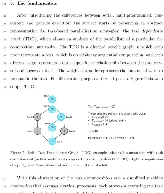
be done in the task. For illustration purposes, the left part of Figure 2 shows a 140 simple TDG. 141 10 10 2 2 5 10 5 3 Task A Task B Task C Task E Task D Task F Task G Task H T1= T{ABCDEFGH}= 47
Three possible paths in the graph, with costs • T{ABCEH}= 29
• T{ABDFH}= 40 (critical path)
• T{ABDGH}= 33
T∞= 40
Parallelism = T1/ T∞ =47/40 = 1.175.
Figure 2: Left: Task Dependence Graph (TDG) example, with nodes annotated with task execution cost (in blue nodes that compose the critical path in the TDG). Right: computation ofT1,T∞andParallelismmetrics for the TDG on the left.
With this abstraction of the task decomposition and a simplified machine 142
abstraction that assumes identical processors, each processor executing one task 143
at a time, the student is presented with theparallelism metric, defined as the 144
quotient betweenT1, the time to execute all the nodes in the TDG on a single
145
processor andT∞, the time to execute the critical path in the TDG with infinite
146
processors and resources: 147
• T1= Pnodes
i=1 (work nodei) 148
• T∞=Pi∈criticalpath(work nodei) 149
• P arallelism=T1/T∞
150
The right part of Figure 2 shows the computation of these metrics: (a) T1,
151
defined above, (b) T{list}, the execution time of each path list from the top
152
node to the bottom node, (c)T∞, which equals the execution time of the largest
153
pathT{ABDF H}, and (d) theparallelismmetric. Theparallelismmetric of 1.175
154
indicates that a parallel execution of this task decomposition can execute up to 155
1.175 times faster than sequential if sufficient (e.g. infinite) resources are made 156
available. 157
In order to perform the aforementioned TDG analysis, the student is pre-158
sented with the question of how to define the scope of a task, how to figure out 159
the dependences among tasks, and thegranularity concept (size of each node 160
in the TDG). This is done using simple codes. For example, Figure 3 shows a 161
simpleJacobi relaxation computation code in C (top) and different task gran-162
ularities to be considered (bottom). In this case, any task definition leads to 163
a fully independent set of tasks, since there are no data dependencies among 164
computations in different iterations of the innermost loop. By analysingT∞and
165
the Parallelism metrics, the student can understand the concept of granular-166
ity and extract a first (premature) conclusion that could lead to an interesting 167
discussion: finer-grain tasks are able to attain more parallelism. 168
The previous conclusion favouring fine-grain tasks (at the top) is dramati-169
cally changed once overheads are brought into consideration. The students are 170
introduced to the three main sources of overhead: task creation, task synchro-171
nisation and data sharing. 172
3.1. Task granularity vs. task creation overhead
173
At this point, it is appropriate to introduce the effect of the task creation 174
overhead, resulting in a trade-off between the granularity of the tasks and the 175
parallelism that can be obtained when those overheads are considered. For 176
void compute(int n, double *u, double *utmp) { int i, j;
double tmp;
for (i = 1; i < n-1; i++) for (j = 1; j < n-1; j++) {
tmp = u[n*(i+1) + j] + u[n*(i-1) + j] + // elements u[i+1][j] and u[i-1][j] u[n*i + (j+1)] + u[n*i + (j-1)] - // elements u[i][j+1] and u[i][j-1] 4 * u[n*i + j]; // element u[i][j]
utmp[n*i + j] = tmp/4; // element utmp[i][j] }
}
Task is … (granularity) T1 T∞ Parallelism Task creation ovh
All iterations of i and j loops n2· tbody n2· tbody 1 tcreate
Each iteration of i loop n2· tbody n · tbody n n · tcreate
Each iteration of j loop n2· tbody tbody n2 n2· tcreate
r consecutive iterations of I loop n2· tbody n · r · tbody n ÷ r (n ÷ r) · tcreate c consecutive iterations of j loop n2· t
body c · tbody n2÷ c (n2÷ c) · tcreate A block of r x c iterations of i and j, respectively n2· tbody r · c · tbody n2÷ (r · c) (n2÷ (r · c)) · tcreate Figure 3: Jacobi relaxation example (top) and different task granularities to be explored (bottom). The number of iterations of the loops oniandjis approximated bynin order to make the analysis simple and simplify the expressions for the different metrics.
example in theJacobirelaxation example we could consider the effect of the task 177
creation overhead (last column in Figure 3), assuming that one of the infinitely-178
many processors is devoted to linearly creating all the tasks and creating each 179
task requires the same overhead oftcreate. Adding this overhead to the initial
180
value of T∞ already shows that making the tasks smaller will decrease the
181
per-task execution time and increase the total overhead: the execution time 182
decreases withrandcwhile the overall overhead increases. 183
3.2. Task ordering constraints and synchronisation overhead
184
The simple Jacobi relaxation example is evolved in order to introduce data 185
dependences between tasks. Figure 4 shows the main loop body for a simplified 186
Gauss–Seidel relaxation (top) and the TDG (bottom left) when a block task 187
decomposition strategy is applied (rtimesc consecutive iterations of theiand 188
j loops, respectively, per task). The concept of true (Read-After-Write, or 189
RAW) andfalse (Write-After-Read, or WAR, and Write-After-Write, or WAW) 190
data dependences is introduced. For different reasons, these true and false 191
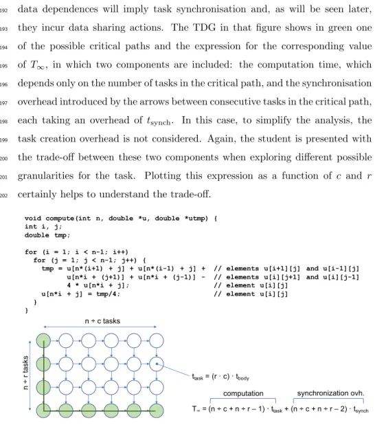
data dependences will imply task synchronisation and, as will be seen later, 192
they incur data sharing actions. The TDG in that figure shows in green one 193
of the possible critical paths and the expression for the corresponding value 194
of T∞, in which two components are included: the computation time, which
195
depends only on the number of tasks in the critical path, and the synchronisation 196
overhead introduced by the arrows between consecutive tasks in the critical path, 197
each taking an overhead of tsynch. In this case, to simplify the analysis, the
198
task creation overhead is not considered. Again, the student is presented with 199
the trade-off between these two components when exploring different possible 200
granularities for the task. Plotting this expression as a function of c and r 201
certainly helps to understand the trade-off. 202
void compute(int n, double *u, double *utmp) { int i, j;
double tmp;
for (i = 1; i < n-1; i++) for (j = 1; j < n-1; j++) {
tmp = u[n*(i+1) + j] + u[n*(i-1) + j] + // elements u[i+1][j] and u[i-1][j] u[n*i + (j+1)] + u[n*i + (j-1)] - // elements u[i][j+1] and u[i][j-1] 4 * u[n*i + j]; // element u[i][j]
u[n*i + j] = tmp/4; // element u[i][j] } } n ÷ r ta sks n ÷ c tasks ttask= (r · c) · tbody T∞= (n ÷ c + n ÷ r – 1) · ttask+ (n ÷ c + n ÷ r – 2) · tsynch
computation synchronization ovh.
Figure 4: Gauss–Seidel relaxation example and resulting TDG when each task is a block of r×cconsecutive iterations of theiandjloops, respectively. Green nodes compose one of the possible critical paths in the TDG. Computation ofT∞taking into account synchronisation overheads,tsynch.
3.3. Mapping tasks to processors
203
Once these ideas are clear, students are presented with the need to map the 204
tasks in the TDG to a particular number of processorsP in the machine. With 205
this mapping, the students can computeTp, the execution time of the tasks of 206
the program when usingP processors, and the speed-up metric, defined as the 207
quotientSp =T1/Tp. The speed-up metric, Sp, gives the relative reduction in
208
the execution time when using P processors, with respect to sequential. The 209
efficiency metric,Effp, given byEffp=Sp/P, measures the fraction of time for 210
which the processors are usefully employed. In addition, the notions of strong 211
scaling and weak scaling are introduced in a natural way during the analysis of 212
the dependence ofSp on the number of processors,P. 213
For the previous example in Figure 4, if we assume strong scaling and 214
p=n/r, thenTpwould have the same value asT∞, assuming the same
synchro-215
nisation overhead. This can be derived from the timeline shown in Figure 5. In 216
fact, only those dependences that are not internalised in the same processor (i.e. 217
that are between tasks mapped to different processors) need to be considered 218
in the computation ofTp. 219
Tp= (n ÷ c + p – 1) · ttask+ (n ÷ c + p – 2) · tsynch being p =n ÷ r and ttask= (n ÷ p) · c · tbody
S: synchronization, with overhead of tsynch
P0 P1 P2 P3 S S S S S S S S S S S S S S S S S S time
Figure 5: Timeline for the execution of tasks in the Gauss–Seidel relaxation example, assuming thatp=n/rprocessors are used.
3.4. Data sharing overhead
220
Next, the students are presented with the last source of overhead that we 221
consider: data sharing overheads. The initial simplified machine abstraction 222
used to compute the basic metrics is now leveraged in order to consider that 223
each processor has its own memory and processors are interconnected through 224
an interconnection network. Processors access local data (in their own memory) 225
using regular load/store instructions, with zero overhead. Processors can also 226
access remote data (computed by other processors and stored in their memories) 227
using remote access instructions in the form of messages. To model the overhead 228
caused by these remote accesses we consider an overhead of the formTaccess =
229
ts+m×tw, wheretsis the start-up time spent in preparing the remote access and
230
twis the time spent in transferring each element from the remote location, which
231
is multiplied by the number of elements to access,m. Additional assumptions 232
are made to simplify the model, such as that a processor Pi can only execute 233
one remote memory access at a time and only serve one remote memory access 234
from another processorPjat a time, but both can happen simultaneously. Later 235
in the course, students will see that these messages could be cache lines in a 236
shared-memory architecture or messages in a distributed-memory architecture 237
with message passing. 238
The easy-to-understandowner-computes rule can be stated at this point to 239
map data to processors. For example, for the code in Figure 4 one could say 240
that each processor will store in its local memory all those r×c elements of 241
matrixuthat are computed by the tasks assigned to it. This would result in 242
the assignment of data to processors shown in the left part of Figure 6. But 243
in order to execute each assigned task, the processor will have to access the 244
upper, lower, left and right boundary elements, which are computed by other 245
tasks (shown with different colours for one of the tasks in the same figure). 246
Some of these elements are local to processor Pi (left and right boundaries 247
in yellow and green colours, respectively) but some others are stored in the 248
memory of neighbour processorsPi−1andPi+1(upper and lower boundaries in
249
blue and orange colours, respectively). It is important to differentiate between 250
true and false data dependencies. True dependences force a task to wait for the 251
availability of data, which is what happens for the elements coloured in blue 252
(remote access happens once the producing task finishes). False dependencies 253
mean that the task has to access the data before the task that owns it starts 254
computation (elements coloured orange) because it overwrites the data due to 255
reuse. 256
Tp= (n ÷ c + p – 1) · ttask+ 1 · (ts+ n · tw) + (n ÷ c + p – 2) · (ts+ c · tw)
computation data sharing
ovh (lower) data sharing ovh (upper)
Data sharing: orange: lower boundary blue: upper boundary
time P0 P1 P2 P3 n ÷ r bl ocks n ÷ c blocks P0 P1 P2 P3
Figure 6: Data mapping (left) and execution timeline (right), including data sharing over-heads, for the mapping of tasks to processors for the Gauss–Seidel relaxation example.
Temporal diagrams, such as the one shown in the right part of Figure 6, 257
are very useful at this point to understand where remote accesses should be 258
performed (guaranteeing that when a task is ready to be executed all data that is 259
needed is available), with the possibility of reducing the number of messages due 260
to the effect ofts, which is usually much larger than tw). For example, remote 261
accesses involved in the false data dependence could be done as soon as possible, 262
at once for all tasks mapped to the same processor, before the parallel execution 263
starts, as shown in the timeline and considered in the expression ofTp. Again, 264
an analysis of the trade-off introduced by the reduction of the execution time 265
when using more processors and the data sharing overheads allows students to 266
extract interesting conclusions, having the possibilities of plotting the expression 267
for Tp that is obtained and discussing how it changes with the parameters ts 268
andtw, or even applying differentiation to see that there exists an optimum task 269
granularity. Note that, for reasons of simplicity, at this point the task creation 270
and synchronisation overheads are not explicitly considered in this analysis. 271
This unit finishes with the formulation of Amdahl’s law, allowing students 272
to understand the need for the program to have the highest possible parallel 273
fraction to parallelise. The effect of the overheads previously addressed in the 274
expression ofAmdahl’s law is also considered. 275
3.5. Methodology and support tools
276
This part of the course takes about three theory sessions (two hours each) 277
and three laboratory sessions (also two hours each) in which the students access 278
a shared-memory architecture (small cluster with nodes of 16 cores). For this 279
part of the course we also offer video material and online quizzes that cover the 280
fundamental concepts. This material is used by some professors to implement a 281
flipped–classroom methodology and offered by other professors simply as study 282
material for the students to consolidate the ideas presented in class. Finally a 283
collection of exercises is made available, some of which are solved in class in 284
order to assess the understanding of these fundamental concepts and metrics. 285
In the laboratory sessions, students take simple parallel examples written in 286
OpenMP, learning how to compile and execute them. At this point they do not 287
need to fully understand how the parallelism is expressed in OpenMP, but they 288
are able to easily capture the idea of the pragma-based parallel programming 289
approach. How to measure execution time is introduced, allowing students 290
to plot scalability as a function of the number of processors, observing how 291
easily the behaviour deviates from the ideal case. Students are presented with 292
Tareador (described in detail in [2]), a tool specifically developed to explore 293
the potential of different task decomposition strategies, visualise the TDG and 294
simulate its parallel execution. 295
Students are also presented with two tools, Extrae and Paraver, which in-296
strument and visualise the actual parallel execution and visualise some of the 297
overheads explained in class. One session is devoted to measuring those over-298
heads, observing that these overheads are non-negligible in comparison to the 299
time needed for the processor to execute an arithmetic instruction. 300
4. Task Decomposition Strategies 301
Once the fundamentals have been understood, students are faced with the 302
need to express the tasks that appear in the TDG of a sequential program, 303
which we call its task decomposition. In the proposed design, we present the 304
various task decomposition strategies for shared-memory architectures using the 305
OpenMP programming model, in particular, the OpenMP tasking model. 306
The unit starts by presenting three strategies for task decomposition: lin-307
ear, iterative and recursive. In linear decompositions, a task is simply a code 308
block or procedure invocation. In iterative decompositions, tasks are originated 309
from the body of iterative constructs, such as countable or uncountable loops. 310
Finally, in recursive decompositions, tasks are originated from recursive pro-311
cedure invocations, for example in divide-and-conquer and branch-and-bound 312
problems. 313
Three constructs from the OpenMP specification are introduced at this 314
point: parallel single,taskandtaskloop. Theparallel singleconstruct 315
simply creates a team of threads and its data context to execute tasks. In fact, 316
parallel single is the direct concatenation of two constructs in OpenMP: 317
parallel, which creates the team of threads, andsingle, which assigns to one 318
of these threads the execution of an implicit task that contains the body of 319
theparallelregion in which explicit tasks will be created using the two other 320
constructs. The single construct could be avoided, resulting in all threads 321
executing an instance of the implicit task that corresponds to the body of the 322
parallel region, replicating its execution as many times as the number of 323
threads that were created. In order to effectively perform work in parallel, the 324
programmer will have to use intrinsic functions (to know which thread is execut-325
ing the task instance) to manually decompose the work. This way of expressing 326
decompositions will be covered in a different unit, as a way to express the tasks 327
bearing in mind an explicit data decomposition strategy. 328
Thetaskconstruct is presented to students as the key component for speci-329
fying an explicit child task, whose execution will be (possibly) delegated to one 330
of the threads that are part of the team of threads. Task constructs can be 331
nested, allowing a rich set of possibilities to express parallelisation strategies. 332
Thetask pool is the main concept in the OpenMP tasking model, in which ex-333
plicit tasks are created for asynchronous deferred dynamic execution. For this 334
reason, it is important to understand how the child task’s data environment is 335
defined, partially regarding variables whose value is captured when the task is 336
created (firstprivate clause), variables that are shared with the parent task 337
(shared clause) and per-task private copies of variables (privateclause). 338
Thetaskloop construct is presented to handle the specification of explicit 339
tasks in loops, which is in fact one of the most important sources of paral-340
lelism. Thetaskloopconstruct includes two clauses to manage task granular-341
ity: grainsize(used to define the number of consecutive loop iterations that 342
constitute each task generated from the loop) and num tasks (used to define 343
the number of tasks to be generated). 344
4.1. Linear and iterative task decompositions
345
Figure 7 shows the simple vector addition example that is used in this unit 346
to illustrate the different linear and iterative task decomposition strategies and 347
how to express them using OpenMP constructs and clauses. 348
Tasking also allows the expression of iterative decompositions when the num-349
ber of iterations is unknown (uncountable), such as in problems traversing dy-350
namic data structures such as lists and trees. The list traversal in Figure 8 is one 351
of the simplest examples, showing the importance of capturing the whole scope 352
(basically the list element pointed byp) that needed by the task processing each 353
list element when executed in a deferred way (possibly) by another thread. 354
The dynamic nature of the tasking execution model does not assume any 355
static mapping of chunks of iterations (i.e. tasks) to threads, which may have 356
an important effect on data locality. These static mappings are considered later 357
in the course when covering data decomposition strategies, making use of the 358
so-called work-sharing constructs in OpenMP. We propose to present them once 359
students have been presented with the architectural support for data sharing 360
and the overheads that memory coherence may introduce when data locality is 361
not taken into account. 362
4.2. Recursive task decomposition
363
Once iterative decomposition strategies are well-understood, students are 364
faced with the necessity of expressing parallelism in recursive problems, and in 365
void main() { ....
#pragma omp parallel #pragma omp single
vector_add(a, b, c, N); ...
}
void vector_add(int *A, int *B, int *C, int n) {
#pragma omp task private(i) shared(A, B, C)
for (int i=0; i< n/2; i++) C[i] = A[i] + B[i];
#pragma omp task private(i) shared(A, B, C)
for (int i=n/2; i< n; i++) C[i] = A[i] + B[i]; }
void vector_add(int *A, int *B, int *C, int n) { for (int i=0; i< n; i++)
#pragma omp task firstprivate(i) shared(A, B, C)
C[i] = A[i] + B[i]; }
void vector_add(int *A, int *B, int *C, int n) {
#pragma omp taskloop shared(A, B, C) grainsize(BS)
for (int i=0; i< n; i++) C[i] = A[i] + B[i]; }
(a) Team of threads creation for task execution
(b) Linear task decomposition, task granularity of n/2iterations
(c) Iterative task decomposition with task, task granularity of 1 iteration
(d) Iterative task decomposition with taskloop, task granularity of BSiterations
Figure 7: Different alternatives in OpenMP to express iterative task decompositions in a vector addition example.
int main() { struct node *p; p = init_list(n); #pragma omp parallel #pragma omp single while (p != NULL) {
#pragma omp task firstprivate(p) process_work(p);
p = p->next; }
}
particular the two basic questions: “what should be a task?” and “how can I 366
control task granularities?” The first question is simply addressed by analysing a 367
recursive implementation of the vector addition example previously commented, 368
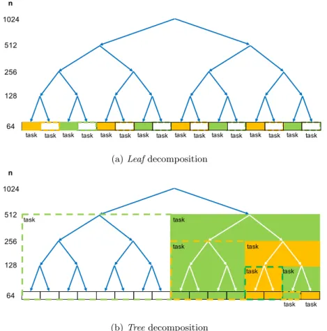
which is shown in Figure 9. Two possible decomposition strategies are presented: 369
1) theleaf strategy, in which a task corresponds to the code that is executed once 370
the recursion finishes (in the example, this is each invocation of vector add); 371
and 2) thetree strategy, in which a task corresponds to each invocation of the 372
recursive function (rec vector addin the example). Figure 10 shows the leaf 373
and tree parallel implementations of the code in Figure 9. Figure 11 shows the 374
tasks that would be generated in both cases. The main difference between the 375
two approaches is that in theleafapproach tasks are sequentially generated by 376
the thread that entered thesingleregion; however, in thetree approach tasks 377
also become task generators, so that the tasks that execute the work in the base 378
case are created in parallel. 379
4.3. Controlling task granularities
380
Once students have analysed the tasks generated in both cases, they are faced 381
with the second question, which is related to the control of task granularity. 382
With the simple observation that the task granularity depends on the depth of 383
recursion to reach the base case, students can propose different alternatives to 384
control the number of tasks generated and/or the granularity, which we call
cut-385
offcontrol mechanisms. We usually discuss three different alternatives: stopping 386
task generation (a) after a certain number of recursive calls (static control), 387
(b) when the size of the vector is too small (static control), or (c) when the 388
number of tasks generated or pending to be executed is too large (dynamic 389
control). For example, the code in Figure 12 shows how depth-based cut-off 390
control could be implemented with the leaf strategy, either using conditional 391
statements (top) or using the final and mergeable clauses available on the 392
OpenMP task construct (bottom). It is important to differentiate the base 393
case from the cut-off mechanism since they have different functionalities. 394
Other cases in which recursive task decomposition could be applied include 395
#define N 1024 #define BASE_SIZE 64
void vector_add(int *A, int *B, int *C, int n) { for (int i=0; i< n; i++) C[i] = A[i] + B[i]; }
void rec_vector_add(int *A, int *B, int *C, int n) { if (n>BASE_SIZE) { int n2 = n / 2; rec_vector_add(A, B, C, n2); rec_vector_add(A+n2, B+n2, C+n2, n-n2); } else vector_add(A, B, C, n); } void main() { rec_vector_add(a, b, c, N); }
(a) Sequential code
1024
512
256
128
64
(b) Divide-and-conquer division of the vectors A, Band C originated after recursive invocations to functionrec vector add.
Figure 9: Sequential recursive version for the vector addition example in Figure 7 and the resulting recursion tree.
branch-and-boundproblems, for example the problem of placingnnon-attacking 396
queens on a chess board or the travelling salesman problem. These together with 397
other examples based on divide-and-conquer are left to the student as problems 398
to be resolved and discussed in class. 399
4.4. Task ordering constraints
400
Once the students know the basic mechanisms available in OpenMP to ex-401
press different kinds of task decomposition strategies, together with the mecha-402
nisms to control task granularity, they are faced with the necessity of expressing 403
void main() {
#pragma omp parallel #pragma omp single
rec_vector_add(a, b, c, N); }
void rec_vector_add(int *A, int *B, int *C, int n) { if (n>BASE_SIZE) {
int n2 = n / 2;
rec_vector_add(A, B, C, n2);
rec_vector_add(A+n2, B+n2, C+n2, n-n2); } else
#pragma omp task vector_add(A, B, C, n); }
void rec_vector_add(int *A, int *B, int *C, int n) { if (n>BASE_SIZE) {
int n2 = n / 2; #pragma omp task
rec_vector_add(A, B, C, n2); #pragma omp task
rec_vector_add(A+n2, B+n2, C+n2, n-n2); } else
vector_add(A, B, C, n); }
(a) Main program
(b) Leafdecomposition
(c) Treedecomposition
Figure 10: Leaf and tree recursive task decomposition strategies applied to the vector addition example in Figure 9.
task ordering and data sharing constraints. Task ordering constraints enforce 404
the execution of (groups of) tasks in a required order while data sharing con-405
straints force data accesses to fulfil certain properties (write-after-read, exclu-406
sive, commutative, etc.). 407
Task ordering constraints can be due to control dependences (e.g. the cre-408
ation of a task depends on the outcome of one or more previous tasks) or data 409
dependences (e.g. the execution of a task cannot start until one or more previ-410
ous tasks have computed some data). These constraints can be easily imposed 411
by sequentially composing dependent tasks, by inserting (global) task barrier 412
synchronisations, which avoid the creation of tasks until the tasks that introduce 413
the control/data dependency finish, or by expressing task dependencies. 414
The two different mechanisms available in OpenMP to express task barriers 415
task task task task task task task task
task task task task task task task task
1024 512 256 128 64 n
(a)Leafdecomposition
task task task task task task task task 1024 512 256 128 64 n (b)Treedecomposition
Figure 11: Tasks generated for the leaf and tree recursive task decomposition strategies in Figure 10.
are presented to students: taskwait, which suspends the current task at a 416
certain point waiting for all child tasks to finish, andtaskgroup, which suspends 417
the current task (at the end of the structured block it defines) waiting on the 418
completion of all its child tasks and their descendent tasks. Figure 13 shows a 419
simple example that is used in class to explain these constructs. In the top-left 420
corner we have a simple TDG, showing task durations, and a trace of an ideal 421
execution of these tasks. Task barriers enforce dependences by not generating 422
tasks that depend on previously generated tasks. This causes extra delays, as 423
shown in the top-center and top-right codes and execution timelines that make 424
#define CUTOFF 3
void rec_vector_add(int *A, int *B, int *C, int n, int depth) { if (n>MIN_SIZE) {
int n2 = n / 2; if (depth < CUTOFF) {
#pragma omp task
rec_vector_add(A, B, C, n2, depth+1);
#pragma omp task
rec_vector_add(A+n2, B+n2, C+n2, n-n2, depth+1); } else { rec_vector_add(A, B, C, n2, depth+1); rec_vector_add(A+n2, B+n2, C+n2, n-n2, depth+1); } } else vector_add(A, B, C, n); } #define CUTOFF 3
void rec_vector_add(int *A, int *B, int *C, int n, int depth) { if (n>MIN_SIZE) {
int n2 = n / 2;
#pragma omp task final(depth >= CUTOFF) mergeable
rec_vector_add(A, B, C, n2, depth+1);
#pragma omp task final(depth >= CUTOFF) mergeable
rec_vector_add(A+n2, B+n2, C+n2, n-n2, depth+1); } else vector_add(A, B, C, n);
}
(a) Using conditional statements to control task generation}
(b) Using taskclauses to control task generation
Figure 12: Depth-based cut-off control for the tree recursive task decomposition strategy.
use oftaskwait. The two solutions at the bottom-left and bottom-center make 425
use of task nesting and combined use of taskgroupandtaskwaitconstructs to 426
achieve the expected behaviour, using task control mechanisms to express data 427
dependencies, but requiring “global thinking” in an unnatural way. 428
The bottom-right code and execution timeline in Figure 13 show the use 429
of task dependences in OpenMP to express the TDG in a more natural “local 430
thinking” way (having in mind only what a task requires in order to be exe-431
cuted and what it produces after being executed, independently of the task that 432
produces or uses the data). Task dependences among sibling tasks (i.e. from 433
the same parent task) are derived at runtime from the information provided 434
through directionality clauses, expressing which of the data used by the task is 435
read, written or both. 436
Task dependences are derived from the items in thein,outandinout vari-437
able lists. These lists may include array sections. Figure 14 shows another 438
example that could be used to get a better understanding of how these direc-439
foo1 foo2 foo3 foo4 foo5 5 5 5 12 4
foo1 foo2 foo3
foo4
foo5
#pragma omp task foo1()
#pragma omp task foo2()
#pragma omp taskwait #pragma omp task foo3()
#pragma omp task foo4()
#pragma omp taskwait #pragma omp task foo5() foo1 foo2 foo3 foo4 foo5 taskwait taskwait
#pragma omp task foo1()
#pragma omp task foo2()
#pragma omp task foo3()
#pragma omp taskwait #pragma omp task foo4()
#pragma omp taskwait #pragma omp task foo5() foo1 foo2 foo3 foo4 foo5 taskwait taskwait
#pragma omp task {
#pragma omp task foo1()
#pragma omp task foo2()
#pragma omp taskwait #pragma omp task foo4()
#pragma omp taskwait }
#pragma omp task foo3()
#pragma omp taskwait #pragma omp task foo5() foo1 foo2 foo3 foo4 foo5 taskwait taskwait taskwait ta sk
#pragma omp task foo3()
#pragma omp taskgroup {
#pragma omp task foo1()
#pragma omp task foo2()
}
#pragma omp task foo4()
#pragma omp taskwait #pragma omp task foo5() foo2 foo1 foo3 foo4 foo5 taskgroup taskwait
#pragma omp task depend(out:a) foo1()
#pragma omp task depend(out:b) foo2()
#pragma omp task depend(out:c) foo3()
#pragma omp task depend(in: a, b) depend(out:d) foo4()
#pragma omp task depend(in: c, d) foo5() foo1 foo2 foo3 foo4 foo5
Figure 13: Different alternatives to ensure the dependences in a simple TDG using mechanisms available in OpenMP.
tionality clauses are used. The dependences cause a wavefront execution of the 440
tasks, similar to that studied in the previous unit (Figures 4 and 5). 441
4.5. Data sharing constraints
442
Finally in this unit the student is presented with mechanisms that allow the 443
concurrent execution of tasks if exclusive access to certain variables or parts of 444
them can be guaranteed. This implies that the execution of tasks is commu-445
tative in terms of their execution order, eliminating task ordering constraints. 446
Two basic mechanisms are presented: atomic accesses, which guarantee atom-447
#pragma omp parallel private(i, j) #pragma omp single
{
for (i=1; i<n i++) { for (j=1; j<n;j++) {
#pragma omp task // firstprivate(i, j) by default
depend(in : block[i-1][j], block[i][j-1]) depend(out: block[i][j])
foo(i,j); }
} }
Figure 14: Task dependences example, simplifiedGauss–Seidelcode.
icity for load/store instruction pairs, andmutual exclusion, which ensures that 448
only one task at a time can execute the code within the critical section or access 449
certain memory locations. The three specific mechanisms in OpenMP related to 450
tasks are presented: atomic(which includes atomic updates, reads and writes), 451
critical(with and without a name) andlocks, including the intrinsic func-452
tions for acquiring and releasing locks. Understanding the differences among the 453
three mechanisms is key, and examples are used to ensure that students achieve 454
a good understanding. Code excerpts based on the use of lists, hash tables, etc., 455
are excellent examples to illustrate the differences among these mechanisms. 456
4.6. Methodology
457
This part of the course typically requires about four theory sessions (two 458
hours each) and five laboratory sessions (also two hours each). During the five 459
laboratory sessions, students receive two different assignments. Some examples 460
for these assignments are: 461
• Two-dimensionalMandelbrot Setcomputation. This is an embarrassingly 462
parallel iterative task decomposition in which students can experiment 463
with different task granularities, expressed using task and/ortaskloop 464
with different values for the grainsize. Tasks are totally independent 465
unless the result is displayed on the screen while the set is computed, in 466
which case mutual exclusion is required to plot on the screen. 467
• Sieve of Eratosthenes. The program finds (and counts) all prime numbers 468
up to a certain givenlastNumberand it is well suited for an iterative task 469
decomposition, using eithertaskor taskloopto have a better control of 470
granularity. In order to improve locality, the computation of the prime 471
numbers is done in a range betweenfrom and toand then the program 472
uses an outer loop that sieves blocks of a certain block size in order to 473
cover the full range between 1 andlastNumber. 474
• Multisort, using a divide-and-conquer recursive task decomposition strat-475
egy. The divide-and-conquer strategy recursively splits the vector to sort 476
into four parts, which are sorted with four independent invocations of 477
sort. Once these sort tasks end, two merge tasks follow, each one joining 478
the results of two sort tasks. Their results are merged again with a final 479
merge call. In this code task, task barriers (taskwait and taskgroup) 480
and task dependences are the main ingredients to effectively parallelise 481
the sequential code. 482
• Sudoku, using branch-and-bound recursive task decomposition. The code 483
is useful to show the need of data replication to enable exploratory par-484
allelisation strategies and the need to control task generation based on 485
recursion depth or the number of tasks to avoid excessive overheads. 486
For each assignment, students first useTareadorto explore possible task de-487
compositions, analyse the resulting dependences between tasks and identify the 488
variables that cause dependencies. The students try to understand the reasons 489
for the dependencies and decide how to enforce them in OpenMP. Given the 490
potential parallelism of the explored task decompositions, students start coding 491
different versions using OpenMP. As mentioned in the previous unit, Extrae
492
andParaver are used to visualise and analyse the behaviour and performance 493
of their parallelisation strategies. An analysis of overheads and strong scalabil-494
ity concludes each assignment, which also offers some optional parts to further 495
explore the possibilities of OpenMP and/or potential parallelisation strategies. 496
For this part of the course we also offer video material that covers the basic 497
task decomposition strategies and online quizzes to understand how and when 498
tasks are created and executed. As in the previous unit, this material is used 499
by some professors to implement aflipped–classroommethodology and by other 500
professors it is simply offered as study material for the students to consolidate 501
the ideas presented in class. 502
As mentioned before, students have a collection of exercises available, some 503
of which are solved in class. These exercises are an important component of the 504
course methodology to assess the understanding of different task decomposition 505
strategies and how to specify them in OpenMP via the available constructs for 506
specifying tasks, guaranteeing task ordering and sharing data. 507
5. Architecture support to shared-memory programming 508
While students practise the concepts and strategies explained in the previ-509
ous unit in the laboratory sessions, they are exposed to the basics of parallel 510
architectures, with a clear focus on understanding the support that different or-511
ganisations provide for two fundamental aspects covered in the previous units: 512
how is data shared among processors? andhow are processors able to
synchro-513
nise? Figure 15 lists the three presented architectures. 514
Memory
architecture Address space(s) Connection Model for data sharing Names
(Centralized) Shared-memory architecture Single shared address space, uniform access time Load/store instructions from processors. Snoopy-based coherence •SMP (Symmetric Multi-Processor) architecture
•UMA (Uniform Memory
Access) architecture Distributed-memory architecture Single shared address space, non-uniform access time Load/store instructions from processors. Directory-based coherence •DSM (Distributed-Shared Memory architecture •NUMA (Non-Uniform Memory Access) architecture Multiple separate address spaces Explicit messages through network interface card •Message-passing multiprocessor •Cluster Architecture •Multicomputer Processor Processor Main memory … Processor Processor Main memory … Main memory Processor Processor Main memory … Main memory
5.1. How data is shared between processors?
515
Starting from the initial cache hierarchy for single-processor architectures 516
that they already know, the students try to evolve the system to accommodate 517
more than one processor, with the objective of sharing the access to mem-518
ory. Private vs. shared cache hierarchies easily enter the discussion and the 519
cache coherence problem is presented. The two usual solutions (write-update 520
vs. write-invalidate coherence protocols) are described and their pros and cons 521
are analysed. Snoopy-based coherence mechanisms are presented first, based 522
on: 1) the fact that every cache that has a copy of a block from main memory 523
keeps its sharing status (status distributed); and 2) the existence of abroadcast
524
medium (e.g. a bus) that makes all transactions visible to all caches and defines 525
anordering. The unit then focusses on understanding the basic MSI and MESI 526
write-invalidate snooping protocols, with their states and the state transitions 527
triggered by CPU events and bus transactions. The students’ curiosity and in-528
terest easily reveal the need for more advanced protocols, such as MOESI and 529
MESIF, in order to minimise the intervention of main memory. 530
Students are questioned about the scalability of a mechanism based on a 531
broadcast medium and are helped to evolve it to a distributed solution in which 532
the sharing status of each block in memory is kept in just one location (the 533
directory). The need to physically distribute main memory across different 534
nodes while keeping cache coherence has a price: non-uniformity in terms of 535
access time to memory (NUMAarchitectures). The structure of the directory is 536
presented (the need for a sharers list in addition to the status bits) together with 537
a simplified coherence protocol and the coherence commands that are exchanged 538
between nodes (local generating the request, owner of the line in main memory 539
and remote with clean/dirty copies). 540
At this point it is important to go back to a parallel program in OpenMP 541
(such as the well known Gauss–Seidel relaxation code) and analyse how the 542
memory accesses performed by one of the tasks trigger different coherence ac-543
tions and cause changes in the state of memory/cache lines. Figure 16 shows 544
the example that is used to motivate the discussion. The example assumes 545
that 1) the blocks of the matrix are distributed in the main memories of three 546
NUMA nodes (M0−2) by rows and 2) the tasks computing the blocks in each
547
node are executed by the processor in that node (P0−2, respectively). Based
548
on that, and the dependences that order the execution of tasks, the evolution 549
of the lines shown in the figure is analysed based on the coherence commands 550
issued from the processors in each NUMA node. Students are asked to think 551
about what would happen if tasks were dynamically assigned to processors, as 552
actually happens in the OpenMP tasking model, and use this as a motivation 553
for the next unit in the subject (data decomposition strategies described in the 554
next section). 555
cache line
Access pattern:
u[i][j] = f(u[i-1][j], u[i+1][j], u[i][j-1], u[i][j+1]) Dependences:
task11can only be computed when P0 finishes with task01and the same processor (P1) finishes with task10
Questions for student discussion: Assuming uncached status for all lines at the beginning of the execution …
1. Which will be the contents of the directory for lines accessed by task01 , task10 , task12and task21when task11is ready for execution? In which caches there exist copies of those lines? (if cached)
2. And for the lines accessed by task11? 3. Repeat questions 1 and 2 above when P1is
finishing the execution of task11. P0, M0 P1, M1 P2, M2 task01 task10 task11 task21 task12
Figure 16: Example based on theGauss-Seidel computation that is used to understand the coherence traffic generated.
This is also a good point to see one of the problems that occur in cache-556
based parallel architectures: false sharingin contrast totrue sharing, and ways 557
to address it when defining shared data structures (e.g. use of padding). 558
5.2. How are processors able to synchronise?
559
Once students understand the key role of the memory system in provid-560
ing the shared-memory abstraction that OpenMP is based on, they are pre-561
sented with the need for low-level mechanisms to guarantee safety for accesses 562
to shared-memory locations (e.g. mutual exclusion and atomicity) or to signal 563
certain events (e.g. task barriers and dependences). After motivating the im-564
possibility of guaranteeing them at a higher level, the professor introduces the 565
first mechanism based on atomic (indivisible) instructions to fetch and update 566
memory on top of which other user-level synchronisation operations can be im-567
plemented: test&set (read the value at a location and replace it by the value 568
one), atomic exchange (interchange of a value in a register with a value in mem-569
ory) and fetch&op (read the value at a location and replace it with the result of 570
a simple arithmetic operation, usually add, increment, subtract or decrement). 571
Students are also presented with the other mechanism currently available based 572
on Load-linked Store-conditional instruction sequences (ll-sc), working through 573
some examples to see how to conditionally re-execute them in order to simulate 574
atomicity. 575
The basic mechanisms are used to code simple high-level synchronisation 576
patterns; after that the discussion goes back to memory coherence, analysing 577
how these synchronisation mechanisms increase coherence traffic and the interest 578
of using test-test&set or load-ll-sc whenever possible in order to avoid writing 579
to memory and invalidating other copies of the synchronisation variable. 580
This part finishes with an example in which, apparently, there is no need to 581
use any of the synchronisation mechanisms presented before to synchronise the 582
execution of tasks. The kind of example is shown on the left side of Figure 17. In 583
this code two tasks synchronise their execution through a shared variablenext; 584
the second task always goes one iteration behind the first task, doing a busy– 585
wait while loop to ensure this. This example introduces the discussion about 586
memory consistency and the relaxed consistency model used in OpenMP. The 587
same code on the right side of Figure 17 solves the problem by using#pragma 588
omp flushto explicitly force consistency. 589
5.3. Scaling through the distributed-memory paradigm
590
Finally students are questioned about the need to actually share memory 591
and presented with the third paradigm in Figure 15: multiple separate address 592
spaces. However, the simplicity of the distributed-memory paradigm in terms 593
int next = 0;
#pragma omp parallel #pragma omp single {
#pragma omp task for (int end = 0; end == 0; ) {
… next++;
#pragma omp flush(next) if (next==N) end=1; }
#pragma omp task {
int mynext = 0;
for (int end = 0; end == 0; ) { while (next <= mynext) {
#pragma omp flush(next) ; } … mynext++; if (mynext==N) end=1; } } }
Figure 17: Synchronisation through a shared variable and the use offlushto enforce consis-tency.
of hardware comes at the cost of programmability. The key point to understand 594
here is that since each processor has its own address space, a processor cannot 595
access data resident in the memory of other processors and any interaction with 596
them has to be done through the network interface card and interconnection 597
network. With the knowledge that students have about computer networks the 598
message passing paradigm flows very naturally. The basic primitives for data 599
exchange are presented, both in the form of point-to-point communication (basic 600
send and receive) and in the form of collectives (basic broadcast, scatter, gather 601
and reduction). 602
5.4. Methodology
603
This part of the course takes about three theory sessions (two hours each), 604
with no laboratory sessions. We offer to the students video material that covers 605
cache coherence for both bus and directory-based shared-memory architectures 606
and for distributed-memory architectures together with online quizzes to un-607
derstand the main concepts. As in the previous unit, this material is used by 608
some professors to implement a flipped-classroom methodology and simply of-609
fered by other professors as study material for the students to consolidate the 610
ideas presented in class. However, the video material used in this unit belong to 611
the course High Performance Computer Architecture from Georgia Tech Uni-612
versity by Profs. Milos Prvulovic and Catherine Gamboa, which is available on 613
Udacity. 614
6. Data decomposition strategies 615
Once students understand the NUMA aspect of shared-memory architec-616
tures and the lack of data sharing in distributed-memory architectures, they 617
are presented with an alternative approach to task decomposition. The new 618
approach is based on extracting parallelism from the multiplicity of data (e.g. 619
elements in vectors, rows/columns/slices in matrices, elements in a list, subtrees 620
in a tree, and so on). 621
Data decomposition is first motivated by the excessive level of implicit data 622
movement that may be introduced in NUMA architectures by a task decomposi-623
tion that is unaware of how data is accessed by tasks. The dynamic assignment 624
of tasks to processors does not favour the data locality that would be required to 625
minimise the negative effect of accessing remote data. This is motivated by the 626
conclusions drawn from the analysis of theGauss–Seidel example in Figure 16 627
and by the new synthetic example shown in Figure 18, consisting of a sequence 628
of loops in which the tasks originate from a taskloopconstruct that executes 629
chunks of consecutive iterations. Observe also the use of thenowaitclause to 630
avoid the implicit barrier at the end of eachfor construct: data dependences 631
between tasks are internalised within the execution of each implicit task. 632
#define n 100
#pragma omp parallel #pragma omp single
for (iter=0; i<num_iters; iter++) {
#pragma omp taskloop num_tasks(4)
for (int i=0; i<n; i++) b[i] = foo1(a[i]);
#pragma omp taskwait
#pragma omp taskloop num_tasks(4)
for (int i=0; i<n; i++) c[i] = foo2(b[i]);
#pragma omp taskwait
#pragma omp taskloop num_tasks(4)
for (int i=0; i<n; i++) a[i] = foo3(c[i]);
#pragma omp taskwait
}
25..49 50..74 0..24 75..99
25..49 75..99 0..24 50..74
50..74 25..49 75..99 0..24
P0 P1 P2 P3
Vectors a, b and c are distributed across the memories of the NUMA system, as follows
0..24 25..49 50..74 75..99
M0 M1 M2 M3
Possible assignment of iterations to processors (threads) in the different loops
Figure 18: Example used to illustrate the implicit data movement when task decomposition is applied. Tasks are dynamically executed by processors, as shown on the right for a possible assignment of tasks to processors. This dynamic assignment imply penalties in the access time to data accessed by the tasks.
It should be clear at this point that data locality could be easily improved if 633
the programmer takes into account the data that is accessed by each task and 634
controls the assignment of tasks to processors. The proposed parallel code in 635
the upper part in Figure 19 makes use of the implicit tasks that are generated 636
in parallel constructs in OpenMP: one implicit task per thread executing 637
the parallel region. As can be seen in the example, each implicit task queries 638
the identifier of the thread executing it (call to omp get thread numintrinsic 639
function in OpenMP) and the number of threads that participate in the parallel 640
region (call toomp get num threads intrinsic function in OpenMP). With this 641
information each implicit task decides on a range of iterations to execute, which 642
can be the same for all the loops in the sequence in order to improve data locality. 643
In this example, in addition, the use of task barriers (taskwaitin Figure 18) 644
can be avoided because data dependences between tasks are internalised within 645
the execution of each implicit task. 646
6.1. Loop vs. task-based approaches
647
This is a good point to explain the#pragma omp fordirective in OpenMP, 648
which clearly represents the “traditional” loop-based approach to teach paral-649
lelism in a large body of parallel programming courses. As shown in the lower 650
part in Figure 19 the for work-sharing construct and schedule(static [, 651
chunk]) clause in OpenMP allow the programmer to statically assign groups 652
of consecutive iterations (each group of size chunk) to consecutive threads in 653
a round-robin way; if chunkis omitted, then the compiler simply generates as 654
many groups of consecutive iterations as threads in the parallel region. 655
Thedoacross model introduced in the most recent OpenMP specification is 656
also presented as the mechanism available to define ordering constraints between 657
loop iterations. Theordered clause in theforwork-sharing construct is used 658
to indicate thedoacross execution, and thedependclauses in theordered con-659
struct are used to indicate thesourceandsinkof the dependence relationships 660
between iterations, as shown in the two examples in Figure 20. 661