Analytical and numerical analysis and simulation of heat transfer in electrical conductors and fuses

(1)

Universität der Bundeswehr München

Fakultät für Elektrotechnik und Informationstechnik

Analytical and numerical analysis and simulation

of heat transfer in electrical conductors and fuses

Audrius Ilgevicius

Vorsitzender des Promotionsausschusses: Prof. Dr.-Ing. K. Landes 1. Berichterstatter: Prof. Dr.-Ing. H.-D. Ließ 2. Berichterstatter: Prof. Habil. Dr. R. Ciegis 3. Berichterstatter: Prof. Dr.-Ing. H. Dalichau

Tag der Prüfung: 17.09.2004

Mit der Promotion erlangter akademischer Grad:

Doktor-Ingenieur

(Dr.-Ing.)

Neubiberg, den 1. November 20004

Die Dissertation wurde am 23.4.2004 bei der Universität der Bundeswehr München eingereicht.

(2)

2.3 Conservative form of the heat transfer equations………... 2.3.1 Flat cables………... 2.3.2 Round wires………... 2.3.3 Electric fuses………... 2.4 Physical material constants……... 2.5 Determination of heat transfer coefficients………... 2.5.1 Convection coefficient for the long horizontal cylinder………… 2.5.2 Convection coefficient for horizontal plate………... 2.5.3 Exact mathematical expressions of the physical constants of air.. 2.5.4 Radiation……… 2.6 Boundary conditions……….. 9 9 10 13 15 16 17 17 20 21 23 26 29 31 3 Analytical analysis of heat transfer in a steady state

3.1 Calculation of the thermo-electrical characteristics of flat cables………. 3.1.1 Vertical heat transfer with temperature- independent coefficients. 3.1.2 Vertical heat transfer with temperature-dependent coefficients… 3.1.3 Stationary solution of vertical heat transfer equation……… 3.2 Calculation of the thermo-electrical characteristics of round wires…….. 3.2.1 Radial heat transfer with temperature- independent coefficients... 3.2.2 Radial heat transfer with temperature-dependent coefficients….. 3.2.3 Stationary solution of radial heat transfer equation………... 3.3 Calculation of the thermo-electrical characteristics of fuses………. 3.3.1 Axial heat transfer with temperature- independent coefficients…. 3.3.2 Axial heat transfer with temperature-dependent coefficients…… 3.3.3 Avalanche effect in metallic conductor………. 3.3.4 Stationary solution for axial heat transfer equation………...

35 35 35 36 37 42 42 42 43 46 46 47 48 49 4. Numerical calculation of temperature behaviour in a transient state

4.1 Overview of the numerical methods used in heat transfer computation... 4.2 Fundamentals of the finite volume method (FVM)………... 4.3 Non-linear heat transfer model of electrical conductors………...

4.3.1 Approximation of heat transfer equations by FVM………... 4.3.1.1 Flat electric cable………... 4.3.1.2 Round electric wire……… 4.3.1.3 Electric fuse………... 4.3.2 Numerical implementation of boundary conditions……….. 4.3.2.1 Flat electric cable………...

51 51 54 57 58 58 61 64 66 66

(3)

ii Contents

4.3.2.2 Round electric wire……… 4.3.2.3 Electric fuse………... 4.3.3 Solution of the equation system by Newton-Raphson method…..

4.3.2.1 Flat electric cable………... 4.3.2.2 Round electric wire……… 4.3.2.3 Electric fuse………... 68 69 69 69 71 72 5. Basic considerations of the experiment and experimental setup

5.1 Basic considerations of the experiment……… 5.1.1 Direct current resistance versus temperature measurement……... 5.1.2 Direct current versus voltage measurement………... 5.2 Experimental setup………...

5.2.1 Determination of the cable conductor temperature coefficient…. 5.2.2 Determination of the cable conductor temperature………... 5.3 Measuring process and parameter acquisition………... 5.3.1 Determination of the cable conductor temperature coefficient…. 5.3.2 Determination of the cable conductor temperature………...

75 75 75 79 82 82 83 84 84 85 6. Mathematical model validation and interpolation of the numerical results

6.1 Mathematical model validation………. 6.2 Interpolation of the numerical results to reduce heat transfer equations...

89 89 97 7. Calculations of the heat transfer in a multi-wire bundle

7.1 Coordinate transformation of multi-wire bundle geometry………... 7.2 Calculation of the heat transfer in the real multi- wire bundle…………...

103 103 108 8. Summary and outlook

8.1 Summary………

8.2 Conclusions………...

8.3 Suggestions for future research……….

113 113 116 117 Appendix

A Heat transfer equations for electric conductors

A.1 Heat transfer equations for flat electric cable……… A.2 Heat transfer equations for round electric wire………. A.3 Heat transfer equations for an electric fuse element……….

119 119 121 123 B Numerical algorithm application for heat transfer simulation

B.1 Numerical heat transfer simulation and interpolation of the results…….. B.2 Calculation of thermo-electric characteristics by the polynomial

functions………

125 125 126 C Software for measurement data acquisition

C.1 Algorithm description and measurement program………

C.2 Measurement results……….. 129 129 131 Bibliography 135 Acknolegment 139

(4)

List of symbols

A surface area, m2

Af cross section area of flat cable, m2

Afu cross section area of the fuse, m2

a,b,c,d polynomial coefficients of polynomial function (in Eq. 1.1, 1.3) an,bn,cn intermediate variables in tri-diagonal matrix

b width of flat cable, m d thicknes of flat cable,m

D multi- wire bundle diameter, m E electric field strength, V/m

E0 electric field strength at reference temperature, V/m

F filling factor of multi- wire bundle f filling factor of electric wire conductor

G heat conductance in multi- wire bundle, W/mK

Gr Grashof number

g gravitational acceleration, m/s2 i spatial index in numerical calculation I electric current, A

I0 nominal electric current of electric wires or cables, A

J electric current density, A/m2

K number of time steps in numerical calculation algorithm Kd1,KT1,

KT21,KT22,

KT31

intermediate variable of heat convection equation (section 2) L characteristic length of the fuse element or cable, m

L length of the wire, m

N number of nodes in the numerical scheme

N vector size in the numerical algorithm or number of time constants

Nu Nusselt number

P electric power per unit length, W/m or perimeter, m

Pr Prandtl number

q heat flux, W/m2

qc heat flux caused by the convection, W/m2

qr heat flux caused by the radiation, W/m2

qv rate of energy generation per unit volume, W/m3

R ohmic resistance, Ω

Ra Rayleigh number

r0, r1 cylinder radius, m

r,Φ,z cylindrical coordinates

S thickness of insulation of multi-wire bundle, m

T temperature, °C

∆T temperature difference, K Tenv environment temperature, °C

Ts surface temperature of the conductor, °C

T∞ absolute temperature, K

t time, s

tg heating-up time, s

(5)

iv List of symbols

x,y,z rectangular coordinates, m

W energy rate, W

∆Wst stored energy in the solid, W

Wout energy entering the solid, W

Wint energy generated in the solid by the Joule losses, W

Wout energy rate dissipated by the solid, W

Greek Letters

α overall heat convection coefficient, W/m2K

αc heat convection coefficient, W/m2K

αr radiation coefficient

αρ,α0 linear temperature coefficient of copper resistance, 1/K

ß volumetric thermal expansion coefficient, 1/K

ßρ,ß0 square temperature coefficient of copper resistance, 1/K2

χ length constant, m

∆ Lapla ce operator

ε emissivity

? heat conductivity coefficient, W/mK

ν kinematic viscosity, m2/s

ρ density, kg/m3

ρel specific resistivity, Ωm

ρ0 specific resistivity at reference temperature 20°C, Ωm

σ Stefan-Bolzman constant

φ azimuthal angle, rad

γ specific heat capacity per volume, J/m3K

τ time constant, s

τg heating-up time constant, s

τ0 time constant at I=0, s Subscripts ave average c convection env environment el electric f flat cable fu fuse

g heating-up time notation

i spatial nodes notation in numerical algorithm r radiation, round wire

v volume

∞ free-stream conditions Superscripts

* absolute temperature - 273.15 K n time index in the numerical algorithm 4 temperature of fourth order

(6)

________________

CHAPTER

1 ________________

INTRODUCTION

Thermo-electrical investigations of electrical conductors (wires, cables, fuses) have been described in a great variety of applications and gained increasing attention by a number of research works [1,2,3,4]. The major part of these works was devoted to the analysis of heat transfer in electrical conductors for high voltage power distribution sys-tems. However, today, power supply in mobile systems like aircrafts, ships or cars have to be considered due to weight restrictions. The main difference between power lines and wires for mobile applications is the length, which does not exceeds 8 m i.e. in the cars. This causes higher current density that leads higher voltage drop.

Today, in the modern mobile vehicles electrical and electronic equipment is of great importance. Electronics is used for the applications like electromechanical drives (ser-vomotors, pumps) as well as for air conditioners and safety equipment. In the future even safety – critical systems in the cars might be replaced by so-called “x-by-wire” technology [5,6], where steering, braking, shifting and throttle is performed by electron-ics. The electronics replaces the mechanical systems due to the following reasons:

- to increase passenger comfort,

- to reduce the weight of a vehicle while increasing the inner space, - to increase safety,

- to reduce fuel consumption and costs

Since, the power consumers are distributed over the whole vehicle, the power must be delivered to the consumers by electrical wires. With increasing number of consumers, the amount of wires and the wire size rises also. Since the space in mobile systems is limited and weight is always being reduced, wire conductor sizes must be kept as small as possible. Therefore, it is necessary to investigate heat transfer in electrical conductors in order to be able to calculate optimal conductor cross-section for long lasting load. This information can be obtained from the current-temperature (= steady state) charac-teristic of each wire.

It is also important to consider current-time (= transient-state) characteristic of wires versus fuses. This information is important for the fuse design, whose current-time characteristic should match wire current-time characteristic in order to protect the wire reliable against ove rload and short-circuit currents.

The main development in the field of heat transfer computation in electric power cables was made by the work of Neher and McGrath [6] published in 1957. Later, there were a number of publications published as IEEE transactions. In 1997 based on IEEE transac-tions George J. Anders published the first book [7], which is the only devoted solely to the fundamental theory and practice of computing the maximum current a power cable

(7)

2 Chapter 1. Introduction

can carry without overheating. Almost all references to scientific articles and books of heat transfer analysis in electric cables are summarized in this book.

However, literature [7] is only devoted to the heat transfer computations for transmis-sion, distribution, and industrial applications. The problem dealing with mobile systems, is not covered by the book. The main difference between the electric cables used in in-dustrial applications and mobile systems is that the latter have generally shorter lengths and much higher operating temperature ranges.

The first attempt to develop a theory of heat transfer calculation in electric conductors for mobile applications was made by T. Schulz [8]. In his dissertation, the steady-state heat transfer equations of electric conductors have been solved analytically with some simplifications. This is sufficient to elaborate tendency. For more precise calculations, however, numerical methods should be applied.

In addition to this, there is also a need for the mathematical relationships of thermo-electrical characteristics for computer aided design program. The present available computer simulation programs for heat transfer like CableCad or Ansys [9,10] are too complex, use pure numerical methods requiring specific knowledge, and are not specia l-ized for heat transfer calculation in electric cables and fuses. On the contrary, the im-plementation of a simple mathematical model into a computer program, would allow the development of a very time-efficient cable design tool.

All this shows, that there is a requirement to investigate the heat transfer in electrical conductors and to develop efficient algorithms for the calculation of the thermo-electrical characteristics. In this study, efficient algorithms means, that all characteris-tics of conductors should be described by simple mathematical functions. One of the possible ways to solve this problem is to combine analytical and numerical analysis methods.

1.1 Objectives of current study

The aim of the present research is to analyse heat transfer of one-dimensional electric conductor models and to develop a simplified calculation methodology of thermo-electrical characteristics for computer aided electric cable design algorithms. In order to achieve this goal the following problems must be solved:

• To create one-dimensional mathematical model of electric conductors for calcu-lation of thermo-electrical characteristics of electrical cables and fuses;

• To analyze steady-state heat transfer by solving partial differential equations analytically;

• To calculate steady / transient – state characteristics using a one-dimensional numerical model;

• To verify the obtained numerical model by experimental data;

• To develop a simplified calculation methodology of electric conductor charac-teristics by fitting earlier obtained numerical results with polynomial functions.

(8)

1.2 Methodology of current research 3

1.2 Methodology of current research

This research work presents a one-dimensional (1-D) analytical and numerical model to simulate a heat transfer in flat cables, cylindrical wires and electric fuses separately.

a) _b)

Heat dissipation due to free convection and radiation to air

Heat difusion due to heat conduction to the wire

Heat dissipation due to free convection and radiation to air Heat dissipation due to free

convection and radiation to air _{convection and radiation to air}Heat dissipation due to free

c)

Copper wire PVC insulation

Fig. 1.1 Heat dissipation by free convection in electric conductor models: a) - flat cable, b) - round wire, c) - fuse

In this study both approaches i.e. analytical and numerical, are used for the analysis of heat transfer.

Analytical solutions were used to obtain steady-state temperatures for linearised con-ductor models. The linearisation was done although non- linear heat transfer models would be appreciable. The experimental data have shown that linearised model have quite a good agreement with experimental data.

Numerical model was applied for transient-state temperature calculations considering a non- linear heat transfer model.

The heat transfer in electrical systems (cables and fuses) (Figure 1.1) is obviously of two - or three -dimensional nature (2-D or 3-D). The heat transfer occurs due to the heat

(9)

4 Chapter 1. Introduction

diffusion from fuse to the wire or to the fuse holder; also the heat is dissipated from the surfaces of conductors to the ambient due to temperature differences. However, due to the complexity of the numerical model and large time scale of heat transfer processes in the cables it is not computationally efficient to use three-dimensional models to simu-late heat transfer in electrical systems. The CPU time for simulating the same physical system using two- or three -dimensional models is significantly longer than required by a simplified 1-D model. In creating a mathematical model of flat cables (Figure 1.1a) we regard heat transfer only in y – direction (see three-dimensional drawing) while side effects are negligible. Boundary conditions are symmetrical and convective-radiative. Here, convection is assumed unforced and laminar. Flat cable has insula-tion/conductor/insulation layer sequence, where the insulation is PolyVinylChloride (PVC) and the conductor is copper. Insulation layer is described by heat conductivity, specific heat capacity and heat dissipation coefficient. Conductor layer is heated with uniform volumetric heat, generated by electrical current.

In the case of cylindrical wires (Figure 1.1b), the 3-D problem is reduced to 1-D regard-ing only radial heat transfer and as infinite length of the wire. The same material proper-ties and boundary conditions apply as for flat cable.

The fuse model (1.1c) can also be considered as a cylindrical conductor, only with finite length and without insulation. The model is also reduced to a 1-D model neglecting ra-dial heat transfer, because the fuse element has very high heat conductivity. Since the fuse element has finite length, axial heat transfer is modelled with prescribed tempera-tures on the boundaries T(0,t) and T(L,t). These temperatures are known from wire tem-peratures determined earlier.

Due to the non-linear behaviour of material properties with respect to the temperature, a numerical algorithm had to be applied. A finite volume (FV) method was used to ap-proximate partial derivatives of heat transfer equation. The obtained system of non-linear algebraic equations was solved by iterative Newton-Raphson method in order to find nodal unknowns of temperatures in the conductors.

The final step of this work was the evaluation of numerical simulation results by the polynomial fitting procedure using the least square (LS) algorithm. A number of mathematical methods have been proposed [10,11,12,13,14] for the analysis of heat transfer in electrical conductors. Usually these methods are pure-analytical or numeri-cal. Analytical methods are easy to handle, physically meaningful but of limited appli-cation for complicated models (non- linear, non-homogenous) and boundary conditions. A numerical approach enables us to implement more realistic boundary conditions, which can be applied to complicated geometries. In order to understand physical mean-ing of the results received from the numerical simulation, calculation results have to be described by simple mathematical equations with as small a number of unknown vari-ables as possible. Therefore, thermo-electrical characteristics of electrical conductors are analysed by polynomial or logarithmical functions. The second reason of derivation of simplified equations is to implement these formulas into computer tool, where a very good time-efficiency can be achieved.

(10)

1.3. Scientific novelty 5

1.3 Scientific novelty

The special scientific contribution of this work is the particular way to combine analyt i-cal and numerii-cal methods to i-calculate the thermal behaviour of electrii-cal conductors. The proposed algorithm is based on the following steps:

1. Analytical derivation of the heat transfer equations.

2. Analytical solution of the obtained differential equations with mainly tem-perature independent or linear dependent physical constants.

3. Simplification of the obtained analytical solution to reduce the number of variables.

4. Numerical approximation of the heat transfer equations with non- linear tem-perature dependent phys ical constants.

5. Model validation of the numerical results by experimental data.

6. Interpolation (fitting) of the received numerical results with the simplified equations derived from the analytical solution of the heat transfer equations. 7. Evaluation of the results to receive a limited amount of independent constants (e.g. temperature) to describe the thermal-electrical characteristics with suffi-cient accuracy.

In this study, for the first time, a methodology of heat transfer analysis in electric sys-tems for mobile applications has been formulated. It is shown that it is possible to de-scribe main thermo-electrical characteristics by simplified quasi-analytical functions, which are valid for one particular conductor type.

Obtained thermo-electrical characteristics of electrical conductors are: - thermo – electrical characteristic ∆T(I) :

(

)

2 0 aI bI I I T ≤ = + ∆ (1.1) - heating-up time characteristic tg(I) :

(

)

2 0 2 2 0 0 ln I I I I I t − = > τ (1.2)

(11)

6 Chapter 1. Introduction 2 5 . 0 I d I c I − + =τ τ (1.3) Having the relationship between the conductor temperature and electrical current (Eq. 1.1), voltage drop in the conductor can be calculated as following:

- voltage drop per length characteristic E(I) :

A T T I A I E (1 ( )) 2 0 + ∆ + ∆ = = ρ ρ αρ βρ (1.4) here:

∆T conductor temperature difference against environment in K

I current in A

I0 nominal current in A

a,b,c,d constants

t heating up time in s

τ0 nominal time constant in s

τ current dependent time constant in s

τI time constant at zero current in s

E voltage drop per length in V/m

ρ specific resistance (resistivity) in Ωm

ρ0 specific resistance at reference temperature (e.g. 20°C) in Ωm

αρ linear temperature coefficient of the specific resistance in 1/K

βρ square temperature coefficient of the specific resistance in 1/K2

A conductor cross sectional area in m2

In this work an algorithm is proposed to describe thermo-electrical characteristics with the simplified equations (see above 1.1-1.4), which were obtained from analytical and numerical models. This algorithm is suited for implementation in the computer aided cable design program.

Based on the proposed algorithm to calculate thermo-electrical characteristics a com-puter program to design electrical systems in cars has been written [15].

1.4 Research approval and publications

Created methodolo gy and algorithms, which have been developed to calculate thermo-electrical characteristics of thermo-electrical cables for car applications were implemented by cable harness manufacturer Leoni Bordnetzsysteme GmbH and DaimlerChrysler AG. The basic achievements of present research have been presented at the following inter-national conferences:

(12)

1.4. Research approval and publications 7 - The 7th International Conference “Electronics’2003” in Kaunas, Lithuania, 2003; - The 8th International Conference “Mathematical Modelling and Analysis” in

Trakai, Lithuania, 2003

The content of the dissertation includes three scientific publications: the two papers are published in the journal “Mathematical Modelling and Analysis” and one publication in “Electronics and Electrical Engineering”. Both journals are edited in Lithuania by an international editorial board.

(13)

________________

CHAPTER

2

________________

PHYSICAL MODELS

OF CONDUCTORS AND

THEIR HEAT TRANSFER

EQUATIONS

2.1 Overview

Before the discussion of the theoretical model, a short “guide” will be presented at first. This “guidance” is intended to show concisely in what steps the heat transfer equations are going to be developed. It will also be discussed how these equations are solved for cable rating problems.

After a short introduction to the model geometry, heat transfer equations of different model geometries will be derived. These equations describe the temperature behaviour in electrical conductors and fuses.

As a next step, the heat convection and radiation coefficients will be determined. The heat convective coefficient is presented for cylindrical and horizontal surfaces. Because of its nonlinearity, this coefficient will have to be linearized for the later analytical analysis of the heat equation.

Following this, the main physical material parameters of the heat equation will be con-sidered. Because of its nonlinearity (e.g. heat conductivity and electrical resistance) in reality, certain simplifications have to be introduced. It will be shown that these simpli-fications can be tolerated for the thermal analysis of the electrical conductor and do not restrict the validity of the simplified thermal conductor model in the temperature range of interest.

Finally, required boundary conditions will be introduced. The y have to be linearized in order to implement them into an analytical solution of the heat equation.

With these preparations, it will be possible to investigate the thermo-electrical charac-teristics of conductors and calculate their ratings.

(14)

10 Chapte r 2. Physical models of conductors and their heat transfer equations

2.2 Geometry of physical models

On the basis of electrical conductors, three different models will be considered: flat insulated cable,

round insulated wire, and electrical fuse.

These three different types of conductors cover the main part of power supply system in many applications. In the flat cable model, the term “cable” is used because it has more than one wire. All models are one – dimensional systems, because the other dimensions in all cases vanish due to large difference between cross-sections (for a round wire or fuse) or thickness (for flat cable) and length of the conductors.

A. The flat cable model (Fig. 2.1,a) is reduced to one-dimensional heat conduction, whereby spatial derivatives with respect to x and z are neglected:

(∂_x(...)=∂_z(...)≡0).

The reduction of the model is possible because of infinite length of the cable L and much bigger width b compared to the thickness d. Due to lateral symmetry of this model, it is sufficient to analyse the upper part of the flat cable only. The model consists of three layers and can be extended depending on the flat cable structure. From “bot-tom” to “top” in the figure (2.1,a) we have:

• Polyvinylchloride (PVC) insulation

• Metallic conductors (pure copper)

• Polyvinylchloride (PVC) insulation

For the sake of simplicity, the conductors (the middle layer) are considered as a homo-geneous conductor layer.

B. In round wire model (Fig. 2.1, b) all spatial derivatives of the heat equation vanish with respect to x and ϕ:

(∂_x(...)=∂_ϕ(...) ≡0).

The heat conduction in the axial direction is neglected, because normally the length of the wire is much larger than its area, therefore, the boundary effects can be neglected. The angular dimension ϕ is also neglected due to rotational symmetry of the conductor and insulation layer. The whole model consists of two layers and can be extended to more layers, depending on the wire construction.

In this model, we have:

(15)

2.2 Geometry of physical models 11 • Polyvinylchloride (PVC) insulation y z x d b T(x,y,z,t)~T(y,t)~ Copper conductor PVC insulation y d a)

(16)

12 Chapte r 2. Physical models of conductors and their heat transfer equations 2 r_ins 2 r_c,effect r r_ins r_c Copper wire PVC insulation T(r,x,t)~T(r,t)_~

Volumetric heat generation

x T_env r in m Environment Insulation Conductor Insulation Environment T_ins _T cond Tins T_env T(r) q_v b)

(17)

2.3 Conservative form of the heat transfer equations 13

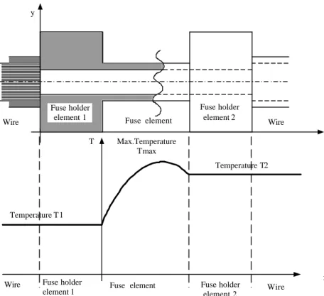
Wire

Fuse holder

element 1 _{Fuse element} _Wire Fuse holder element 2 y x Wire T Fuse holder

element 1 Fuse holder_{element 2} Wire Temperature T 1 Temperature T2 Max.Temperature Tmax x Fuse element c)

Fig. 2.1 Model geometries and heat conduction parameters: a – flat cable, b – round wire, c – electric fuse

The metallic conductor is assumed homogeneous and a perfect cylinder. In reality, the core of wire is made of a number of single conductors with small air gaps in between. If single conductors are arranged symmetrically, then the wire has a hexagonal shape. C. The electrical fuse model is one – dimensional (Fig. 2.1, c) with the heat conduction only along the x – axis. The heat conduction in y – direction is not considered because of very high heat conductivity of copper compared to the heat convection from the sur-face. The shape of the fuse model in x – direction is non-homogeneous. The whole model consists of one layer – copper, bras or any other alloy.

2.3 Conservative form of the heat transfer equations

In order to calculate heat dissipation (heat conduction, convection and radiation), the relevant heat transfer equations have to be solved. These equations define the relation-ship between the heat generated by electrical current in metallic conductor, and the tem-perature distribution within the wire or cable (conductor and insulation) and in its sur-roundings.

(18)

The analysis of heat transfer is governed by the law of conservation of energy. We will formulate this law on a energy rate basis; which means, that at any instant, there must be a balance between all power rates, as measured in Joules (= Ws). The energy conser-vation law can be written in following form:

out st

ent W W W

W + _int = + (2.1)

where:

Went is the rate of energy entering the electrical conductor. This energy may be

generated by other cables or wires located in the vicinity of other cables or by solar energy,

Wint is the rate of heat generated internally by Joule losses,

Wst is the rate of energy stored within the cable,

Wout is the rate of energy which is dissipated by conduction, convection, and

ra-diation.

The inflow and outflow terms Went and Wout are surface phenomena, and these rates are

proportional to the surface area. The thermal energy generation rate Wint is associated

with the rate of conversion of electrical energy to thermal energy and is proportional to the vo lume. The energy storage is also a volumetric phenomena, but it is simply associ-ated with an increase (Wst > 0) or decrease (Wst < 0) in the energy of cable. Under

steady-state conditions, there is, of course, no change in energy storage (Wst = 0). A

de-tailed derivation of the heat transfer equation is given in Appendix A.

From the Equation (2.1), (see also Appendix A) general form of the heat transfer equa-tion in conservative form 1in Cartesian (2.2) and cylindrical (2.2a) coordinates is ob-tained as follows [11]: t T q z T z y T y x T x v ∂ ∂ = +       ∂ ∂ ∂ ∂ +     ∂ ∂ ∂ ∂ +       ∂ ∂ ∂ ∂ _λ _λ _λ _γρ (2.2) t T q T r r T r r r x T x V ∂ ∂ = +     ∂ ∂ ∂ ∂ +       ∂ ∂ ∂ ∂ +       ∂ ∂ ∂ ∂ _γρ φ λ φ λ λ 1 1₂ (2.2a)

here: ? heat conductivity in W/mK

qV volumetric heat generation in W/m3

1

The conservative form is a form of heat conduction equation where space dependant thermal conductiv-ity or other coefficients remains conserved within different media of materials. The conservative form is given as       ∂ ∂ ∂ ∂ = ∂ ∂ x T x T T λ

γ and the nonconservative form as

x T x x T t T ∂ ∂ ∂ ∂ + ∂ ∂ = ∂ ∂ _λ λ γ 2₂

(19)

2.3 Conservative form of the heat transfer equations 15

γ specific heat capacity in W/kgK

ρ density in kg/m3

The heat equations (2.2, 2.2a) are the basis for future heat transfer analysis in electrical conductors.

2.3.1 Flat cables

The heat transfer equation (2.2) for flat cable (Fig. 2.1, a), which is derived (in Appen-dix A.1) is simplified for one-dimension as follows:

) , ( ) , ( ) , ( ) , ( ) , ( q yT t t y T T y y t y T T y y ∂ = V ∂ +     ∂ ∂ ∂ ∂ − λ γ ρ (2.3)

As mentioned in the Chapter 2.3, in this model it is considered middle symmetry (Fig.2.2). This assumption is allowed because heat convection and radiation from “top” side of the cable surface has almost the same heat dissipation rate as from the “bottom” side of the cable. It is important to emphasize, that the free convection in air situation is considered. The cable is placed horizontal in the air.

In order to simplify the model, the metallic conductor is treated as a homogeneous body across the cable width d (see Fig. 2.1,a). Here, the heat conductivity coefficient λ is space dependant, due to different material layers in the wire. The specific heat capacity term γ is a non-linear function of temperature for copper and PVC insulation. The heat generation by electrical current is expressed as qv term and is called volumetric specific

heat flux. It is a linear function of temperature in metallic conductor and vanishes in PVC insulation.

y

x

Insulation Metallic conductor

0

(20)

Here, in the equation (2.3), volumetric heat flux is expressed as:

[

1 20( 20)

]

2 20 2 2 2 2 2 − + = = ⋅ ⋅ = ⋅ ⋅ = = T A I J dl A I dl dl A I dR dV dQ qV el α ρ ρ ρ (2.4) here

ρel specific resistance of the metallic conductor given by

[

1 ₂₀( 20)

]

20 + −

= T

el ρ α

ρ in Om,

ρ20 specific resistance of the conductor at 20°C temperature

α20 copper temperature coefficient at 20°C in 1/K (α20 = 3.83. 10-3 1/K)

l length of the cable in m

J current density in A/m2

I denotes current through the wire in A

A area of metallic conductor in m2.

2.3.2 Round wires

Heat transfer in round wires is determined, in principle, by the same equation as (2.3), heat transfer in radial direction must also be considered. The general form of heat equa-tion in cylindrical coordinates is:

) , ( ) , ( ) , ( ) , ( 1 ) , ( 1 2 T r q t T T r x T T r x T T r r r T r T r r r V = ∂ ∂ +             ∂ ∂ ∂ ∂ +     ∂ ∂ ∂ ∂ +       ∂ ∂ ∂ ∂ − ρ γ λ φ λ φ λ (2.5)

Taking into account the model simplifications given earlier (see Fig. 1,b), the heat equa-tion is reduced to the one-dimensional form (see also Appendix A.2):

) , ( ) , ( ) , ( ) , ( ) , ( 1 T r q t t r T T r r t r T r T r r r ∂ = V ∂ +       ∂ ∂ ∂ ∂ − λ γ ρ (2.6)

The temperature profile in flat cables and round wires shown in Figure (2.1,a,b) under assumption, that the temperature gradient in a metallic conductor is very small due to its very high heat conductivity. In the insulation the temperature gradient is much larger. The main temperature drop, however, is between the wire surface and environment. This temperature drop is caused by convection and described by heat convection

(21)

coeffi-2.4 Physical material constants 17 cient α. Therefore, here it is very important to determine this coefficient correctly. This problem will be discussed in the section 2.5.

2.3.3 Electric fuses

The following differential equation for the heat transfer in the fuse element is given (Appendix, A.3):

[

]

) ( ) ( ) , ( ) ( ) ( ) ) , ( ( ) ( ) , ( ) ( 4 4 T q x A t t x T x A T u T t x T T T x t x T x A x V env r c = ∂ ∂ + ⋅ − + ∆ +       ∂ ∂ ∂ ∂ − ρ γ α α λ (2.7) here:

A cross section area of the fuse element in m2

αc, αr convection and radiation coefficients respectively

u circumference in m env T t x T T = − ∆ ( , ) in K

According to the model (Fig. 2.1,c), the heat transfer should be analysed only in the x direction, because of the short lengths of the fuse melting element. The mathematical model of fuse element should calculate melting temperature of the fuse. Here, radial heat conduction can be neglected due to high heat conductivity of the fuse material. In equation (2.8) the heat flux qV is derived in the same way as in equation (2.5). In

ad-dition to this, the equation is valid also for a variable cross sectional area.

2.4 Physical material constants

Heat transfer equation given in section 2.3 depends on the specific resistance, heat con-ductivity and the heat capacity of the conductor material. All three values are tempera-ture dependent, however their values are only known for certain temperatempera-tures. In order to interpolate between these given values, a linear or square function has to be used to describe the relationship. This estimation is very important in order to model the heat transfer qualitative ly.

Different calculation precision criteria are defined for the analytical approach and for the numerical approach. For the analytical approach it is necessary to have temperature independent or linear dependent constants. The numerical approach of the heat transfer model allows more precise temperature calculation in the conductors. Here, non- linear functions can be implemented for the description of the material constants.

(22)

18 Chapter 2. Physical models of conductors and their heat transfer equations The following diagrams show the exact graphical and numerical coefficients of the

spe-cific resistance, ρ, of copper, of the heat conductivity, ?, of pure copper and PVC, and of the specific heat capacity, γ, of pure copper and PVC [16]. The temperature range in the diagrams is very wide, although in this work only temperature up to 200°C has been considered. The reason of this high temperature range in the charts is to show the over-view how the coefficients behave within wide temperature range. Linear and non- linear approximation has been made using the available data.

273 373 473 573 673 773 873 973 1073 1173 1273 1373 1,50E-008 2,00E-008 2,50E-008 3,00E-008 3,50E-008 4,00E-008 4,50E-008 5,00E-008 5,50E-008 Cu Specific resistivity ρ in Ω m Absolute temperature T in K a) 273 373 473 573 673 773 873 973 1073 1173 1273 370 375 380 385 390 395 400 405 Cu Thermal conductivity λ in W/mK Absolute temperature T in K b)

(23)

2.4 Physical material constants 19 273 373 473 573 673 773 873 973 1073 1173 1273 1373 375 380 385 390 395 400 405 410 415 420 425 430 435 440 445 Cu Specific heat γ in J/kgK Absolute temperature T in K c)

Fig. 2.3 Values of: (a) specific resistance, (b) thermal conductivity and (c) specific heat capacity of pure copper

Heat conductivity and specific heat capacity values of PVC:

Temperature in °C Name of material DIN code

20 50 100

Thermal heat conductivity ? in W/Km

Polyvinylchloride PVC 0.17 0.17 0.17

Specific heat capacity γ in J/kgK

Polyvinylchloride PVC 960 1040 1530

Tab 2.1. Values of thermal conductivity and heat capacity of PVC

Approximation of the temperature dependent copper and PVC material coefficients: a) Specific resistance of copper ρ:

(

)

(

)

[

2

]

0 0 01+ T −T + T −T = ρ α_ρ β_ρ ρ

here: ρ0 specific resistance at 20°C, ρ0 = 1.75.10-8 in O m

αρ linear temperature coefficient, αρ = 4.00.10-3 in 1/K ßρ square temperature coefficient. ßρ = 6.00.10-7 in 1/K2

(24)

20 Chapter 2. Physical models of conductors and their heat transfer equations T0 – reference temperature. In this study reference temperature coincides with

environment temperature Tenv .

b) specific heat capacity of copper γ:

T

γ

α γ

γ = 0 + , 0≤T ≤200°C

here: γ0 heat capacity at 20°C reference temperature, γ0 = 381 in J/kgK

αγ approximated linear temperature coefficient of heat capacity in 1/K

αγ= 0.17 1/K

c) specific heat capacity of PVC γ:

2 0 αγT βγT

γ

γ = − + 0≤T ≤100°C

here: γ0 heat capacity at 20°C reference temperature, γ0 = 920 in J/kgK

αγ approximated linear temperature coefficient of heat capacity in 1/K

αγ= 1.3 1/K

ß_γ approximated square temperature coefficient of heat capacity in 1/K2 ßγ=0.074 1/K2

2.5 Determination of heat transfer coefficients

The heat transfer from the surface is governed by convection and radiation. This effect can be described by the corresponding convection and radiation heat transfer coeffi-cients. Both depend on the surface and environment temperatures.

Convection takes place between the boundary surface and a heat transport by a fluid (e.g. air) in motion at a different temperature. Radiation occurs by electromagnetic wave heat exchange between the surface and its surrounding environment separated by air. In this work the convective heat transfer coefficient of laminar flow has to be examined for the following two different model geometries:

- horizontal cylinder surfaces - horizontal plate surfaces

The result of this examination leads to two different heat transfer coefficients valid for round and for plate surfaces. The convection and radiation coefficient appears in the boundary conditions of the heat transfer equations for the electrical conductor models. At the lower temperatures, which are typical for electric cable applications, convection is the basic heat dissipation component (ca. 90%).

(25)

2.5 Determination of heat transfer coefficients 21 In this work, the heat transfer in electrical conductors is computed by an analytical cal-culation (of the heat conduction equations) in the steady state regime and by a numeri-cal algorithm in a transient state regime. Therefore, the convection and radiation coeffi-cients for the analytical solution has to be linearized and to be presented in an approxi-mated form in order to obtain simple but sufficiently accurate equations of the convec-tion and radiaconvec-tion coefficients. For the numerical algorithm the coefficients will be de-rived in a non- linear form since both are non- linear (temperature dependent).

2.5.1 Convection coefficient for the long horizontal cylinders

The mainly applied round geometry has been studied extensively. Many correlations exist between the different calculation methods. The literature [11] presents simple agorithms for the calculation of convective coefficients of the cylinders. This work fo l-lows the procedure proposed by [17], where many approaches of the various procedures are summarised. The equations of this procedure were validated by the experimental data in the diploma work [18]. All notations of physical constants and material proper-ties will be used from the works [17, 18].

In general, the heat dissipation by convection is defined as: )

( − _∞

= T T

q_c α_c _s (2.8)

here: Ts surface temperature of the solid in °C,

T∞=Tenv + 273.15 the absolute temperature of the fluid in K.

The convection coefficient αc can be calculated as follows:

Nu d

c

λ

α = (2.9)

here: λ heat conduction of air in W/m2K,

Nu Nusselt number

d diameter of cylinder in m.

The Nusselt number for a horizontal cylinder according to Wärmeatlas (Heat Transfer Atlas) [17] is expressed by:

2 27 8 16 9 6 1 Pr 559 . 0 1 387 . 0 752 . 0                                 + + = Ra Nu (2.10)

(26)

22 Chapter 2. Physical models of conductors and their heat transfer equations

Ra = Gr Pr (2.11)

Here: Pr Prandtl number (see Tab. 2.2) and

Gr Grashof number defined by the following equation:

2 3 ) ( v T T gd Gr= β − ∞ , (2.12)

here: g gravitational acceleration in m/s2, ß volumetric thermal expansion coefficient in 1/K,

ν kinematic viscosity in (m2/s). The ß coefficient for ideal gas with justifiable error can be considered as:

∞

=

T

1

β (2.13)

where T∞=Tenv + 273.15 - the absolute temperature of the fluid (in K)

The material constants λ, ν and Pr of air are taken from Heat Transfer Atlas [17]. These constants are dependent on the average temperature Tave:

) ( 2 1 env s ave T T T = + (2.14)

here Ts is temperature of the surface of cylinder (in °C) and Tenv – environment

tempera-ture (in °C).

With the equations (2.9) and (2.10), the convection coefficient αc is written as follows:

2 27 8 16 9 6 1 Pr 559 . 0 1 387 . 0 752 . 0                                 + + = Ra d c λ α (2.15)

Replacing in the equation (2.15) the Rayleigh number Ra, the Prandl number Pr and heat conductivity λ leads to the following form, which is only diameter d and tempera-ture difference ∆T dependant:

( )

2 6 1 1 2 1 1 1         ∆ +       = K T d K_d _T c α (2.16)

(27)

2.5 Determination of heat transfer coefficients 23 where: 12 1 =0.752λ d K , (2.17) and 6 1 2 27 8 16 9 2 1 1 Pr Pr 559 . 0 1 387 . 0                     + = v g K_T λ β (2.18)

The physical constants of air i.e. (heat conductivity λ, kinematic viscosity ν and the Prandtl number Pr) can be found in the literature [17]. For the volumetric thermal ex-pansion coefficient ß, air is considered as an ideal gas. For reference, environment tem-perature is taken.

In the table 2.2 Kd1 and KT1 values for a temperature range from 20 to 140°C are given.

Surface tempera-ture T in °C Te mper ature Tave in °C Heat conducti v-ity λ in 10-3 W/mK Kinematic viscosity ν in 10-6 m2/s Prandtl number Pr Kd1 KT1 20 20 25.67 15.35 0.7147 0.1205 1.1121 40 30 26.41 16.29 0.7133 0.1222 1.1054 60 40 27.14 17.25 0.7121 0.1239 1.0990 80 50 27.87 18.23 0.7110 0.1255 1.0928 100 60 28.58 19.24 0.7100 0.1271 1.0868 120 70 29.29 20.26 0.7091 0.1287 1.0810 140 80 30.00 21.31 0.7083 0.1302 1.0754 Average: 0.1254 1.0932

Tab 2.2. Physical constants of air for temperature from 20 to 140 °C

The averaged fo rm of the convective coefficient for temperature range from 20 to 140°C is following:

( )

2 6 1 2 1 1.0932 1 0.1254         ∆ +       = T d c α (2.19)

2.5.2 Convection coefficient for horizontal plates

For the application for flat cables the free convection of horizontal plates has been con-sidered as well. For this geometry, we have to distinguish between the convection from the top side of the plate surface and the bottom side.

(28)

24 Chapter 2. Physical models of conductors and their heat transfer equations The convection coefficient αc is calculated similar to equation (2.9):

Nu l

c

λ

α = (2.20)

here l is characteristic length, which is defined as:

P A l≡ ,

where A and P are the plate surface and perimeter, respectively.

A. The Nusselt number for the upper side of horizontal plate according to Wärmeatlas (Heat Transfer Atlas) [17] is expressed by:

a. For laminar flow:

5 1 20 11 20 11 Pr 322 . 0 1 766 . 0                         + = − Ra Nu , (2.21) here: 4 11 20 20 11 10 7 Pr 322 . 0 1 ≤ ⋅               + − Ra .

b. For turbulent flow:

3 1 20 11 20 11 Pr 322 . 0 1 15 . 0                         + = − Ra Nu (2.22) here: 4 11 20 20 11 10 7 Pr 322 . 0 1 ≥ ⋅               + − Ra .

B. The Nusselt number for the lower side of a horizontal plate has the following form (only laminar convection):

(29)

2.5 Determination of heat transfer coefficients 25 5 1 9 16 16 9 Pr 492 . 0 1 6 . 0                         + = − Ra Nu (2.23) here 10 9 16 16 9 3 10 Pr 492 . 0 1 10 <               + < − Ra

All the equations (2.1, 2.13) and Nusselt numbers given in (2.21, 2.22, 2.23) are in-serted into equation (2.20). This leads to the following form of the convection coeffi-cients: A. Upper side a. Laminar flow:

( )

15 3 8 21 1 T l K_T c  ∆      = α (2.24) here: 5 1 20 11 20 11 2 21 Pr 322 . 0 1 Pr 766 . 0                         + = − v g KT β λ (2.25) b. Turbulent flow:

( )

13 22l T K_T c = ∆ α (2.26) here: 3 1 20 11 20 11 2 22 Pr 322 . 0 1 Pr 15 . 0                         + = − v g K_T λ β (2.27)

B. Lower side (laminar flow only):

( )

15 3 8 31 1 T l K_T c  ∆      = α (2.28) here:

(30)

26 Chapter 2. Physical models of conductors and their heat transfer equations 5 1 9 16 16 9 2 31 Pr 322 . 0 1 Pr 6 . 0                         + = − v g KT β λ (2.29)

2.5.3 Exact mathematical expressions of the physical constants of air

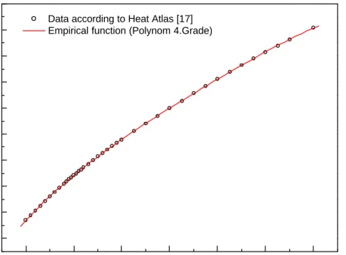
The physical constants of air depend very much on temperature. These functions are of higher polynomial order, which were obtained by fitting of the given results in the Wärmeatlas [17]. With these functions, a very high accuracy of conve ction coefficient can be achieved and the function can easily be implemented into the computer program. Here, the wide temperature range is used in order to expand the validity range of tem-perature dependent constants in the computer program.

A. Heat conductivity in air λ (Tave):

Temperature range for the fitting procedure: −200 °C≤T_ave ≤1000°C Obtained polynomial function by fitting:

4 14 3 11 2 8 5 10 99059 . 1 10 36064 . 4 10 3282 . 4 10 61617 . 7 02416 . 0 ) ( ave ave ave ave ave T T T T T − − − − ₋ _⋅ ₊ _⋅ ₋ _⋅ ⋅ + = λ (2.30)

(31)

2.5 Determination of heat transfer coefficients 27 -200 0 200 400 600 800 1000 0 10 20 30 40 50 60 70 80 90

Data according to Heat Atlas [17] Empirical function (Polynom 4.Grade)

Heat conductivity of air

λ in 10 -3 Wm -1 K -1 Temperature T_ave in °C

Fig. 2.4 Heat conductivity of air as a function of temperature at constant pressure P = 105 Pa

B. Kinematic viscosity ν(Tave):

Temperature range for the fitting procedure: −200°C ≤T_ave ≤1000°C Obtained polynomial function by fitting:

4 17 3 14 2 10 8 5 ₈_.₈₂₄₀₂ ₁₀ ₁_.₁₄₁₇₁ ₁₀ ₄_.₆₄₆₃ ₁₀ ₁_.₆₄₈₈₂ ₁₀ 10 35391 . 1 ) ( ave ave ave ave ave T T T T T − − − − − ₊ _⋅ ₊ _⋅ ₋ _⋅ ₊ _⋅ ⋅ = ν (2.31)

(32)

28 Chapter 2. Physical models of conductors and their heat transfer equations -200 0 200 400 600 800 1000 0 500 1000 1500

2000 Data according to Heat Atlas [17]

Empirical function (Polynom 4. Grade)

Kinematic viscosity ν in 10 -7 m 2 s -1 Temperature T ave in °C

Fig. 2.5 Kinematic viscosity of air as a function of temperature at cons tant pressure P = 105 Pa

C. Prandtl number Pr(Tave)

Temperature range for the fitting procedure: −125°C≤Tave ≤650°C Obtained polynomial function by fitting:

4 13 3 10 2 7 4 10 32316 . 4 10 11289 . 9 10 91108 . 6 10 6855 . 1 71779 . 0 ) Pr( ave ave ave ave ave T T T T T − − − − ₊ _⋅ ₋ _⋅ ₊ _⋅ ⋅ − = (2.32)

(33)

2.5 Determination of heat transfer coefficients 29 -200 0 200 400 600 800 1000 0.68 0.70 0.72 0.74 0.76 0.78 0.80 0.82 0.84 0.86 0.88 650°C -120°C

Empirical funktion (Polynom 4.Grade) for Temperature range -120°C < T

ave < 650°C

Data according to Heat Atlas [17]

Prandtl-number Pr

Temperature T_ave in °C

Fig. 2.6 Prandtl-number of air as a function of temperature at constant pressure P = 105 Pa

2.5.4 Radiation

In order to describe heat transfer by the thermal radiation in electrical conductors, the exchange of radiation energy between the insulated conductor surface and the infinitely large environment is considered.

It may occur not only from solid surfaces but also from liquids and gases [11]. The en-ergy of the radiation is transported by electromagnetic waves (or alternatively, photons). While the transfer of energy by conduction or convection requires the presence of a ma-terial medium, radiation does not. In fact, radiation transfer occurs most efficiently in a vacuum. The complete electromagnetic spectrum is shown in Figure 2.7. The short wavelength gamma rays, X rays and ultraviolet (UV) radiation are primarily of interest to the high energy physicist and nuclear engineer, while the long wavelength micro-waves and radio micro-waves are of concern to the electrical engineers. It is the intermediate portion of the spectrum, which extends from approximately 0.1 to 100 µm. It includes a part of the UV and all of the visible infrared (IR), that is called thermal radiation and belongs to heat transfer.

(34)

30 Chapter 2. Physical models of conductors and th eir heat transfer equations 10-5 ₁₀-4 ₁₀-3 ₁₀-2 ₁₀-1 ₁ ₁₀ ₁₀2 ₁₀3 Gamma rays X rays Thermal radiation 0.4 0.7 Microwave Infrared Ultraviolet

Voilet Blue Green _Yellow Red

Visible

λ, µm

Fig. 2.7 Spectrum of electromagnetic radiation

The maximum flux (W/m2) at which radiation may be emitted from a surface is given by the Stefan-Boltzmann law:

4

s

r T

q =σ (2.33)

where TS is the absolute temperature (K) of the surface and σ is the Stefan-Boltzmann

constant (σ =5.67⋅10−8W/m2K4). Such a surface is called an ideal radiator or black body. The heat flux emitted by a real surface is less than that of the ideal radiator and is given by

4

s

r T

q =εσ (2.34)

where ε is a radiative property of the surface called the emissivity. This property ind i-cates how efficiently the surface emits compared to an ideal radiator.

The rate of heat exchange between the cable surface and its surroundings, expressed per unit area of the surface, is:

(

4 4

)

env s

r T T

q =εσ − (2.35)

In order make it compatible with heat convection, it is convenient to express the radia-tion heat exchange in the form:

(

s env

)

r

r T T

(35)

2.6 Boundary conditions 31 where from Equation (2.35) the radiation heat transfer coefficient αris:

(

)

(

2 2

)

env s env s r ≡εσ T +T T +T α (2.37) Here we have modelled the radiation in the same way as convection. In this sense we have linearised the radiation rate equation, making the heat rate proportional to a tem-perature difference rather than to the difference between two temtem-peratures to the fourth power. Note, however, that αr depends strongly on temperature, while the temperature dependence of the convection heat transfer coefficient αc is generally weak.

Since the free convection and radiation transfer occurs simultaneously, the convection and radiation has to be added. Then the total rate of heat transfer from the surface is as follows: ) ( ) ( _s _env _s4 _env4 c r c q T T T T q q = + =α − +εσ − (2.38)

The total heat transfer by convection and radiation expressed as the heat transfer coeffi-cient α is:

(

)

(

2 2

)

env s env s c r c+ = + T +T T +T =α α α εσ α (2.39)

2.6 Boundary conditions

In order to have a unique solution of the PDE (partial differential equation), boundary and initial conditions have to be specified as shown below. In case of differential equa-tions for the electrical fuse, prescribed boundary conditions are used. PDE’s of flat and round electrical cables will have symmetry and non-linear convective-radiative bound-ary cond itions.

1. Flat electrical cable - initial condition ) ( ) 0 , (y T y T = _env (2.40)

(36)

32 Chapter 2. Physical models of conductors and their heat transfer equations - boundary conditions

(

)(

)

(

)

       − + − ∆ = ∂ ∂ − = ∂ ∂ = → . , , 0 ) , ( lim 4 4 0 env env y y y T T T T T l y T y t y T N εσ α λ λ (2.41)

2. Round electrical wire - initial condition ) ( ) 0 , (r T r T = _env (2.42) - boundary conditions

(

)(

)

(

)

      − + − ∆ = ∂ ∂ − = ∂ ∂ = → . , , 0 ) , ( lim 4 4 0 env env r r r T T T T T d r T r t r T r N εσ α λ λ (2.43) 3. Electrical fuse - initial condition ) ( ) 0 , (x T x T = env (2.44) - boundary conditions    = = ) ( ) , ( ) ( ) , 0 ( 2 1 t T t x T t T t T (2.45)

The boundary and initial conditions in equations (2.40-2.45) are generally valid and im-plemented into the numerical algorithm of heat transfer calculations.

In the analytical analysis of heat transfer (Chapter 3), some additional boundary cond i-tions will be used to solve the PDE of flat cables and round wires. Here we have to cal-culate with the constant heat transfer coefficient and do not take into account the non-linear phenomena of radiation.

(37)

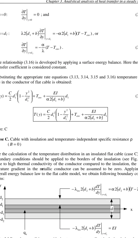
2.6 Boundary conditions 33        − − = + − = = = ) ( , ) ( 2 1 0 env ins y y ins y y T T dy dT b d EI dy dT λ α λ (2.46)

In case of cylindrical wire:

       − − = − = = = ) ( , 2 1 0 0 env ins r r ins r r T T dr dT r EI dr dT λ α λ π (2.47)

(38)

________________

CHAPTER

3

________________

ANALYTICAL ANALYSIS

OF HEAT TRANSFER

IN A STEADY STATE

In the preceding Chapter 2, a definition of heat transfer equations for the study of ana-lytical and numerical heat transfer computation was given. The objective of those equa-tions is to determine the temperature field in different kinds of electrical conductors where heat conduction, convection/radiation and energy generation takes place. Differ-ent boundary conditions were also given for the solutions of those equations.

The aim of the present chapter is to obtain exact analytical solutions in a steady-state regime. Because of the linearization of differential equations, some difference between numerical and analytical results will occur, but these mismatches can be accepted in many situations. It is always convenient to have a simple analytical solution if a steady state is required.

The following assumptions are made to simplify the partial differential equations: a) steady-state conditions,

b) one-dimensional conduction,

c) constant or linear material properties, d) uniform volumetric heat generation, e) constant heat transfer coefficient.