Arkadiusz Szymczak
∗, Maciej Paszyński
∗, David Pardo
∗∗GRAPH GRAMMAR BASED PETRI NET
CONTROLLED DIRECT SOLVER ALGORITHM
In this paper we present the Petri net setting the optimal order of elimination for direct solver working withhprefined finite finite element meshes. The computational mesh is rep-resented by a graph, with graph vertices corresponding to finite element nodes. The direct solver algorithm is expressed as a sequence of graph grammar productions, attributing the graph vertices. The Petri net dictates the order of graph grammar productions, representing the execution of the solver algorithm over a graph representation of computational mesh. The presentation is concluded with numerical experiments performed for a model L-shape domain.
Keywords: Petri nets, graph grammar, direct solver
ALGORYTM SOLVERA DOKŁADNEGO
STEROWANY SIECIĄ PETRIEGO
WYKORZYSTUJĄCY GRAMATYKI GRAFOWE
W artykule przedstawiona została sieć Petriego sterująca kolejnością wykonania produkcji gramatyki grafowej reprezentującej wykonanie algorytmu solvera dokładnego na h adap-towanej siatce metody elementów skończonych. Siatka obliczeniowa przedstawiona została w postaci grafu, którego wierzchołki odpowiadają węzłom elementów skończonych. Algo-rytm solvera dokładnego wyrażony jest w postaci sekwencji produkcji gramatyki grafowej, atrybutujących wierzchołki grafu. Sieć Petriego określa kolejność wykonania produkcji gra-matyki grafowej, reprezentujących wykonanie algorytmu solvera na grafowej reprezentacji siatki obliczeniowej. Artykuł podsumowuje eksperyment numeryczny dotyczący wykonanie algorytmu solvera na problemie modelowym w kształcie litery L.
Słowa kluczowe: sieci Petriego, gramatyki grafowe, solvery dokładne
∗Department of Computer Science, AGH University of Science and Technology, al. Mickie-wicza 30, 30-059, Kraków, Poland,[email protected]
∗∗Departamento de Matem´atica Aplicada, Estad´ıstica e Investigación Operativa, UPV/EHU, Campus de Leioa, Vizcaya, and IKERBASQUE (Basque Foundation for Sciences), Bilbao, Spain
by graph grammar for two dimensional rectangular [3], two dimensional triangular [4], as well as three dimensional tetrahedral elements [5]. The order of execution of graph grammar productions can be expressed by control diagram [11] or, alternatively, by Petri nets [6, 7]. The Petri nets model allows to analyze the correctness as well as potential for deadlock or starvation of the considered algorithms.
In this paper we focus on modeling the solver algorithm by using graph grammar based Petri nets. To illustrate it, we utilize the two dimensional L-shape domain model problem [1, 2], solved by using hrefined two dimensional rectangular finite element mesh with uniform polynomial order of approximation p.
The frontal solver is a sophisticated implementation of a Gaussian elimination algorithm suitable for sparse matrices [9]. It browses finite elements one by one, ag-gregating the element local matrices into a single frontal matrix, and eliminating fully assembled degrees of freedom. The multi-frontal solver [10] is a generalization of a frontal solver algorithm by using multiple frontal matrices. It can be efficiently used whenever the elimination tree is created, with frontal matrices assigned to the elimination tree nodes. During the execution of a multi-frontal solver algorithm, the elimination tree is processed, and frontal matrices coming from son nodes are merged at parent nodes into a new single frontal matrix. The process is recursively repeated until we reach the root of the elimination tree.
The process of mesh generation and h refinement expressed in terms of graph grammar results in a graph representation of the computational mesh. The solver algorithm will be expressed in terms of graph grammar productions controlled by the Petri nets.
2. L-shape domain model problem
In this section we introduce the L-shape domain model problem [1, 2]. The problem consists in solving Laplace equation
∆u= 0 in Ω (1)
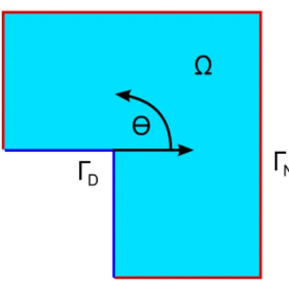
over the L-shape domain Ω presented in Figure 1. The solutionu: R2⊃Ω3u7→R is a temperature distribution inside the L-shape domain.
The zero Dirichlet boundary condition
Fig. 1.The L-shape domain
is assumed on the internal part of the boundary ΓD. The Neumann boundary
condi-tion
∂u
∂n =g on ΓN (3)
is assumed on the external part of the boundary ΓN. The exact solution with the
origin point located atO (Fig. 1) is given by: g(r, θ) =r23sin2 3 θ+π 2 . (4)
The so-calledstrong form of the partial differential equation (PDE) (1-3) is
trans-formed intoweak (variational) form of PDE
b(u, v) =l(v) ∀v∈V, (5) b(u, v) =Z Ω∇ u∇vdx, (6) l(v) =Z ΓN gvdS (7)
by considering L2(Ω) scalar products of (1) with test functions from the functional spaceV V ={v∈L2(Ω) : Z Ω kvk 2+ k∇vk2dx <∞:tr(v) = 0 on ΓD}, (8)
integrating by parts, and including boundary condition (3).
The Finite Element Method consists in constructing a subspace Vhp ⊂V with
finite dimensional basis{ei
hp}i=1,...,Nhp. The subspaceVhpis constructed by
partition-ing the domain Ω into finite number of elements, and definpartition-ing basis functions at finite element vertices, over edges, and interiors. The exemplary partition of the L-shape domain into three rectangular finite elements is presented in Figure 2.
Fig. 2.Partition of the L-shape domain into three finite elements
Elements of the basis ei
hp restricted to a particular element are called shape functions. We define the first order shape functions (pyramids) at element vertices,
second order shape functions (edge-bubbles) over element edges, and second order shape functions over elements interiors, presented in Figure 3.
Fig. 3.Examples of vertex, edge and interior shape-functions
The exact solutionuof the weak formulation (5)–(7) is approximated in subspace Vhp as a linear combination of the basis functions
u≈uhp= 21 X i=1 uihpeihp (9) The coefficientsui
hp are calleddegrees of freedom (d.o.f.). The degrees of freedom can
be obtained by solving the following system of equations 21 X i=1 uihpb eihp, e j hp =lejhp j= 1, ...,21 (10) beihp, e j hp = Z Ω∇e i hp∇e j hpdx (11)
lejhp
=Z
ΓN
gejhpdS (12)
obtained by substituting (9) into (5) and considering{ejhp},j= 1, ...,21 test functions.
3. Expressing the solver algorithm by graph grammar
production controled by Petri nets
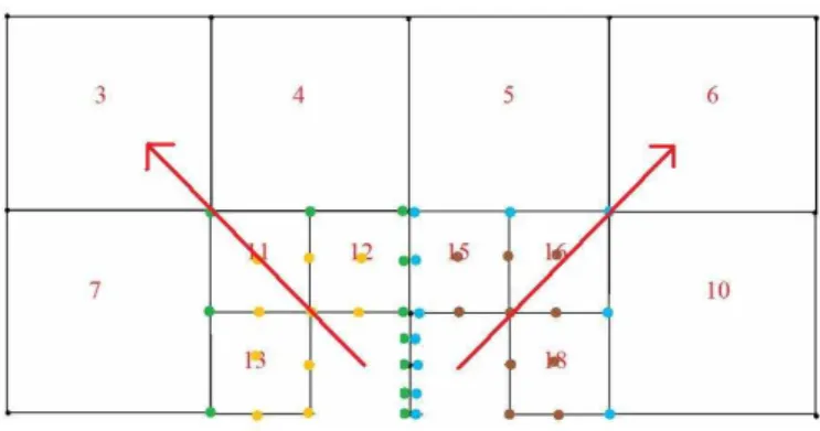
The direct solver is used to solve the system of linear equation (10)–(12). Following [12, 13] the general idea of the solver is summarized in Figure 4. The solver discussed in [12, 13] creates two frontal matrices for each refinement tree. The solver browses elements from refinement tree from the bottom to the top, aggregates d.o.f. from elements nodes to frontal matrices, and eliminates d.o.f. related to fully assembled nodes. The situation presented in Figure 4 corresponds to the case where two leaf elements have been already aggregated to two frontal matrices, and their interior nodes have been eliminated. Now, the solver have aggregated three new elements to each frontal matrix, located one level up at the refinement tree. The fully assembled nodes that can be eliminated now are denoted by yellow color for the first frontal matrix, and by brown color for the second frontal matrix. The not fully assembled nodes are denoted by green and blue colors. The disadvantage of this method is the fact that the number of not fully assembled d.o.f. on the border of two refined elements is constantly growing while we go up the refinement tree. This results in constant increase of the size of each of the two frontal matrices, which in turns slows down the solver algorithm. These nodes will be eliminated at the very end, when we reach the roots of the two refinement trees, and the two frontal matrices will be merged. The alternative strategy proposed in this paper is to merge frontal matrices coming from neighboring refinement trees before going up the refinement tree. The
idea is illustrated in Figure 5. This simple trick results in constant size of the frontal matrix.
We focus on the computational mesh presented in Figure 6 for the L-shape do-main problem, h refined in the direction of the central singularity. The graph rep-resentation of 1/3 of such a mesh, corresponding to any of the three initial mesh elements, four timeshrefined, is presented in Figure 7. The graph can be obtained by executing a sequence of graph grammar productions described in [11]. The full graph for the three refined elements is too large to be presented in a figure here.
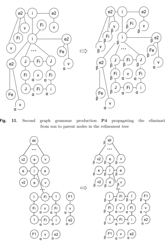
There are five graph grammar productions responsible for execution of the direct solver algorithm, presented in Figures 8–12.
The productions attribute by α or β symbols the graph vertices representing element interiors, edges and vertices. The symbols represent the aggregation into a frontal matrix, and the elimination of the node, for different levels of the refinement tree.
Fig. 4. Following the refinement trees results in increase of the size of the frontal matrix. Green and blue colors denote the growing number of border nodes
Fig. 5.Merging the frontal matrices and elimination of the border d.o.f. results in the constant size of the frontal matrix. Green color denotes the constant number of border nodes
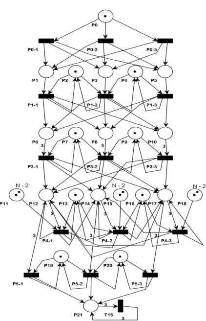
Figure 13 presents the Petri net modeling the elimination process of the solver algorithm. The sequence of elimination is represented by attributing the adaptation tree.
The analyzed example is a L-shaped mesh comprising three initial elements. The elements are numbered from 1 to 3 such that the middle element has number 2.N is the number of adaptation levels and, in the analyzed example,N = 4. The transitions are named after graph grammar productions they represent. The numbers after dash in the transition names designate the number of the mesh element being attributed by given transition. The elimination process is performed in different stages: first, production P0 is executed, then all P1 productions are executed, second all P3 and so on. Productions attributing adjacent mesh elements (1 and 2 or 2 and 3) modify vertices representing the common edge between the elements – therefore such production pairs cannot be executed in parallel.
Fig. 6.Left panel: 20 timeshrefined mesh for the L-shape domain problem.Right panel:
Amplification by a factor of 10 towards the central singularity
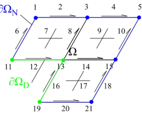
Fig. 7. Graph representation of 1/3 of the mesh for the L-shape domain problem, after fourhrefinements
Fig. 8.Graph grammar productionPO attributing the corner vertex
Fig. 9.Graph grammar productionP1 attributing the leaf of the refinement tree
Fig. 10. First graph grammar production P3 propagating the elimination from son
Fig. 11. Second graph grammar production P4 propagating the elimination
from son to parent nodes in the refinement tree
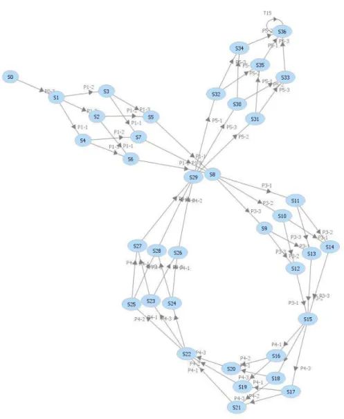
Figure 14 presents the reachability graph generated with Platform Independent Petri Net Editor for the Petri net presented in Figure 13 and initial marking of (1,0,1,0,1,0,0,1,0,1,0,2,0,1,0,2,1,0,2,1,1,0) (a number at given position indi-cates the number of tokens in the corresponding place). This graph has been ana-lyzed for deadlock occurrence with the same software. To enable such analysis, one additional place (P21) and transition (T15) have been artificially added to the Petri net. Thanks to this addition, the net becomes live if a dead state cannot be reached elsewhere. The analysis proved that the Petri net is live indeed so there is no risk of deadlock in so defined elimination algorithm.
4. Numerical experiments
The solver algorithm has been executed for the L-shape domain problem, over a computational mesh that has been 20 times h refined in the direction of central singularity, see Figure 6. The polynomial order approximation has been uniformly set to p over the entire mesh. Thus, the resulting number of d.o.f. is (p−1)2 in element interiors,p−1 over element edges and 1 at element vertices. The sequence of experiments has been performed forp= 2,3,4, ...,8. The execution time of the solver algorithm has been measured, compare Figure 15 with the following parts:
•partial forward elimination part, responsible for merging element nodes (deciding
which nodes are fully assembled and can be eliminated) as well as for merging of suitable frontal matrices,
•dgemm part denoting the time spent by matrix-matrix computations within the
LAPACK calls,
•total denoting the sum of the two above parts,
•frontal solver denoting the total execution time of the algorithm traveling the
refinement trees separately, one by one, suffering from the increase of the size of the frontal matrices,
•integration corresponding to the total integration time over all finite elements.
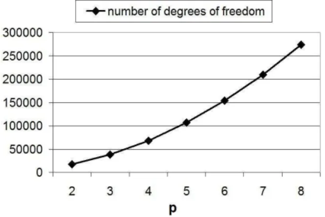
Additionally, Figure 16 presents the number of d.o.f. over the computational mesh from Figure 6, for different polynomial orders of approximationp= 2,3,4, ...,8. In other words, we compare our algorithm with the frontal solver and the integration algorithms. The reason why we do not compare the algorithm with the multi-frontal algorithm, e.g. MUMPS [14] is because for the L-shape domain problem with a single singularity there are between one and two fronts just following the refinement tree from the bottom to the top of the refinement trees.
Fig. 13. Petri net setting the order of execution of graph grammar productions expressing the solver algorithm
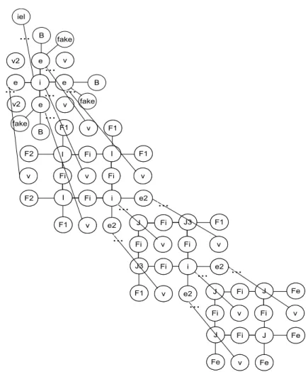
Fig. 14. The linear structure of the reachability graph for the Petri net expressing the solver algorithm. The length of the reachability graph depends on the number of executed
Fig. 15. Execution times for different parts of the Petri nets based solver as well as for the frontal solver and for the integration algorithms
Fig. 16.Sizes of the computational meshes for different polynomial orders of approximation
5. Conclusions
The proposed algorithm scales very well. Actually, the partial forward elimination
execution time does not depend onp, since the structure of nodes within the mesh does not change when we perform global prefinement. The execution time is increasing slightly for the LAPACK dgemm part, but the increase is not so rapid as for the
frontal solver algorithm suffering from the constant increase of the size of the frontal matrix. However, the frontal solver is faster for small p. This is because the frontal solver algorithm utilized in this example does not work on the level of nodes, rather it works directly on frontal matrix, and the algorithm is free from the overhead resulting
Acknowledgements
The work has been supported by Polish MNiSW grant no. NN 519 447739. The work of the third author was partially funded by the Spanish Ministry of Science and Inno-vation under project MTM2010-16511.
References
[1] Babuśka I., Guo B.: The hp-version of the finite element method. Part I: The basic approximation results. Comput. Mech., vol. 1, 1986, pp. 21–41.
[2] Babuśka I., Guo B.:Thehp-version of the finite element method. Part II: General results and applications. Comput. Mech., vol. 1, 1986, pp. 203–220.
[3] Paszyński M., Paszyńska A.: Graph transformations for modeling parallel hp-adaptive FEM computations. Lecture Notes in Computer Science, vol. 4967, 2007,
pp. 1313–1322.
[4] Paszyńska A., Paszyński M., Grabska E.: Graph Transformations for Modeling hp-Adaptive Finite Element Method with Triangular Elements. Lecture Notes in
Computer Science, vol. 5103, 2008, pp. 604–614.
[5] Paszyński M., Pardo D., Paszyńska A.:Parallel multi-frontal solver for p adap-tive finite element modeling of multi-physics computational problems. Journal of
Computational Science, vol. 1, 2010.
[6] Szymczak A., Paszyński M.:Graph grammar based Petri nets model of concurren-cy for self-adaptive hp-Finite Element Method with rectangular elements. Proc.
of Conference Parallel Processing and Applied Mathematics, 2009.
[7] Szymczak A., Paszyński M.:Graph grammar based Petri nets model of concurren-cy for self-adaptive hp-Finite Element Method with triangular elements. Lecture
Notes in Computer Science, vol. 5545, 2009, pp. 845–854.
[8] Demkowicz L.: Computing with hp-Adaptive Finite Elements, Vol. I. One and Two Dimensional Elliptic and Maxwell Problems. Chapman & Hall / CRC
Ap-plied Mathematics & Nonlinear Science, 2007.
[9] Irons B.: A frontal solution program for finite-element analysis. International
Journal of Numerical Methods in Engineering, vol. 2, 1970, pp. 5–32.
[10] Duff I.S., Reid J.K.:The multifrontal solution of indefinite sparse symmetric lin-ear systems. ACM Transactions on Mathematical Software, vol. 9, 1983, pp. 302–
[11] Paszyński M.:On the Parallelization of Self Adaptive hp-Finite Element Method. Part I. Composite Programmable Graph Grammar Model Fundamenta
Informa-ticae, vol. 94, 2009, pp. 411–434.
[12] Paszyński M., Schaefer R.: Graph grammar driven parallel partial differential equation solver. Proc. of Concurrency & Computations, Practise & Experience,
2010.
[13] Paszyński M., Pardo D., Torres-Verdin C., Demkowicz L., Calo V.: A Parallel Direct Solver for the Self-Adaptive hp Finite Element Method. Journal of Parallel
and Distributed Computing, vol. 70, 2010, pp. 255–276.
[14] A MUltifrontal Massively Parallel sparse direct Solver.http://www.enseeiht. fr/lima/apo/MUMPS/.