Bayesian Analysis of Spatial Point Patterns

(1)

Bayesian Analysis of Spatial Point Patterns

by

Thomas J. Leininger

Department of Statistical Science Duke University

Date:

Approved:

Alan E. Gelfand, Supervisor

Robert L. Wolpert

Merlise A. Clyde

James S. Clark

Dissertation submitted in partial fulfillment of the requirements for the degree of Doctor of Philosophy in the Department of Statistical Science

in the Graduate School of Duke University 2014

(2)

Abstract

Bayesian Analysis of Spatial Point Patterns

by

Thomas J. Leininger

Department of Statistical Science Duke University

Date:

Approved:

Alan E. Gelfand, Supervisor

Robert L. Wolpert

Merlise A. Clyde

James S. Clark

An abstract of a dissertation submitted in partial fulfillment of the requirements for the degree of Doctor of Philosophy in the Department of Statistical Science

in the Graduate School of Duke University 2014

(3)

(4)

Abstract

We explore the posterior inference available for Bayesian spatial point process mod-els. In the literature, discussion of such models is usually focused on model fitting and rejecting complete spatial randomness, with model diagnostics and posterior in-ference often left as an afterthought. Posterior predictive point patterns are shown to be useful in performing model diagnostics and model selection, as well as providing a wide array of posterior model summaries. We prescribe Bayesian residuals and methods for cross-validation and model selection for Poisson processes, log-Gaussian Cox processes, Gibbs processes, and cluster processes. These novel approaches are demonstrated using existing datasets and simulation studies.

(5)

(6)

List of Tables

3.1 Coverage of the various innovations and residuals in the Monte Carlo

test targeting a 90% coverage rate. . . 65

3.2 Coverage of the 90% credible intervals for the innovations and residuals

in the Monte Carlo test for thinning levels p = 0.5,0.8 and q = 0.05.

The coverage on the training dataset is given before the forward slash

and the coverage on the test dataset is given after the forward slash. . 72

4.1 RPS scores for the HPP and Strauss models on the Swedish pines

data. The coverage of the 90% intervals are given in parentheses. . . 98

4.2 The posterior p-values for the posterior predictive variance metrics

using random boxes of varying sizeq|D|. . . 102

4.3 Number of times (out of 10) having best RPS score on a simulated

dataset under each type of data-generating process, with _E[n]≈100. 110

4.4 Number of times (out of 10) having best RPS score on a simulated

(10)

List of Figures

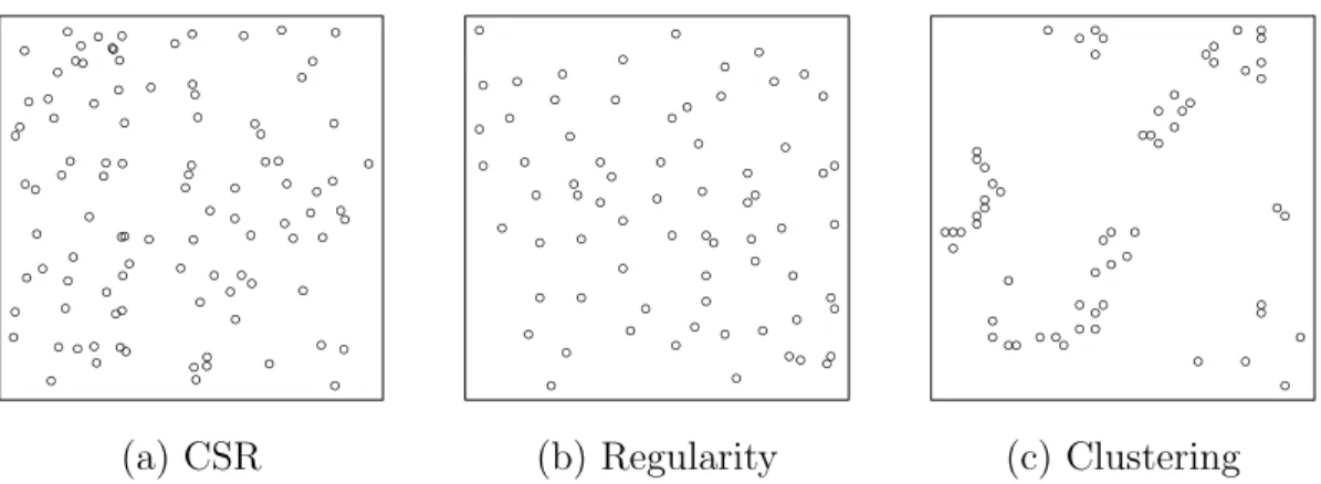
1.1 Examples of point patterns exhibiting (a) CSR, (b) regularity, and (c)

clustering. . . 4

2.1 Plots of (a) the Japanese pines data and (b) the prior and posterior

distributions for λ. The vertical line in (b) denotes the MLE ˆλ= 2.001. 16

2.2 (a) The posterior distribution for N(D), (b) the subset A ⊂ D of

interest, and (c) the posterior distribution forN(A). The solid vertical

lines in (a) and (c) represent the posterior mean and 95% credible

intervals and the dashed lines represent the observed values. . . 18

2.3 Posterior estimates for (a) F(d), (b) G(d), and (c) K(d) under the

HPP model for the Japanese black pines data. The theoretical forms

use the MLE for ˆλ and the empirical estimates are the standard

non-parametric estimates. The shaded area represents the 95% pointwise

credible intervals forK(d). . . 30

2.4 (a) The locations of 530 American sweetgum trees in a tract of Duke

forest and (b) the elevation in meters over the same region. . . 31

2.5 Posterior distributions for the parameters of the NHPP model. The

posterior mean is marked by the solid vertical line and the 95% credible

intervals are marked by the dashed lines. . . 33

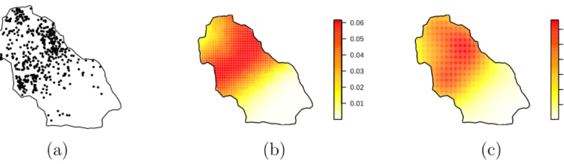
2.6 (a) The Duke forest data, (b) the posterior mean of the intensity

surface for the NHPP model, and (c) the kernel intensity estimate. . 34

2.7 The posterior distributions for (a) λ(D) and (b) N(D) in the Duke

forest NHPP model. . . 36

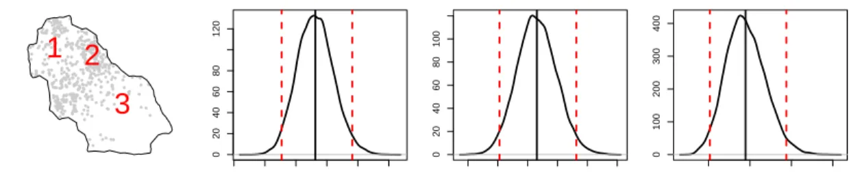
2.8 The posterior distributions for λ(s) at three points in Duke forest.

The solid vertical lines represent the posterior means and the dashed

(11)

2.9 The posterior distributions forγ(s, s0) at three points in Duke forest. The locations of the three points are given in Figure 2.8. The solid vertical lines represent the posterior means and the dashed vertical

lines represent the 95% credible intervals. . . 37

2.10 The posterior distributions for N(A), N(B), and N(A)N(B) under

the NHPP model for the Duke forest data. The solid lines give the posterior means, the dashed lines give the 95% credible intervals, and

the dotted lines give the observed values. . . 38

2.11 The posterior distributions for the inhomogeneous K-function under

the NHPP model for the Duke forest data. The theoretical and

em-pirical estimates, as computed in spatstat, are also given. . . 44

2.12 Posterior distributions for the parameters of the LGCP model. The posterior mean is marked by the solid vertical line and the 95% credible

intervals are marked by the dashed lines. The HPP MLE ˆλ is given

by the dotted line. . . 52

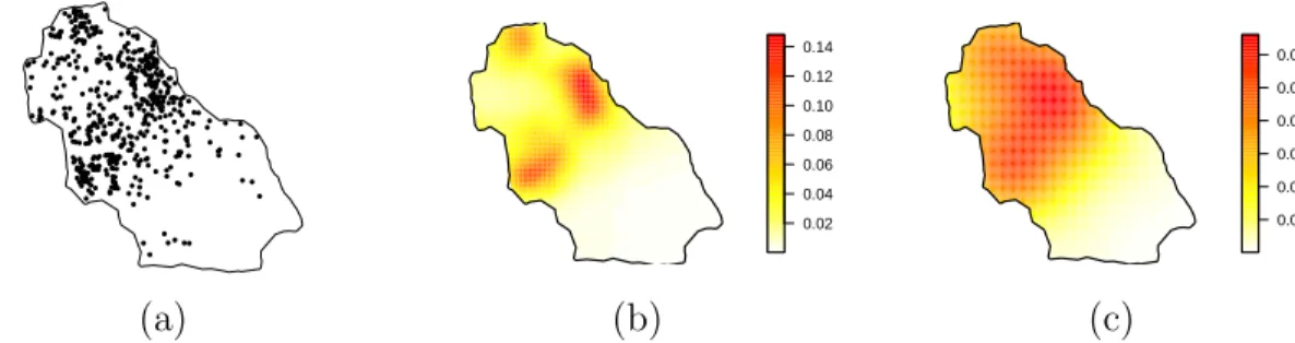
2.13 (a) The posterior mean ofλ(s) for the LGCP model and (b) the kernel

intensity estimate for the Duke forest data. . . 52

2.14 The posterior distributions for (a) λ(D) and (b) N(D) in the Duke

forest LGCP model. The observed value ofn = 530 is denoted by the

dotted line. . . 53

2.15 The posterior distributions for λ(s) at three points in Duke forest

under the LGCP model. . . 54

2.16 The posterior distributions for the second-order intensity ρ(2)₍_{s, s}0₎

and the PCF ˜g(s, s0) at each combination of the three points in Duke

forest used in Figure 2.15. . . 56

2.17 The posterior distributions for N(A), N(B), and N(A)N(B) under

the LGCP model for the Duke forest data. The solid lines, dashed lines, and dotted lines represent the posterior means, 95% credible

intervals, and observed values, respectively. . . 57

2.18 The posterior distribution for the inhomogeneous K-function under

the LGCP model for the Duke forest data. The theoretical and

em-pirical estimates, as computed in spatstat, are also given. . . 57

3.1 The raw, inverseλ, and Pearson residuals for D, A, and B under the

NHPP model for the Duke forest data, with regionsAandB as shown

in Figures 2.10 and 2.17. The dashed lines indicate the 95% credible

(12)

3.2 The raw, inverseλ, and Pearson residuals for D, A, and B under the

LGCP model for the Duke forest data, with regionsAandB as shown

in Figures 2.10 and 2.17. The dashed lines indicate the 95% credible

intervals, with 0 marked by a solid line. . . 63

3.3 Posterior mean of the smoothed raw innovation fields for the (a) NHPP

and (b) LGCP models and posterior coverage plots for the smoothed raw innovation fields for the (c) NHPP and (d) LGCP models. The coverage plots describe whether a pointwise credible interval (CI)

con-tains 0 or whether the interval is completely above or below 0. . . 67

3.4 The (a) training and (b) test data for the p = 0.5 cross-validation

data, along with the posterior means forλtrain(s) under the (c) NHPP

model and (d) LGCP model. Sincep= 0.5,λtrain₍_s_{) =}_λtest₍_s_{). . . . .} ₇₃

3.5 Ranked probability scores for the NHPP model (solid black line) and

the three LGCP models (dashed lines) fitted to the Duke forest test

data for three cross-validation sets withp= 0.5. . . 78

3.6 90% predictive interval coverage for the NHPP model (solid black line)

and the three LGCP models (dashed lines) fitted to the Duke forest

for three cross-validation sets with p = 0.5. The black dotted line

indicates the 90% nominal level. . . 79

3.7 The relative RPS for the simulated HPP data with _E[n] = 100. The

models are labeled as (A) HPP, (B) NHPP, (C) LGCP with

exponen-tial covariance, (D) LGCP with Mat´ern (ν = 3/2) covariance, and (E)

LGCP with Gaussian covariance. . . 82

3.8 The relative RPS for the simulated LGCP (exponential covariance)

data with_E[n]≈ 100 (top row) and _E[n]≈ 1000 (bottom row). The

model labels are the same as those used in Figure 3.7. . . 83

4.1 Plots of Messor ant nests (inhibitive), redwood seedlings (clustered),

and simulated homogeneous Poisson point patterns (completely

spa-tially random). . . 87

4.2 Variance metrics for simulated HPP(λ = 100) data with _E[n] ≈

100,1000. The top row shows the results when fitting the HPP model

to the HPP data and the second row shows the results using the Strauss model. The dashed line indicates the observed variance metrics. 96

(13)

4.3 Variance metrics for simulated Strauss(β = 250, γ = 0.05, R = 0.05)

data with _E[n] ≈ 100,1000. The top row shows the results when

fitting the HPP model to the Strauss data and the second row shows the results using the Strauss model. The dashed line indicates the

observed variance metrics. . . 97

4.4 Plots of (a) the Swedish pines data, (b) profile pseudolikelihood for

the Strauss model as a function of R, and (c) the (sorted) nearest

neighbor distances. The dashed line in (b) indicates the profile

max-imum pseudolikelihood estimate ˆR = 0.72. The dashed lines in (c)

indicate the candidateR values of 0.25, 0.45, 0.55, and 0.72. . . 98

4.5 Plots of (a) the Swedish pines data with subregion Alabeled and the

posterior distributions for (b–c) n and N(A) under the HPP model,

and (d–f) γ, n, and N(A) under the Strauss(R=0.72) model. The

solid and dashed lines indicate the posterior means and 95% credi-ble intervals, respectively, and the dotted lines indicate the observed

values. . . 100

4.6 Plots of theF-, G-, and K-functions for the Strauss model with R=

0.72. The theoretical forms use the MLE for ˆλ and the empirical

estimates are the standard nonparametric estimates. The shaded area

in (c) represents the 95% pointwise credible intervals for K(d). . . 100

4.7 Plots of the variance of box counts for the HPP and Strauss (R= 0.72)

model. The dashed lines indicate the observed variance, while the histogram and gray lines indicate predictive values under the model. . 101

4.8 Relative RPS at each value of q for simulated HPP data with _E[n] =

100, 1000. The LGCP (top row) and PGP (bottom row) models are

compared to the HPP model, with the horizontal line at 1 indicating

equivalent performance. . . 111

4.9 Relative RPS at each value ofqfor simulated LGCP data with_E[n] =

100, 1000. The HPP (top row) and PGP (bottom row) models are

compared to the LGCP model, with the horizontal line at 1 indicating

equivalent performance. . . 112

4.10 Relative RPS at each value of q for simulated PGP data with _E[n] =

100, 1000. The HPP (top row) and LGCP (bottom row) models are

compared to the PGP model, with the horizontal line at 1 indicating

(14)

4.11 The posterior mean intensity for the three models fit to the first

cross-validation set from the redwood tree data for p = 0.75. The circles

denoted points in the training data and the x’s represent the test data. 115 4.12 The average RPS and coverage for each model over 10 rounds of

cross-validation. The solid line is the HPP model, the dashed line is the LGCP model, and the dotted line is the PGP model. . . 116 4.13 Ranked probability scores for test data in four cross-validation sets of

the redwood data for p= 0.5, 0.75. The solid line is the HPP model,

the dashed line is the LGCP model, the dotted line is the PGP model. 117

4.14 The modified redwood seedling dataset (n = 152), which was

con-structed by improving the clustering and randomly adding 90 data points to the clusters of the original dataset in Figure 4.14. . . 118 4.15 The average RPS and coverage for each model over 10 rounds of

cross-validation for the modified redwood data. The solid line is the HPP model, the dashed line is the LGCP model, and the dotted line is the PGP model. . . 118 B.1 The RPS and coverage results for the simulated HPP data. All the

models perform fairly similarly to the HPP model. The coverage

rel-ative RPS plots show more variability as q gets larger. The coverage

levels are all close to the nominal 90% level, though with more

vari-ability in the _E[n] = 100 case. . . 133

B.2 The RPS and coverage results for the simulated NHPP data. The HPP performs poorly, but the other models perform similarly. For

E[n] ≈ 1000, the LGCP models outperform the true NHPP model

both in RPS and coverage, and the NHPP coverage is largely inade-quate despite being the true underlying model. . . 134 B.3 The RPS and coverage results for the simulated LGCP (Exponential

covariance) data. The HPP and NHPP models performed worse than

the LGCP models, especially for _E[n] ≈1000. The LGCP models all

performed very similarly, with the coverage levels sometimes dropping

close to 50%. . . 135

B.4 The RPS and coverage results for the simulated LGCP (Mat´ern ν =

3/2 covariance) data. The results are similar to Figure B.3. . . 136

B.5 The RPS and coverage results for the simulated LGCP (Gaussian covariance) data. The results are similar to Figure B.3. . . 137

(15)

List of Abbreviations and Symbols

Symbols

N(A) The number of points falling in a set A

|A| The size of a set A

λ(s) The intensity function at a location s∈D

γ(s, s0) The second-order moment measure, evaluated at s and s0

˜

g(s, s0) The pair correlation function, evaluated at s and s0

Abbreviations

CSR Complete spatial randomness

HPP Homogeneous Poisson process

GP Gaussian process

LGCP Log-Gaussian Cox process

MCMC Markov chain Monte Carlo

MLE Maximum likelihood estimate

MPLE Maximum pseudolikelihood estimate

NHPP Nonhomogeneous Poisson process

PCF Pair correlation function

PGP Poisson-gamma process

RPS Ranked probability score

(16)

Acknowledgements

First, I would like to thank my advisor, Alan Gelfand, for his dedication to my re-search and to my development as a statistician. He has provided wonderful guidance and constant encouragement over the last four years. I would also like to thank the rest of my committee, Robert Wolpert, Merlise Clyde, and Jim Clark for their time and feedback. I am also thankful for the chance to work on other projects with David Holland, Jenica Allen, and John Silander, Jr.

I am very grateful to the faculty, students, and staff who all contribute to the great environment in the department. I am thankful to have so many great fellow students who have carried me through measure theory, pulled the occasional prank on me, and provided a great source of friendship over the years.

I would like to thank my parents for their support and encouragement over my lifetime and all 20+ years of school. I would also like to thank my son, Dane, for always putting a smile on my face and providing me with fun-filled escapes from writing my dissertation. Lastly, and most importantly, I would like to thank my wife, Alyse, for her constant support and encouragement and for patiently waiting all this time for me to finally have a real job and a decent income.

This work was supported by NIH award 2R01-ES014843-04A1. I am also grateful to the International Society for Bayesian Analysis, American Statistical Association, Duke University Graduate School, and Duke University Department of Statistical Science for conference travel support.

(17)

1

Introduction

As discussed in Banerjee et al. (2014), spatial data sets are generally classified into three categories: point-referenced data, areal data, and point pattern data. The first class, point-referenced data, refers to situations where the outcome of interest

y(s) varies continuously over locationss within some regionD. Data is collected at a

finite set of locations, from which the continuous surface is then estimated. Examples of such data include estimating pollution or temperature levels across some region, such as the United States, or collecting house price information to understand the average house price in some city, state, etc. The region of interest is generally taken

to be some subset of_R2 or_R3, though higher dimensions or more abstract spaces can

be employed. Models for such data, often termed geostatistical models due to their use in many geological applications, generally employ Gaussian processes or splines as a flexible model for the continuous response surface.

Areal data differs from point-referenced data in that the spatial locations are discrete partitions of the region of interest or points on a lattice. For example, the data could consist of grayscale levels at each pixel of an image or cancer incidence

(18)

locations, though the definition of closeness must be defined for each application. Generally a local structure is defined, often employing Markov random fields, to account for the spatial correlation.

Point pattern data, the subject of this work, describes data in which random events are observed over some domain, with the number and locations of these events being random. Analysis of this category of data involves understanding the under-lying process generating these events, which includes learning whether events (also called points) are more likely to occur in certain regions of the domain and whether the existence of an event affects the locations of subsequent events. For example, a point pattern may consist of the locations of trees in a forest or the locations of fast food locations in a city. There may be extra information attached to the event, such as the type of tree or the diameter of the tree, which can enrich the analysis.

The first two classes of spatial data problems are well-studied, but the com-plexities introduced in point pattern analysis leave many open problems, such as model diagnostics and model selection for point patterns. This thesis will explore some of these issues and suggest some methods for analyzing point pattern models and enriching the inference available from these models, primarily from a Bayesian perspective.

1.1 Point patterns

Before describing our contributions, some notation and theoretical development will be given. Many resources can provide a lengthier and more rigorous devel-opment of point pattern theory and related topics; see, e.g., Cressie (1993); Banerjee et al. (2014); Gelfand et al. (2010); Illian et al. (2008); Diggle (1983); Møller and Waagepetersen (2007); Daley and Vere-Jones (1998).

As previously described, a point pattern is a collection of points or events observed over some region, with the locations and number of events both being random. Point

(19)

patterns can represent cancer cases in a region, trees in a forest, or crimes in a city. Point pattern analysis is concerned with understanding the underlying process generating the events. This involves learning about the number of events expected to occur, how likely points are to occur over different areas of the domain, and whether event locations are independent of each other. A point process will denote the underlying process which generates the observed point patterns.

The locations of the points in the point pattern will be denoted by si and the

domain of interest will be denoted byD. The collection of points makes up the point

pattern, S, with S ={si}ni=1, where n ≡N(D) is the number of points observed in

D. In general, the number of points in any set A ⊆ D will be denoted by N(A).

The treatment here will generally take D to be a subset of _R2_{, though other forms}

for D are common. Time series point patterns will often use D≡ (0, T) ⊂_R+ _and

spatiotemporal point patterns will takeD⊂_R2_×

R+. Ang et al. (2012) model crimes

on the streets in Chicago, where D is taken to be the linear network of streets in a

neighborhood of Chicago.

The least complex point patterns exhibit complete spatial randomness (CSR),

a property under which point locations occur independently and uniformly over D.

Complete spatial randomness implies that points occur with equal likelihood over

each region in D and that the points do not cluster nor repel each other. Figure 1.1

shows an example of a point pattern which exhibits CSR and two examples which violate CSR due to regularity and clustering. The clustered point pattern in 1.1c is easily distinguished from the point pattern exhibiting CSR in 1.1a. The regular point pattern in 1.1b is harder to distinguish from 1.1a, especially for untrained eyes. The main difference is that, under CSR, points will sometimes randomly occur very close to each other, while under regularity, such occurrences are rare.

Building a probabilistic model for a point pattern S requires specifying

(20)

● ● ● ● ● ● ● ● ● ● ● ● ● ● ● ● ● ● ● ● ● ● ● ● ● ● ● ● ● ● ● ● ● ● ● ● ● ● ● ● ● ● ● ● ● ● ● ● ● ● ● ● ● ● ● ● ● ● ● ● ● ● ● ● ● ● ● ● ● ● ● ● ● ● ● ● ● ● ● ● ● ● ● ● ● ● ● ● ● ● ● ● ● ● ● ● ● ● ● ● ● ● ● ● ● ● ● ● ● ● ● ● ● ● ● ● ● ● ● ● ● ● ● ● ● ● ● ● ● ● ● ● ● ● ● ● ● ● ● ● ● ● ● ● ● ● ● ● ● ● ● ● ● ● ● ● ● ● ● ● ● ● ● ● ● ●● ● ● ● ● ● ●● ● ● ●● ● ● ● ● ● ● ● ● ● ● ●●_● ● ● ● ●● ●● ● ●● ●● ● ●_● ● ● ● ●_● ● ● ● ● ●● ●● ●● ● ● ● ● ● ● ●● ● ● ● ●

(a) CSR (b) Regularity (c) Clustering

Figure 1.1: Examples of point patterns exhibiting (a) CSR, (b) regularity, and (c)

clustering.

cover the set {0,1, . . . ,∞} and is usually taken to be the Poisson distribution. The

distribution for the locations of the points must have a valid densityfθ

n for anynand

point process parameters θ. Since the points are unordered and, for now, unlabeled,

the location density fθ

n(s1, s2, . . . , sn) must be symmetric in its inputs. Combining

these two pieces, the density forS, fS, will take the form

fS(S;θ) = Pr

N(D) =n|θn!f_nθ(s1, s2, . . . , sn), (1.1)

where the factorial n! comes from the exchangeability of the events s within S.

Under CSR, the location density fθ

n is uniform and points occur independently,

leading to fθ n(s1, s2, . . . , sn) = Q if1θ(si) = Q i1/|D|= |D|

−n_{, where} _|_A_| _{denotes the}

size of a set A. Complete spatial randomness impliesstationarity, which means that

fθ

n(s1, . . . , sn) = fnθ(s1 +h, . . . , sn +h) for all n, s ∈ D ⊆ Rd and h ∈ Rd. One

implication of stationarity is that the first-order trend is constant.

The homogeneous Poisson process (HPP) is a point process that is built upon

CSR. HPPs have a single parameter λ which relates to the total number of points

expected to be observed inD. The key property of the homogeneous Poisson process

is that for any regionA ⊆D, the number of points expected inA, denoted byN(A),

(21)

number of points observed inD, has expectationλ|D|. The independence of locations

arising CSR property of HPPs implies that for two disjoint subsets, A, B ⊂ D, the

number of points occurring inAandB are independent Poisson variables, again with

expectations λ|A| and λ|B|, respectively. The HPP is clearly a stationary process,

though other stationary processes do exist.

The likelihood for a homogeneous Poisson process is composed of the two pieces

discussed previously. The random number of events observed, n, is modeled as a

Poisson random variable with expectationλ|D|. The random locations of these points

given n are distributed independently over D with density fθ

n(s1, . . . , sn) = |D|−n.

Combining these two pieces with (1.1) gives the HPP likelihood function

fS(S;λ) = e−λ|D|₍_λ_|_D_|₎n n! × n! |D|n =e −λ|D| λn. (1.2)

The parameter λfrom above is called the intensity and controls the rate at which

events occur. The intensity can be written more generally as a functionλ(s) for any

location s ∈ D, where regions with higher λ(s) have a higher expected number of

events. The general definition for the intensity function is that the intensity λ(s) is

the function satisfying _E[N(A)] = R_Aλ(s)ds for any subset A ⊆ D. The intensity

can equivalently be defined asλ(s)≡lim|∂s|→0E

N(∂s)/|∂s|. The intensity function

may not always be tractable, e.g., as in Gibbs processes, which will be discussed later. Relaxing the homogeneous Poisson process to have a spatially varying intensity

λ(s) results in the nonhomogeneous Poisson process (NHPP), also called the

inho-mogeneous Poisson process. Under the NHPP model, which is no longer stationary,

the quantity N(A) is distributed as Poisson(λ(A)) where λ(A) ≡ R

Aλ(s)ds. As

before, N(A) and N(B) are still independent, conditional on λ(s), if A and B are

disjoint subsets of D. The spatially varying intensity may include a regression

(22)

λ, whereas nowθ may be comprised ofλ0, severalβk, and possibly other parameters.

Therefore, λ(s) implicitly depends on θ, so we will generally write λ(s) but could

more explicitly write λθ₍_s_{) instead.}

The location density for an NHPP is easily developed first from considering a

single point s∗. The likelihood of the location of s∗ is relative to the height of λ(s)

at each s ∈ D. Therefore, λ(s) can be seen as the unnormalized location density,

implying that f₁θ(s∗) = λ(s∗)/λ(D), where λ(D) = R_Dλ(s)ds is the normalizing

constant. Since the NHPP still preserves independence among the locations of its

points, fθ n(s1, s2, . . . , sn) = Q si∈S λ(si)/λ(D)

. Using this and the fact that N(D)

is distributed as Poisson(λ(D)), the NHPP likelihood builds on (1.2) to become

fS(S;θ) = exp{−λθ₍_D₎_} _λθ₍_D₎n n! ×n! Y si∈S λθ₍_s i) λθ₍_D₎ = exp{−λ θ₍_D₎_}Y si∈S λθ(si) (1.3)

Continuing to relax the assumptions of the Poisson process results in more com-plex, and perhaps more useful, point processes. For example, a Cox process results

by taking the inhomogeneous Poisson process and letting λ(s) be a realization of a

random process. Gibbs processes, cluster processes, and others result when a de-pendence structure is introduced among the points. For example, saplings tend to cluster around the parent tree, resulting in a cluster process. Of course, some pro-cesses may exhibit both a nonconstant intensity as well as a dependence structure among the points, though it is known to be difficult to clearly separate these two influences, as noted in, e.g., Baddeley et al. (2000).

Point processes can be characterized by moment measures, with the intensity

function λ(s) defining the first-order moment measure of a point process. The

second-order moment measure γ(s, s0), also called the second-order intensity,

ad-dresses the covariance structure, just as a Gaussian process used in a geostatistical

(23)

satisfy-ing _E[N(A)N(B)] = R_AR_Bγ(s, s0)ds0ds, which provides a sense of the covariation

between two sets A, B ⊆ D. The pair correlation function (PCF), also called the

reweighted second-order intensity, provides a standardized version of the second-order measure, which is useful in assessing the range of correlation in point patterns (see, e.g., Illian et al., 2008, p. 220). The PCF is defined as ˜g(s, s0) =γ(s, s0)/(λ(s)λ(s0)).

Many processes have closed forms for γ(s, s0) and ˜g(s, s0), but they will not be given

here.

1.2 Frequentist Inference for Spatial Point Processes

We shall primarily operate within the Bayesian paradigm but it will be useful to briefly highlight a few aspects of frequentist inference for point patterns. As dis-cussed in Møller and Waagepetersen (2007), maximum likelihood estimates (MLEs) are not always computationally feasible for point patterns. For example, Gibbs pro-cesses (see Section 4.1), have unknown normalizing constants, though path sampling (Gelman and Meng, 1998) and MCMC methods (Ogata and Tanemura, 1981) have developed to achieve MLE estimates. The MLEs of spatial point processes do not enjoy the usual asymptotic properties, making them less dominant over other meth-ods. See Møller and Waagepetersen (2007, 2003) and references therein for a more thorough discussion of maximum likelihood estimates for point processes. In some cases, however, the MLE is simple to obtain. For example, the MLE does exist for

the intensity parameter λ of an HPP, and is simply ˆλ=n/|D|.

Since point process MLEs do not enjoy the usual asymptotic theoretical support for MLEs (Baddeley and Turner, 2000), other estimation methods enjoy wide use. For some point processes, minimum contrast estimates provide robust, computationally-efficient estimates through matching higher-order properties of the process to the

observed data. Let T(r;θ) be some summary statistic of the point process with

(24)

to be the pairwise correlation function or the K-function, which will be introduced

in Chapter 2. If the PCF ˜g(s, s0) is just a function of the distance r = ||s−s0||

and then we can take T(r;theta) to be the PCF evaluated atr. Then the minimum

contrast estimate ˆθ is the parameter (or set of parameters) θ which minimize

Z rmax

rmin

ˆ

T(r)q−T(r;θ)qpdr, (1.4)

where p, q > 0 and 0 ≤rmin < rmax specifies a reasonable range of values for r. See

Waagepetersen (2007) for further discussion.

For processes with a likelihood containing an intractable normalizing constant, such as Gibbs processes, the pseudolikelihood is often employed because it removes the need to estimate the normalizing constant. Besag (1977) defines the point process pseudolikelihood to be P L(θ;S) = exp − Z D λθ(s;S)ds Y si∈S λθ(si;S), (1.5)

whereλθ(s;S) is the (Papangelou) conditional intensity of at s∈D and depends on

process parameters θ. The conditional intensity is defined as

λθ(s;S) =            fθ(S∪ {s}) fθ₍_S₎ s 6∈S, and fθ₍_S₎ fθ₍_S_{\ {}_s_}₎ s ∈S, (1.6)

where fθ _{is the location density and} _S_{\ {}_s_} _denotes _S _{with the singleton point}

s removed. For Poisson processes, where point locations occur independently, the

conditional intensity is equal to the intensity, orλθ(s;S) =λθ(s). For processes with

a second-order dependence, the conditional intensity will differ from the intensity according to the nature of interactions among points specified by the process. For

(25)

example, in a cluster process, λθ₍_s_;_S_{) may be larger than} _λθ₍_s_{) if}_s _{is close to some}

of the points inS.

The real benefit to using the pseudolikelihood is that the normalizing constant cancels out in the fraction in (1.6) when computing the conditional intensity. This is because both the numerator and denominator have the same intractable normalizing

constant because the parameters in fθ are the same. The point process model can

then be written as a generalized linear model and fit using a Berman-Turner device (Berman and Turner, 1992; Baddeley and Turner, 2000). The fitted model param-eters are the maximum pseudolikelihood estimates (MPLEs). Baddeley and Turner (2000) notes that MPLEs are consistent and asymptotically normal under suitable conditions. Huang and Ogata (1999) suggest obtaining the MPLEs and then taking a single Newton-Raphson step toward maximizing the likelihood.

1.3 Bayesian Inference for Spatial Point Processes

In brief, Bayesian modeling seeks to take prior belief about model parameters θ,

quantified by a prior distributionπ(θ), and combine this prior belief with the observed

datayto provide an updated belief aboutθ. This updated belief, called the posterior

distribution π(θ|y), is a probability distribution which accounts for the information

about θ in both the prior and the data using Bayes rule. The posterior distribution

is calculated as

π(θ|y) = Rp(y|θ)π(θ)

Θp(y|θ)π(θ)

, (1.7)

where p(y|θ) is the data model, which is equivalent to the likelihood L(θ;y), and θ

can take on values over some domain Θ. Though the integral in the denominator is generally intractable, methods such as Gibbs sampling and the Metropolis-Hastings

(26)

chain Monte Carlo (MCMC). More development on the basics of Bayesian inference is given in, e.g., Gelman et al. (2013).

Bayesian modeling can be challenging for spatial point processes, due to the same issues with an intractable normalizing constant in the point process likelihood as dis-cussed above, but also due to poor mixing properties and inefficiency when applying standard MCMC algorithms. Fortunately, most point process models have at least one working method for obtaining posterior distributions for the model parameters, often involving an advanced MCMC algorithm. These methods will not be discussed here, but rather presented as they are used in the ensuing chapters.

Our focus will be less on how to fit Bayesian models and more on what to

do once we’ve fit them. We will often use the Bayesian framework to generate

posterior predictive distributions of point patterns. The posterior predictive

dis-tribution takes the posterior disdis-tribution π(θ|y) and generates simulated data y∗

using the model. The posterior predictive distribution is written as p(y∗|y) where

p(y∗|y) = R_Θp(y∗|θ)π(θ|y)dθ. Drawing from the posterior predictive distributions

provides replicatesy∗ which are directly comparable to the original data y.

1.4 Contributions to Spatial Point Process Analysis

Typical point pattern analysis usually begins by exploring whether such a point pattern exhibits complete spatial randomness (i.e., whether the point pattern arose from an HPP). Complete spatial randomness is violated if events exhibit a depen-dence structure and/or they occur with nonconstant intensity. Once CSR has been rejected for a given point pattern, however, the next model chosen should similarly be subjected to scrutiny and compared with other valid models. This second set of analyses is usually not carried out quite as thoroughly as the initial analysis which rejected CSR.

(27)

The gap in analysis here is more attributable to a lack of powerful diagnostic and comparison methods than to a lack of effort. Testing goodness of fit is not straight-forward for point patterns, nor is there a widely applicable, easy-to-use method for model selection. The challenge with point patterns, as shall be presented in this work, is that a point pattern contains limited information about the process which generated it. For example, learning about intensity function is difficult because the smoothness in the intensity estimate is largely determined by the imposed model, since the data provide little indication of the smoothness of the original process. The user must either have prior knowledge of the smoothness or must employ some metric to choose an optimal smoothness parameter, as is done in kernel density estimation. Chapter 2 describes point pattern analysis for Poisson processes and log-Gaussian Cox processes. Details about fitting Bayesian models for each are given, followed by a discussion of many posterior summaries which can be generated for a richer analysis of the posterior distribution. Much of this relies on generating posterior predictive point patterns from the posterior distributions of the model parameters to create

model-based summaries of interest. Obtaining model-based estimates of theF-, G-,

and K-functions are discussed and compared to the usual nonparametric estimates.

Chapter 3 builds on the model-based summaries of Chapter 2 to discuss ideas for model diagnostics based on the posterior predictive point patterns. The proposed

predictive residuals are shown to illuminate regions ofDwhere the model fits poorly

and, if the regions are substantial enough, can indicate overall lack of fit. For models that seem to adequately fit the data, a similar approach allows us to apply proper scoring rules to compare models. Cross-validation ideas presented herein allow for model comparison on data not used to fit the model. A large simulation study illuminates the extent of learning available when comparing point process models.

Chapter 4 extends the ideas of Chapters 2 and 3 to more complex processes, such as Gibbs processes and cluster processes. First, adaptations for Gibbs processes

(28)

are presented to overcome the inherent dependence structure among points. Since cross-validation is not viable for Gibbs processes, posterior predictive checks (Gelman et al., 1996) are utilized to determine model fit. The discussion then moves on to cluster processes, for which the methods of Chapter 3 apply. Ideas are then given for other complex point processes, with some discussion of posterior inference and model assessment.

Finally, Chapter 5 will summarize the work presented herein and discuss potential paths for future research and improvement of these methods.

(29)

2

Bayesian Point Pattern Analysis

This chapter details Bayesian model-fitting for many standard point processes and introduces methods for extensive posterior inference. Beginning with homogeneous point processes, we illustrate how the posterior distribution for the model provides a rich variety of options for posterior inference using posterior predictive point pat-terns. Later in the chapter, models for nonhomogeneous point processes will be introduced and these posterior inference methods will naturally lead themselves to further analysis.

The goal with our posterior inference is to provide model-based inference of

pos-terior quantities of interest. For example, Ripley’s K-function (Ripley, 1976; Dixon,

2002) is a common exploratory tool in point pattern analysis which describes the

expected number of points within a distance d of a typical point in the point

pat-tern. It is commonly used to criticize the CSR hypothesis by comparing the observed

distribution of the K-function to its theoretical distribution under CSR. The usual

K-function estimate employs a nonparametric estimate of the intensity surface, but

we will take a model-based approach and use our posterior draws for the intensity surface instead. Our methods will demonstrate how to provide a whole posterior

(30)

distribution for theK-function, so that a comparison to the theoretical value can be done with a knowledge of the uncertainty involved.

2.1 Homogeneous Poisson Processes

As noted in the previous chapter, the most basic point process is a homogeneous Poisson process (HPP). This process implies that events occur independently over

the domain with constant intensity. This model has a single parameter λ which

defines the number of events in any region A ⊆ D to be distributed as N(A) ∼

Poisson(λ|A|). With one parameter, fitting an HPP model is very simple. From a

frequentist perspective, the maximum likelihood estimate (MLE) is just the number

of observed events divided by the area of D, or ˆλ = n/|D|. This is easily derived

from the HPP likelihood, given in (1.2).

A Bayesian model requires a prior distribution for λ. The gamma distribution, a

flexible distribution over _R+_{, provides a conjugate prior for} _λ_{. Taking the prior for}

λ to be

λ∼Gamma(aλ, bλ), (2.1)

with prior expectation _E[λ] =aλ/bλ, the posterior is given by

λ|S∼Gamma(aλ+n, bλ+|D|). (2.2)

Since the posterior distribution for λ has a closed form, there is no need for

MCMC. With little prior knowledge about the process, one could also use the Jeffreys

prior, which would set the prior forλasp(λ)∝1/λ. The Jeffreys prior results in the

posterior Gamma(n,|D|). We imagine that informative prior knowledge is generally

available, whether it be an expected number of trees per hectare or cancer cases per geographic region.

Other prior distributions for λ, such as the log-normal distribution, may also

(31)

algo-rithm. In fact, one could alternatively reparameterize fromλto exp{β0}and employ

a prior on β0 that takes values over R. For example, a normal prior could be used

for β0, which induces a log-normal prior for λ. No matter the prior for λ, we can

easily obtain posterior draws for λ and use them in posterior analysis.

2.1.1 Japanese Pines Data

To illustrate the HPP model, we turn to a well-studied dataset consisting of the

locations of 65 black pine saplings in a 5.7m × 5.7m square patch of forest. This

dataset was first studied by Numata (1961) but has seen several follow-up analyses (Diggle, 1983; Ogata and Tanemura, 1981; Baddeley and Turner, 2000). A plot of the data is given in Figure 2.1a. The data seem to be evenly spread over the domain, suggesting that a homogeneous intensity is reasonable.

To fit the HPP model, we use a gamma prior forλas suggested in (2.1). The prior

distribution forλcan then be specified directly or can be induced by first specifying a

prior over the expected number of trees _E[N(D)] = λ|D|. Suppose our prior belief is

that the expected number of trees in the region is about 70 trees with a prior variance

of 100. This puts most of the prior mass for _E[N(D)] between about 45 trees and

95 trees. Using a gamma distribution for _E[N(D)], the expected value and variance

choices imply that _E[N(D)] ∼Gamma(49, 0.7). Since _E[N(D)] = λ(D) = λ|D| for

an HPP, this prior for the expected number of trees can be easily converted into a

prior for λ itself. The prior λ|D| ∼ Gamma(49, 0.7) implies the prior distribution

for λ isλ ∼ Gamma(aλ = 49, bλ = 0.7|D| = 22.743). This gives a prior mean for λ

of 2.154 with variance of 0.095.

This prior for λprovides the posterior distribution forλ as Gamma(114, 55.233),

with posterior mean _E[λ|S] = 2.064. The prior and posterior distributions for λ for

(32)

● ● ● ● ● ● ● ● ● ● ● ● ● ● ● ● ● ● ● ● ●●● ● ● ● ● ●● ● ●● ● ● ● ● ● ● ●● ● ● _● ● ● ● ● ● ● ● ● ● ● ●● ● ● ● ● ● ● ● ● ● ● 0 1 2 3 4 5 0 1 2 3 4 5 1.0 1.5 2.0 2.5 3.0 3.5 0.0 0.5 1.0 1.5 2.0 dgamma(xseq, a.lam, b .lam) Prior Posterior (a) (b)

Figure 2.1: Plots of (a) the Japanese pines data and (b) the prior and posterior

distributions forλ. The vertical line in (b) denotes the MLE ˆλ = 2.001.

MLE ˆλ= 2.001. For any subregion of interest A⊆D, the posterior distribution for

λ(A) is λ(A)∼Gamma(aλ+n,(bλ+|D|)/|A|).

2.1.2 Posterior Analysis for HPPs

We now show that the Bayesian modeling framework lends itself naturally to a rich class of posterior model summaries. Not only do we have posterior draws of our parameters, which we can use to recreate the intensity surface, but we can also use these posterior draws to simulate posterior predictive point patterns, denoted by

{S_l∗}L

l=1. The posterior predictive point patterns will reflect our uncertainty in our

model parameters and will be helpful in summarizing the model’s fit to the data. In Chapter 3, we will discuss model diagnostics and model selection for point process models.

The first basic question that might be asked after fitting the model is how many

points should be expected in the domain D. As noted previously, the expected

number of points in D, denoted by _E[N(D)] (or, equivalently, _E[n]), is given by the

quantityλ(D), which is equal toλ|D|for an HPP. The posterior distribution ofλ(D)

is Gamma(aλ+n,(bλ+|D|)/|D|) distribution with posterior mean|D|(aλ+n)/(bλ+

(33)

specification, this distribution can in general be approximated using the posterior

draws for λ and multiplying them each by |D|.

A more useful answer to this question, however, can be given by finding the

posterior predictive distribution of N(D) itself, rather than the posterior for its

ex-pected value. Denoting the posterior draws ofλby{λ(l)_}L

l=1, the posterior predictive

draws for N(D), which we’ll denote by N(l)(D), can be easily simulated from the

model. For an HPP model this only requires drawing N(l)(D) ∼ Poisson(λ(l)|D|)

for l = 1, . . . , L. L should be a large number to fully capture the variability in the

parameters and the point process itself. We will generally take L to be 1000, but

since the MCMC chain will be run for much longer than 1000 iterations, we can take

the λ(l) _{draws from the posterior to actually be thinned samples from the MCMC}

chain.

The expected value of the N(l)₍_D_{) is}

E[N(D)|S] as desired, but one can now

also provide credible intervals to quantify the posterior variability of N(D). Figure

2.2a shows the posterior distribution for the number of points in D, constructed

using the N(l)(D) draws. We see that the mean number of points in the predictive

point patterns is 67.16, which is close to the theoretical value of 67.06 and the

observed n = 65, with a 95% credible interval of (48, 88). With a full posterior

distribution, other potential summaries of interest can also be calculated, such as

P r[N(D)≥70] = 0.415.

Figure 2.2b shows a subregionAfor which we might want to know the distribution

of the number of points. Again, we could either look at the posterior distribution of

λ(A), which gives the expected number of points in A, or of N(A), the number of

points itself. We prefer to look at the posterior distribution of N(A) as it is more

tangible, though the posterior ofλ(A) has a nice closed form as given above. Posterior

draws for N(A) are drawn from N(l)₍_A₎_∼_Poisson(_λ(l)_|_A_|_{) as shown previously. The}

(34)

40 50 60 70 80 90 100 0.00 0.01 0.02 0.03 0.04 ● ● ● ● ● ● ● ● ● ● ● ● ● ● ● ● ● ● ● ● ●●● ● ● ● ● ●● ● ●● ● ● ● ● ● ● ●● ● ● ● ● ● ● ● ● ● ● ● ● ● ●● ● ● ● ● ● ● ● ● ● ● 0 1 2 3 4 5 0 1 2 3 4 5 A 0 5 10 15 0.00 0.05 0.10 0.15 (a) (b) (c)

Figure 2.2: (a) The posterior distribution for N(D), (b) the subset A ⊂ D of

interest, and (c) the posterior distribution for N(A). The solid vertical lines in (a)

and (c) represent the posterior mean and 95% credible intervals and the dashed lines represent the observed values.

a posterior mean of 8.21 with a 95% credible interval of (3, 14). The observed N(A)

is 9, so our posterior interval seems reasonable.

The posterior distribution of the second-order intensity γ(s, s0) is also available

to us. For an HPP, γ(s, s0) =λ2 _{due to the independence among the points. Draws}

from this posterior distribution are obtained by simply squaring the draws of the

intensity, λ(l). The pairwise correlation function ˜g(s, s0) is equal to 1 for an HPP,

again because of the independence, but a posterior distribution for the PCF could be obtained for more complex point patterns, as will be shown later. For two

sub-regions A, B ⊆ D, we can also obtain the posterior distribution of [N(A)N(B)].

Draws from this distribution are obtained by first taking draws from the

poste-rior distributions for N(A) and N(B) as described above and then multiplying the

draws from each: N(l)₍_A₎_×_N(l)₍_B_{). In fact, the posterior distribution any}

func-tion of subsets A1, . . . , Ak is available to us, whether it is [N(A1)N(A2). . . N(Ak)]

(35)

2.1.3 Homogeneous F-, G-, and K-functions

So far, we have been calculating these posterior quantities of interest without much theoretical justification. The main theoretical tool we can employ here is Campbell’s

Theorem (see, e.g., Banerjee et al., 2014), which gives the expectation of a D

-measurable function g of points in a point patternS. Campbell’s Theorem gives the

equality E h X si∈S g(si) i = Z D g(s)λ(s)ds. (2.3)

For a feature of interest, say g(s) = 1(s ∈ A) for some set B ⊂ D, Campbell’s

Theorem says thatP

si∈S1(si ∈A) is an unbiased estimator for

R

D1(s∈A)λ(s)ds=

R

Aλ(s)ds = λ(A), which is just the expected number of points falling in a region

A. All that is required is to choose an appropriate function g such that the

right-hand side gives a quantity of interest, then the left-right-hand side becomes the unbiased estimate of the quantity of interest. This theorem is typically used to construct

estimators as functions of the observed point pattern S. However, this theorem is

also useful when applied to posterior predictive point patterns, as we will now discuss.

With the posterior draws for λ, posterior predictive point patterns are trivially

generated by first drawing the number of points n(l) ≡ N(l)(D) in the posterior

predictive point pattern S_l∗ from n(l) _∼ _Poisson(_λ(l)_|_D_|_). _{The locations of each}

s∗_li ∈S_l∗ are then randomly generated with uniform probability over D. For irregular

D, the location sampling can be performed by repeatedly drawing points within a

bounding box for D, retaining any points which fall inside D also, and continuing

untiln(l) _{locations have been sampled.}

These posterior predictive point patterns provide an alternate, more general,

method for constructing the posterior distributions ofN(D) andN(A). For each S_l∗,

(36)

points inside Agives N(l)₍_A_{). Previously, we simply drew} _N(l)₍_D_{) and}_N(l)₍_A_{) from}

their marginal (Poisson) distribution. The two methods are comparable, though this counting method using posterior predictive point patterns will also work for more complex point patterns, such as those with spatially varying intensities and

second-order dependence. Each N(l)₍_A_{), for example, then takes the form of a sum}

which becomes the inside part of the expectation on the left-hand side (2.3). Each

of these has expectation R_D1(s∈ A)λ(l)(s)ds =λ(l)(A) using Campbell’s Theorem.

Integrating over our posterior samples, we find that the expected value of the left

side _E[N(A)|S] is equal to _E[λ(A)|S] as expected. Though the result may not be

surprising, we see how Campbell’s Theorem begins to prove useful in conjunction with these posterior predictive point patterns.

Campbell’s Theorem also has a bivariate form for a (D×D)-measurable function

g of two points inS: E h _X si, sj∈S i6=j g(si, sj) i = Z D Z D g(s, s0)γ(s, s0)ds ds0, (2.4)

where γ(s, s0) is the second-order intensity defined previously. The bivariate form is

useful for exploring second-order properties of a point process. Another useful result is the Georgii-Nguyen-Zessin (GNZ) formula (Georgii, 1976; Nguyen and Zessin, 1979), which gives the equality

E X si∈S g(si, S\{si}) =_E Z D g(s, S)λ(s;S)ds , (2.5)

whereλ(s;S) is the Papangelou conditional intensity andgis a non-negative function.

We can now use these results to obtain inference for the homogeneous F-, G-,

and K-functions. These three functions are standard procedures in point pattern

(37)

complete spatial randomness is a reasonable assumption for the current dataset. If

CSR seems reasonable, an HPP model is employed. Otherwise, the F-, G-, and

K-functions provide insight into whether the points appear to be more clustered or

dispersed than would be expected under CSR. Typically, nonparametric empirical estimates of these functions are used, but we demonstrate how to use these theoretical tools along with Monte Carlo integration to provide model-based expectations and posterior distributions for these functions.

The F-function, denoted byF(d), is the cumulative distribution function (CDF)

of the nearest neighbor distance d from a random point inD to an event in S. It is

often called the “empty space function” because it measures the gaps or empty space

in the point pattern. Under CSR, F(d) = 1−exp(−λπd2_{). The usual estimator for}

F(d) is obtained by randomly sampling a large number of points uniformly over D,

call this set of pointsT ={tj}Jj=1, and calculating the proportion oftj having a point

of S within distance d.

The G-function, denoted by G(d), is the CDF of the nearest neighbor distance

from one observed event to another. Under CSR, G(d) = F(d) = 1−exp(−λπd2).

Using the notation of Banerjee et al. (2014), define N(s, d, S) to be the number of

events in S\s inside a ball of radius d centered around an arbitrary observed event

s, where S\s denotes the point pattern S with the event at s removed. In this

notation, we can express G(d) as P r[N(s, d, S)>0].

The K-function, also called Ripley’sK-function, gives a scale-free description of

the expected number of points within distance d of an arbitrary event in S (Ripley,

1976; Dixon, 2002). For a first-order stationary process, meaning that the intensity is

constant over D, the K-function is equal to _E[N(s, d, S)]/λ. Dividing by λ adjusts

for the overall intensity of the HPP and allows K(d) to be scale-free. Under CSR,

(38)

Appendix A contains the standard empirical estimators for these functions. These estimators also include an edge correction to compensate for the bias in the naive estimators. The bias arises because these point patterns are only observed over

some finite domainD, but could potentially exist on a much larger, possibly infinite,

domain (such as _R2_{). Looking at} _K₍_d_{), for example, when counting the number of}

neighbors within distance d of some point si ∈ S, it will often be the case that si

is close to the boundary of S. When that happens, si may have neighbors that are

outside of D yet are within distance d of si. These neighbors were not observed

and therefore we have no idea of knowing how many there might be. The edge corrections proposed in the literature address this bias by adjusting the estimates

to handle points near the boundary of D differently. For example, the “reduced

sample” or border correction estimates these functions using only the points in D

that are at least distance d from the boundary of D. Since the remaining points

are far enough from the edge of D, their d-close neighbors will all be observed.

This correction provides an unbiased estimate though it sacrifices useful information. Other approaches adjust differently and are able to retain more of the data.

As noted previously, typical point pattern analysis involves obtaining the em-pirical estimate of these three functions, as well as other similar functions such the

J-function, etc. Typically this is done as an exploratory analysis, investigating what

second-order trends are suggested by the data. We now present methods for obtain-ingmodel-based posterior estimates of these functions. In the following development,

these functions describe a posteriori features of our model as opposed to just

high-lighting trends in the data.

For some models, such as the HPP model, the theoretical forms for the F-, G

-and K-functions are known and the posterior mean for model parameters, such as

λ for the HPP, could be used as plug-in estimates. However, our method employs

(39)

uncertainty in the posterior. Further, our method will generalize to other models

without requiring that the theoretical forms ofF(d), G(d), etc., be known.

We first begin by developing a model-based summary of G(d). We have been

somewhat relaxed in our notation thus far by assuming that each si in S is within

D. In order to think correctly about edge effects, however, we will assume that the

point pattern might have points outside ofD and the notation will explicitly restrict

S toDwhen desired for the rest of this section. It is often the case thatDrepresents

an observation window inside which events of interest are recorded, yet these events exist as part of a much larger point pattern. A common example of this is recording tree locations within some small subset of a large forest.

Let ND(si, d, S) ≡ N(si, d, S∩D) denote the number of points in S ∩D that

are d-close to si. Referring to the discussion above about edge corrections, we only

know quantities such as ND(si, d, S) but we would like to adjust this quantity to be

unbiased for N(si, d, S).

Recalling thatG(d) can be written as P r[N(s, d, S)>0], consider the calculation

ES X si∈S∩D 1(ND(si, d, S)>0) =EN(D)ES|N(D) X si∈S∩D 1(ND(si, d, S)>0) =_EN(D) X si∈S∩D ES|N(D)1(N(si, d, S)>0) =_EN(D) N(D)P r[ND(s, d, S)>0] =λ(D)P r[ND(s, d, S)>0]. (2.6)

We can adjust the left-hand side of (2.6) and consider the quantity

ES

X

si∈S∩D

1(ND(si, d, S)>0)

(40)

which has expected value ES X si∈S∩D 1(ND(si, d, S)>0) N(D) =EN(D) 1 N(D) X si∈S∩D ES|N(D)1(ND(si, d, S)>0) =_EN(D) P r[ND(s, d, S)>0] =P r[ND(s, d, S)>0]. (2.8)

The quantity P r[ND(s, d, S) >0] is close to G(d). In fact, removing the

expec-tation from the left-hand side of (2.7) gives a naive estimator forG(d). However, we

are still only estimating P r[ND(s, d, S) > 0], i.e., the probability that the count is

greater than 0 under the restriction of S toD. Evidently,P r[N(s, d, S)>0] applies

to the countable point pattern S over _R2 _{but we can only make the previous}

calcu-lations by restriction to a bounded setD. Of courseND(s, d, S)≤N(s, d, S) for any

s and any S, so G(d) =P r[N(s, d, S)>0]≥P r[ND(s, d, S)>0] which clarifies the

need for edge correction.

The edge correction for the usual empirical estimate considers summing over only

those si ∈ S∩D such that cd(si) ⊂ D, where cd(si) is the interior of the circle of

radius d atsi. This is also often written as only considering those si ∈ S∩D with

bi ≤ d, where bi is the distance from si to the nearest boundary of D. The edge

correction is needed because when cd(si)∩DC 6= ∅, or equivalently bi > d, si may

have a d-close neighbor just outside of D that we didn’t observe.

In this spirit, suppose we look at

ES " X si∈S∩D 1(ND(si, d, S)>0, cd(si)⊂D) N(D) # . (2.9)

(41)

Note that the sum in the numerator of (2.9) is less than that in the numerator of (2.7). Now the expectation in (2.9) is

ES " X si∈S∩D 1(ND(si, d, S)>0, cd(si)⊂D) N(D) # =P r[ND(s, d, S)>0, cd(s)⊂D]. (2.10)

Again, this describes the probability that, for a randomS, and a randoms∈S with

cd(s)⊂D, there is at least one s0 ∈(S\{s})∩D incd(s).

Let ˜G(d) = P r[ND(s, d, S)>0|cd(s)⊂D]. The usual empirical estimate obtains

an estimate of this probability and calls it ˆG(d). For us, we would say that ˜G(d) =

G(d) for small values of d, such that it is possible for cd(s) ⊂ D. The empirical

estimate will have a denominator decreasing in d, eventually becoming 0 when d is

too big, but this degenerate case is usually handling by defining ˆG(d) = 1 for such

cases.

We can easily create a Monte Carlo estimate of (2.10), so if we estimateP r[cd(s)⊂

D], the ratio will provide a Monte Carlo estimate of ˜G(d), an edge-corrected

esti-mate. Since our estimate ofP r[cd(s)⊂D] will be less than 1, we will increase (2.11),

which makes sense given that P r[ND(s, d, S) > 0, cd(s) ⊂ D] ≤ P r[ND(s, d, S) >

0] ≤ P r[N(s, d, S) > 0] = G(d). Our estimate for P r[cd(s) ⊂ D] will be based on

the equality ES X si∈S∩D 1(cd(si)⊂D) N(D) =P r[cd(s)⊂D], (2.11)

and the left-hand side of (2.11) naturally invites a Monte Carlo integration using our posterior predictive point patterns.

In summary, we will construct ˜G(d) = P r[ND(s, d, S) > 0|cd(s) ⊂ D] using

Monte Carlo integration with our posterior predictive point patterns (which we have

(42)

P r[ND(s, d, S)>0, cd(s)⊂D]≈ 1 L L X l=1 P s∗_li1(N(s ∗ li, d, S ∗ l)>0, cd(s∗li)⊂D) N(l)₍_D₎ (2.12) P r[cd(s)⊂D]≈ 1 L L X l=1 P s∗_li1(cd(s ∗ li)⊂D) N(l)₍_D₎ (2.13) ⇒G˜(d)≈ 1 L PL l=1 P s∗_li1(N(s ∗ li, d, Sl∗)>0, cd(s∗li)⊂D) N(l)₍_D₎ 1 L PL l=1 P s∗_li1(cd(s ∗ li)⊂D) N(l)₍_D₎ . (2.14)

TheF-function is very similar to theG-function, so we can use a similar argument

to construct our posterior estimate of F(d), or rather ˜F(d) = P r[ND(t, d, S) >

0|cd(t)⊂D] for any random locationt∈D. The only difference here is that we will

look at the grid pointstlinT and the distance to their nearest neighbors in eachSl∗.

The posterior estimate for ˜F(d) is then constructed as

˜ F(d)≈ 1 L PL l=1 PJ j=11(N(tj, d, S ∗ l)>0, cd(tj)⊂D) J 1 L PL l=1 PJ j=11(cd(tj)⊂D) J = 1 L PL l=1 PJ j=11(N(tj, d, Sl∗)>0, cd(tj)⊂D) Pj j=11(cd(tj)⊂D) . (2.15)

Turning now toK(d), we consider the term _ES P_s_i∈S∩DND(si, d, S)

. Following a similar argument to our calculation in (2.6), we get

ES X si∈S∩D ND(si, d, S) =λ(D)ES ND(s, d, S) . (2.16)

(43)

As before, we can adjust (2.16) to get ES X si∈S∩D ND(si, d, S) N(D) =ES ND(s, d, S) . (2.17) If we call _END(s, d, S)

=λKD(d), we have an immediate Monte Carlo

integra-tion for KD(d), i.e.,

KD(d)≈ 1 L L X l=1 " P s∗_liN(s ∗ li, d, S ∗ l) λ(l)_N(l)₍_D₎ # (2.18)

using the posterior draws λ(l) _{and posterior point patterns} _S∗

l, each drawn from an

HPP(λ(l)_).

Again, we see the need for edge correction. We are estimatingKD(d) rather than

K(d). In fact, since, again ND(s, d, S)≤N(s, d, S), we see that KD(d)≤K(d).

Now consider that P

si∈S∩DND(si, d, S) = P

si∈S∩D P

j6=i1(sj ∈ cd(si) ∩ D).

Given si, E1(cd(si)∩D) = P r[cd(si)∩D]. We want P r[cd(si)], but again we are

restricted to only observingS∩D, so we can only observe1(sj ∈cd(si)∩D). Instead,

note that

P r[cd(si)] =P r[cd(si)∩D]/P r[D|cd(si)]. (2.19)

The denominator provides the appropriate inflation of the probability to give us

P r[cd(si)].

In the literature, the empirical estimators employ an edge-correction factorwsi,sj

which is similar to P r[D|cd(si)]. The adjustment wsi,sj proposed in Ripley (1977)

calculates, for a given sj, the proportion of the circumference of the circle centered

atsi with radius||si−sj||which is contained in D. In other words,wsi,sj is a rough

approximation to P r[D|c||si−sj||(si)]. Exact expressions for wsi,sj are available for

D of special shape (in 2 dim, essentially a circle; see Illian et al., Appendix B). Yet

(44)

|D∩cd(si)|/|cd(si)|, the proportion of cd(si) that is inside D. To handle arbitrary

regions D, we must perform a Monte Carlo integration for each si ∈ S ∩D, to

perform a Monte Carlo integration, i.e., draw points uniformly in cd(si) and obtain

the proportion which also fall in D. This proportion is the Monte Carlo estimate

˜

wsi ≈ |D∩cd(si)|/|cd(si)| = |D∩cd(si)|/(πd

2_{), which can be approximated within}

arbitrary precision.

The resulting edge-adjusted estimator for N(s, d, S) would become

X si∈S∩D P j6=i1(sj ∈cd(si)∩D) ˜ wsiN(D) (2.20)

which, with posterior predictive patterns S_l∗, would yield a Monte Carlo estimator

for ES " X si∈S∩D P j6=i1(sj ∈cd(si)∩D) N(D)P r[D|cd(si)] # =_ES " X si∈S∩D ND(si, d, S) N(D)P r[D|cd(si)] # =_ES ND(s, d, S) P r[D|cd(s)] . (2.21)

Given s, we can think of ND(s, d, S) as the number of successes in N(s, d, S)

Bernoulli trials with success probabilityP r[D|cd(s)]. So,

END(s, d, S)|N(s, d, S), P r[D|cd(s)] =N(s, d, S)P r[D|cd(s)] (2.22) or_E ND(s, d, S) P r[D|cd(s)] |N(s, d, S), P r[D|cd(s)] =N(s, d, S). (2.23) Hence E ND(s, d, S) P r[D|cd(s)] =_{E E} ND(s, d, S) P r[D|cd(s)] |N(s, d, S), P r[D|cd(s)] =_EN(s, d, S). (2.24)

As above, since we want _EN(s, d, S)/λ, we will put λ(l) _{in the denominator of}

(45)

“finite”K-functionKfin(d) in (3.5.7) in Illian et al. Our resulting posterior estimator for K(d) is ˜ K(d)≈ 1 L L X l=1 X s∗_li∈S∗_l∩D P j6=i1(s ∗ lj ∈cd(s∗li)∩D) ˜ ws∗ liλ (l)_N(l)₍_D₎ , (2.25) where ˜ws∗

li is estimated through a Monte Carlo integration.

The form of the K-function also allows a posterior distribution due to the single

Monte Carlo integration taking place outside the ratio. By removing the averaging overl = 1, . . . , L, we also obtain the posterior draws forK(d), which we will denote

by ˜Kl(d) and calculate as ˜ Kl(d) = X s∗_li∈S∗_l∩D P j6=i1(s ∗ lj ∈cd(s∗li)∩D) ˜ ws∗ liλ (l)_N(l)₍_D₎ . (2.26)

This approach for generating posterior samples of the K-function is valid for any

point process with a constant intensity of a known form, such as an HPP. For a process where the intensity function is not known, such as a Strauss process, then another approach must be taken. This is one area of ongoing research.

2.1.4 F-, G-, and K-functions for Japanese Pines Data

Figure 2.3 shows the posterior estimates for ˜F(d), ˜G(d), and K(d) using the HPP

model for the black pines data from Figure 2.1a. The empirical F(d), G(d), or K(d)

functions represent the standard nonparametric empirical estimates with appropriate

edge corrections. The theoretical F(d) and G(d) represent the theoretical values

using ˆλ = n/|D| and the theoretical K(d) is equal to πd2. For F(d) and G(d),

the posterior estimates ˜F(d) and ˜G(d) are given using equations (2.15) and (2.11),

respectively, in combination with the posterior predictive point patterns. Figure

2.3c shows the posterior mean for K(d) using equation (2.25) and a 95% pointwise