Are Idiosyncratic Skewness and Idiosyncratic Kurtosis Priced?

(1)

Are Idiosyncratic Skewness and Idiosyncratic

Kurtosis Priced?

Xu Cao

MSc in Management (Finance)

Goodman School of Business, Brock University St. Catharines, Ontario

(2)

i

List of Tables

Table 1 Numbers of Trading Companies in NYSE, AMEX and NASDAQ Stock Markets ... 40 Table 2 Descriptive Statistics of Idiosyncratic Moments’ Mean and Median . 42 Table 3 Correlations between Idiosyncratic Moments and Market Returns .... 43 Table 4 Correlations between Idiosyncratic Moments and Factors ... 46 Table 5 Descriptive Statistics of Portfolios Sorted by Level of Idiosyncratic Moments ... 47 Table 6 Idiosyncratic Skewness and Idiosyncratic Kurtosis Reduction as a Result of Portfolio Formation ... 50 Table 7 Fama-MacBeth Regression at the Individual Stock Level ... 51 Table 8 Fama-MacBeth Regression at the Individual Stock Level: Robustness Test Using Sub-Periods Created on Structural Break ... 53 Table 9 Fama-MacBeth Regression at the Individual Stock Level: Robustness Test Using Equal-Sized Sub-Periods ... 55 Table 10 Fama-MacBeth Regression at the Portfolio Level Sorted on Level of Idiosyncratic Skewness ... 57 Table 11 Fama-MacBeth Regression at the Portfolio Level Sorted on Level of Idiosyncratic Kurtosis ... 59 Table 12 Fama-MacBeth Regression at the Portfolio Level Sorted on Idiosyncratic Skewness: Robustness Test Using Sub-Periods Created on Structural Break ... 61 Table 13 Fama-MacBeth Regression at the Portfolio Level Sorted on Idiosyncratic Skewness: Robustness Test Using Equal-Sized Sub-Periods .... 63 Table 14 Fama-MacBeth Regression at the Portfolio Level Sorted on Idiosyncratic Kurtosis: Robustness Test Using Sub-Periods Created on Structural Break ... 65 Table 15 Fama-MacBeth Regression at the Portfolio Level Sorted on Idiosyncratic Kurtosis: Robustness Test Using Equal-Sized Sub-Periods ... 67

(4)

iii

List of Figures

Figure 1 Time Series Variation of Idiosyncratic Moments ... 69 Figure 2 Time Series of Coefficient on Idiosyncratic Skewness and Kurtosis in the Fama-MacBeth Regression at the Individual Stock Level... 72 Figure 3 Time Series of Coefficients on Idiosyncratic Skewness and Kurtosis in the Fama-MacBeth Regression at the Portfolio Level Sorted on Idiosyncratic Skewness ... 74 Figure 4 Time Series of Coefficients on Idiosyncratic Skewness and Kurtosis in the Fama-MacBeth Regression at the Portfolio Level Sorted on Idiosyncratic Kurtosis ... 76

(5)

iv

Abstract

This thesis investigates the pricing effects of idiosyncratic moments. We document that idiosyncratic moments, namely idiosyncratic skewness and idiosyncratic kurtosis vary over time. If a factor/characteristic is priced, it must show minimum variation to be correlated with stock returns. Moreover, we can identify two structural breaks in the time series of idiosyncratic kurtosis. Using a sample of US stocks traded on NYSE, AMEX and NASDAQ markets from January 1970 to December 2013, we run Fama-MacBeth test at the individual stock level. We document a negative and significant pricing effect of idiosyncratic skewness, consistent with the finding of Boyer et al. (2010). We also report that neither idiosyncratic volatility nor idiosyncratic kurtosis are consistently priced. We run robustness tests using different model specifications and period sub-samples. Our results are robust to the different factors and characteristics usually included in the Fama-MacBeth pricing tests. We also split first our sample using endogenously determined structural breaks. Second, we divide our sample into three equal sub-periods. The results are consistent with our main findings suggesting that expected returns of individual stocks are explained by idiosyncratic skewness. Both idiosyncratic volatility and idiosyncratic kurtosis are irrelevant to asset prices at the individual stock level. As an alternative method, we run Fama-MacBeth tests at the portfolio level. We find that idiosyncratic skewness is not significantly related to returns on idiosyncratic skewness-sorted portfolios. However, it is significant when tested against idiosyncratic kurtosis sorted portfolios.

(6)

v

Acknowledgement

First and foremost, I must thank my supervisor, Dr. Skander Lazrak, for his continuous support and guidance throughout the process of this thesis. This thesis would not have been possible without his direction and encouragement. He has always encouraged me so that I can move forward even during the hardest time in this learning process.

My thanks also go to committee members, Dr. Mohamed Ayadi and Dr. Yan Wang, for offering their insightful comments and thoughtful suggestions during my proposal defense. They are always offering important ideas and feedbacks during the entirety of this thesis.

My sincere thanks also goes to my external examiner Dr. Jason Wei for his insightful comments and willingness to read my thesis.

I especially thank to my parents Hongxiang Cao and Rongmin Chen, for giving birth to me and supporting me at each stage in my life. I cannot fulfill my dream without their endless love and encouragement.

I also thank to my MSc classmates, since their supports and encouragements help me to overcome countless difficulties during two-year study in this program.

Last but not least, I am truly thankful to my fiancée, Lemeng Chen, for being an unending source of support and inspiration.

(7)

1

Chapter 1. Introduction

In asset pricing research, Sharpe (1964) and Lintner (1965 b) build the capital asset pricing model (CAPM) on mean-variance efficiency model. They conclude that expected return of an asset is only related to the systematic risk of the stock. One of the essential assumptions of the CAPM is that there exists a fully diversified portfolio. Investors can eliminate all levels of unsystematic risk by constructing the fully diversified portfolio.

Early empirical investigations of the CAPM that are based on time series tests such as Friend and Blume (1970) and Black, Jensen and Scholes (1972) report that CAPM does not hold. Fama French (1992) report that the beta based systematic risk fails to explain the cross-section of expected returns. Various studies try to address the different anomalies documented in empirical tests of the CAPM. For instance, Kraus and Litzenberger (1976) extend the CAPM into a three-moment CAPM where systematic skewness is priced. They suggest that positive skewness preference explains the failure of empirical tests of the CAPM model. Fang and Lai (1997) empirically test the pricing ability of systematic skewness and kurtosis. Using a four-moment CAPM, they find that expected return is related to covariance, coskewness and cokurtosis.

Complete diversification is an important feature of the two-moment CAPM and its extensions including higher order comovements. Investors can fully diversify away idiosyncratic risk by holding specific portfolios. However, Levy (1978) and Merton (1987) argue that investors practically are unable to hold fully diversified portfolios.

Goyal and Santa-Clara (2003) examine whether idiosyncratic volatility is priced. They find that indeed idiosyncratic volatility helps explain expected

(8)

2

returns. Furthermore, Boyer, Mitton and Vorkink (2010) find that idiosyncratic skewness also matters and contributes to expected returns.

In this thesis, we try to investigate the pricing effects of idiosyncratic skewness and kurtosis. We contribute to fix the void that few research has addressed the pricing effect of idiosyncratic kurtosis. Previous literature has documented that there are no fully-diversified portfolios in the market and investors may hold under-diversified portfolios to pursue higher expected return. Thus, it is significant to investigate the pricing effects of idiosyncratic moments.

Mitton and Vorkink (2007) and Barberis and Huang (2008) all document that investors would prefer the assets with positive idiosyncratic skewness. Positively skewed assets are more desirable and should earn lower returns as a result. The fourth-order moment, kurtosis is a measurement of the frequency of

extreme deviations in the distribution. Investors are not willing to hold assets with high kurtosis because there is a greater likelihood of a particular return that is further from the mean in any given time. Thus, investors who hold assets with higher aggregate kurtosis, including higher idiosyncratic kurtosis, should be compensated more.

The objective of this thesis is to investigate whether idiosyncratic higher moments (idiosyncratic skewness and idiosyncratic kurtosis) have additional contributions in explaining the cross-section of expected returns. We first document the time series variation in the average idiosyncratic volatility, the average idiosyncratic skewness and the average idiosyncratic kurtosis. We report that the cross-section average idiosyncratic skewness is more time changing than the section average idiosyncratic volatility and the cross-section average idiosyncratic kurtosis. We can identify two structural breaks in time series of idiosyncratic kurtosis. Second, we estimate the actual idiosyncratic moments of the sorted portfolios using their daily return in each

(9)

3

month. We then show empirically that portfolios formed through ranking idiosyncratic kurtosis sorting have different monotone actual idiosyncratic kurtosis. Third, we run Fama-MacBeth tests at the individual stock level. We find that idiosyncratic skewness is negative and significant related to expected returns, consistent with the finding of Boyer et al. (2010). The result is robustness to the different factors and characteristics usually included in the Fama-MacBeth pricing tests and sub-period tests. We also document that idiosyncratic volatility and idiosyncratic kurtosis are not consistently priced in the Fama-MacBeth tests at the individual level. Last, we run Fama-MacBeth tests at the portfolio level. We show that idiosyncratic skewness is priced when portfolios are formed through idiosyncratic skewness sorting, while it is priced when portfolios are formed through idiosyncratic kurtosis sorting. We find no evidence that idiosyncratic volatility and kurtosis are priced although they show some explanatory power in some sub-period tests.

Our main contribution is twofold. First, we document that the idiosyncratic kurtosis varies over time. Second, we confirm the main result of Boyer et al. (2010) that idiosyncratic skewness matters. We also show that idiosyncratic kurtosis is not priced although it shows pricing effects in some sub-period tests.

The remainder of this thesis is organized as follows. Chapter 2 lists and discusses the literature on pricing effects of higher order moments. Chapter 3 introduces our methodology. It shows our estimation of idiosyncratic moments. We also discuss our hypothesis about the pricing effect of the higher order idiosyncratic moments. Chapter 4 discusses our sample and data collection. We report the empirical findings in chapter 5. Chapter 6 concludes the thesis.

(10)

4

Chapter 2. Literature Review

In this chapter, we first discuss the literature on co-movement based asset pricing. This literature includes the well celebrated Capital Asset Pricing Model and its main extensions. We then turn to present the literature that deals with idiosyncratic risk and its effect on financial assets valuation.

2.1 Comovement or Systematic Risk Pricing

The well celebrated Capital Asset Pricing Model (CAPM) of Sharpe (1964) Lintner (1965 b) and Black (1972) is based on the on mean-variance efficiency framework of Markowitz (1952). The CAPM model argues that an asset price depends only on its beta which is based on its co-movement with the efficient market portfolio. This co-movement is the only priced risk and relates to what is known as the systematic risk.

Early empirical tests of the CAPM include Friend and Blume (1970), Jensen, Black and Sholes (1972), Miller and Scholes (1972) and Fama and MacBeth (1973). They find that the slope is lower and the intercept is higher than the parameters implied by the theoretical model. One can therefore imply that expected return cannot be fully explained by covariance alone. Kraus and Litzenberger (1976) consider the pricing effect of coskewness. They derived a three-moment version of the CAPM. They examine NYSE listed stocks over the period covering January 1936 to June 1970. They conclude that aggregate skewness is has statistical and economic significance in explaining returns. Kraus and Litzenberger argue that investors have a preference toward positive returns skewness in their portfolio. Therefore, they require lower returns for higher skewness.

Friend and Westerfield (1980) consider bond pricing with the three moments pricing model. They report that this version of asset pricing does not

(11)

5

explain returns although there is weak evidence that investors may pay a premium to hold assets such as bonds whose returns are positively skewed in their portfolios. Sears and Wei (1988) show that parameters estimates of the two moments CAPM are restricted by the market risk premium as suggested by the traditional CAPM but also the elasticity of risk to skewness. Lim (1989) uses a GMM approach to test the three-moment CAPM. He suggests that there is no evidence that skewness is priced when using daily data. The conclusion is revered when monthly data is used.

Harvey and Siddique (1999) extend the usual GARCH (1, 1) specification to model conditional covariance and coskewness. They document that conditional skewness is present and related to conditional volatility. The strong evidence of persistent volatility lessen when skewness is accounted for. Harvey and Siddique (2000) then develop an asset pricing model that accounts for coskewness. Their empirical test shows that conditional coskewness helps explain the cross-section of expected returns. They show that the relation is robust to the inclusion of the size and book-to-market factors. Smith (2007) supports the findings of Harvey and Siddique (2000). He finds that the goodness of fit from an asset pricing model with coskewness is higher than that of the two-moment CAPM or the Fama and French (1993) model. He concludes that coskewness is an important factor. Smith also reports that investors react to coskewness asymmetrically when the market itself is positively or negatively skewed. Mitton and Vorkink (2007) set up a one-period model assuming that investors have heterogeneous preferences for skewness. This leads to investors not fully diversifying their risk according to the mean variance criterion. Mitton and Vorkink show that the under-diversified portfolios have higher skewness exposure.

Kurtosis, which is the fourth moment of a distribution, measures the extent to which returns tend to have relatively high frequency around the center and at

(12)

6

the tails of the distribution. Observing that US stock returns are distributed with higher occurrence of extreme values or fatter tails, Fang and Lai (1997) investigate the systematic skewness and systematic kurtosis using a four-moment CAPM. They show that both systematic skewness and systematic kurtosis are important determinants of stock returns. Christie-David and Chaudhry (2001) test the coskewness and cokurtosis in futures markets using four-moment CAPM. They document that all moments are all significant in explaining futures’ returns. Moreover, Guidolin and Timmermann (2008) study the linkage between international asset allocation effect and higher-order moments of stock return using a regime switching model. They show that investors have indeed skewness and kurtosis preferences. Recently, Chang Christoffersen and Jacobs (2013) find that exposure to skewness and kurtosis factors estimated from option data are significant. They also show these exposures are priced and help explain the cross-section of expected returns.

2.2 Idiosyncratic Moments or Unsystematic Risk Pricing

Beside systematic risk, unsystematic risk is the other source of stock’s aggregate or total risk. Systematic risk is deemed impossible to eliminate through diversification while unsystematic risk vanishes through full portfolio diversification.

Research on the pricing effects of systematic risks alone is based on the hypothesis that investors cannot fully diversify their portfolio. Therefore, idiosyncratic risk bearing provides no compensation. Levy (1978), Merton (1987) and Malkiel and Xu (2002) point out however that investors would hold under-diversified portfolios for several reasons, including the pursuit of higher

(13)

7

returns or the impossibility to diversify. Their findings indicate that not only the systematic moments but also unsystematic or specific risk may matter.

It is particularly important to test whether unsystematic moments are time varying before testing their pricing capability. To help explain variation in returns, idiosyncratic higher order moments must have a minimal variation over time and in the cross-section. Campbell, Lettau, Malkiel and Xu (2001) document the time variation of industry and firm specific volatility. They report that average correlation between stock returns decreased over the period 1963 to 1997. They also report that idiosyncratic volatility or firm specific standard deviation increased.

Few studies investigate the time series variation of idiosyncratic skewness. Boyer, Mitton and Vorkink (2010) report that idiosyncratic skewness is not stable over time. They also document that time-series variation of idiosyncratic skewness appears to follow episodic behavior similar to that of idiosyncratic volatility. Using daily data, Albuquerque (2012) compute six-month firm level skewness over the period from 1973 to 2009. He confirms the stylized fact that firm-level stock skewness was always positive except in the second half of 1987.

Douglas (1967) and Lintner (1965 a) are among the first who document

that idiosyncratic volatility matters for stock pricing.1 They find that the

variance of residuals from the market model help explain the cross-sectional average returns. Malkiel and Xu (1997, 2002) also provide some evidence that idiosyncratic volatility or residual standard deviation from the market model helps explain expected returns. They link their empirical result that idiosyncratic volatility is positively related to expect return by the fact that many investors hold poorly diversified portfolios. In addition, Goyal and Santa-Clara (2003) find that total risk measured by the return variance not the systematic

(14)

8

component is related to returns. They document a significant and positive relationship between lagged average stock variance and the return of the market. The latter does not depend however on its own lagged variance. More importantly, Goyal and Santa-Clara conclude that it is the unsystematic variance component that is responsible for this relation.

However, Ang, Hodrick, Xing and Zhang (2006, 2009) report a negative and significant relationship between idiosyncratic volatility and returns. More

specifically, portfolios with high idiosyncratic volatility earn very low returns.2

Beyond the idiosyncratic second moment, few studies investigate the pricing abilities of higher order idiosyncratic moments. Mitton and Vorkink (2007) build a model of heterogeneous preference for skewness and show apparent mean-variance inefficiency of under-diversified investors who are in pursuit of higher skewness exposure. They also show that idiosyncratic skewness impacts equilibrium asset prices. They suggest that under-diversified investors select stocks with higher average skewness, especially higher idiosyncratic skewness. Using prospect theory, Barberis and Huang (2008) show that under non-normality assumption for stock returns, own idiosyncratic skewness matters. Positively skewed assets can be overpriced and hence earn negative excess returns.

Boyer, Mitton and Vorkink (2010) investigate idiosyncratic expected skewness. Using the Fama-MacBeth cross-section methodology, they find that expected idiosyncratic skewness is priced. The negative relation between

2_{Guo and Savickas (2010) report similar results to Ang, Hodrick, Xing and Zhang (2006).} They use G7 countries’ data and prove that idiosyncratic volatility has better predictive power in US stock market. In addition, they create an idiosyncratic volatility factor defined as return difference between low and high idiosyncratic volatility stocks. They show that the

(15)

9

expected returns and idiosyncratic skewness is robust to the inclusion of several factors and stock characteristics.

(16)

10

Chapter 3. Methodology

In this chapter, we first introduce the estimation method of idiosyncratic moments in section 3.1. Following that, we document the Fama-MacBeth approach both at the individual stock level and the portfolio level in section 3.2.

3.1. Estimation of Idiosyncratic Moments

We first consider the simple case of CAPM (Sharpe, 1964, Lintner, 1965 b, Mossin, 1966).

𝑟_𝑖,𝑡 − 𝑟_𝑓,𝑡 = 𝛼_𝑖 + 𝛽_𝑖(𝑟_𝑚,𝑡 − 𝑟_𝑓,𝑡) + 𝜀_𝑖,𝑡, (1)

where 𝑟_𝑖,𝑡, 𝑟_𝑓,𝑡 and 𝑟_𝑚,𝑡 are return for asset i , risk free rate and expect market

return at time t, respectively; 𝛼_𝑖 is the intercept; 𝛽_𝑖 is the factor loading;

𝜀𝑖,𝑡is the residual of the regression.

We decompose the aggregate risk into two parts: systematic and

unsystematic risk. Specifically, 𝛽_𝑖 is the market risk, or the systematic risk,

that is measured by the sensitivity expected excess asset returns to the expected excess market returns. The other part of the aggregate risk, or unsystematic risk,

is not captured by 𝛽_𝑖 and exists in the residual 𝜀_𝑖,𝑡. Moreover, idiosyncratic

moments are the moments of residuals’ distribution.

We estimate idiosyncratic moments following Boyer, Mitton and Vorkink (2010). Specifically, we first use the ordinary least square (OLS) method to get the regression residuals of Fama and French (1993) three factor model:

𝑟_𝑖,𝑡− 𝑟_𝑓,𝑡 = 𝛼_𝑖 + 𝛽_𝑖(𝑟_𝑚,𝑡− 𝑟_𝑓,𝑡) + 𝑠_𝑖𝑆𝑀𝐵_𝑡+ ℎ_𝑖𝐻𝑀𝐿_𝑡+ 𝜀_𝑖,𝑡, (2)

where 𝑆𝑀𝐵_𝑖,𝑡 and 𝐻𝑀𝐿_𝑖,𝑡 are “Small Minus Big” and “High Minus

Low” factors for asset i at time t, respectively; 𝑠_𝑖 and ℎ_𝑖 are the factor

(17)

11

(1). We obtain the risk free measurement, SMB, HML and general market risk

premium from Kenneth French data library3. Besides, we obtain individual

stock data from CRSP.

We define 𝑆(𝑡) as the set of trading days from the first day of month t to

the end of month t. Let 𝑁(𝑡) denote the number of trading days in this set4. In

addition, we define 𝜀_𝑖,𝑑 as the regression residual in equation (2) on day d

for firm i. Following Boyer et al. (2010), we can define 𝑖𝑣_𝑖,𝑡, 𝑖𝑠_𝑖,𝑡 and 𝑖𝑘_𝑖,𝑡, as

𝑖𝑣_𝑖,𝑡 = ( 1 𝑁(𝑡) ∑ 𝜀𝑖,𝑑2 𝑑∈𝑆(𝑡) ) 1 2 (3) 𝑖𝑠_𝑖,𝑡 = 1 𝑁(𝑡) ∑ 𝜀_𝑖,𝑑3 𝑑∈𝑆(𝑡) 𝑖𝑣_𝑖,𝑡3 (4) 𝑖𝑘𝑖,𝑡 = 1 𝑁(𝑡) ∑𝑑∈𝑆(𝑡)𝜀_𝑖,𝑑4 𝑖𝑣_𝑖,𝑡4 (5)

We regress daily return for stock i on market factors in month t using

regression (2) to obtain the residual distribution of the specific stock in that

specific month. Using equation (3), (4) and (5) , we can estimate the

idiosyncratic moments of stock i in month t.

3 _{We are grateful to Professor French for making the data available at}

http://mba.tuck.dartmouth.edu/pages/faculty/ken.french/data_library.html.

4_{We adjust degrees of freedom in constructing idiosyncratic moments. Then,} _𝑁(𝑡) becomes number of days in the set minus a degrees of freedom adjustment of one for volatility, two for skewness and three for kurtosis. Following Fu (2009), Peterson and Semdema (2010), we set our criteria of minimum 15 trading days in a month. By doing this, we eliminate 1.38 % sample in our dataset.

(18)

12

3.2.Fama-MacBeth Regression Model

To explore the pricing effects of idiosyncratic skewness and kurtosis, we conduct cross-sectional regressions following Fama and MacBeth (1973). In this section, we first present Fama-MacBeth regressions carried out at the portfolio level. Second, we investigate the actual idiosyncratic moments of portfolios. Third, we introduce Fama-MacBeth approach using individual stock as testing assets.

3.2.1 Fama-MacBeth Regression at the Portfolio Level

First, we present the typical Fama-MacBeth approach at the portfolio level.

As outlined in equation (2), (3), (4) and (5), at the end of each month from

January 1970 to December 2013, we estimate idiosyncratic moments of each stock with its daily returns and market factors (SMB, HML and market risk premium) in that month. We then sort stocks into one hundred portfolios on

ranked idiosyncratic skewness, 𝑖𝑠𝑖,𝑡, or ranked idiosyncratic kurtosis, 𝑖𝑘𝑖,𝑡 at

the end of each month. In the cross-sectional regressions, we define idiosyncratic moments of portfolios as the equal-weighted averages of

firm-level estimations across all stocks in portfolio p as shown in equation (6), (7)

and (8). 𝑖𝑣_𝑝,𝑡 = 1 𝑁∑ 𝑖𝑣𝑖,𝑡 𝑁 𝑖=1 (6) 𝑖𝑠_𝑝,𝑡 = 1 𝑁∑ 𝑖𝑠𝑖,𝑡 𝑁 𝑖=1 (7) 𝑖𝑘_𝑝,𝑡 = 1 𝑁∑ 𝑖𝑘𝑖,𝑡 𝑁 𝑖=1 , (8)

(19)

13

where 𝑁 is the number of individual stocks in portfolio p. Stock i (i=1,

2… N) is the individual stock component in portfolio p. 𝑖𝑣_𝑖,𝑡, 𝑖𝑠_𝑖,𝑡 and 𝑖𝑘_𝑖,𝑡

are idiosyncratic volatility, skewness and kurtosis of stock i observed in month

t, respectively.

We use the current period idiosyncratic moments as the prediction of one-month forward idiosyncratic moments. To study the idiosyncratic moments’ pricing effect on the expected return, we regress return of portfolios on one–

period lagged idiosyncratic moments. At the end of each month t, we run the

cross-sectional regression for each portfolio p with the model:

𝑟_𝑝,𝑡+1− 𝑟_𝑓,𝑡+1 = 𝛾_0,𝑡+ 𝛾_1,𝑡𝑖𝑣_𝑝,𝑡+𝛾_2,𝑡𝑖𝑠_𝑝,𝑡+𝛾_3,𝑡𝑖𝑘_𝑝,𝑡+

𝛾4,𝑡𝐵𝑒𝑡𝑎𝑀𝑎𝑟𝑘𝑒𝑡𝑝,𝑡+ 𝛾5,𝑡𝐵𝑒𝑡𝑎𝑆𝑀𝐵𝑝,𝑡+ 𝛾6,𝑡𝐵𝑒𝑡𝑎𝐻𝑀𝐿𝑝,𝑡+ 𝛾7,𝑡𝐵𝑒𝑡𝑎𝑈𝑀𝐷𝑝,𝑡+

𝛾8,𝑡𝐵𝑒𝑡𝑎𝐿𝑖𝑞𝑢𝑑𝑖𝑡𝑦𝑝,𝑡+ 𝛾9,𝑡𝐵𝑒𝑡𝑎𝐶𝑜𝑠𝑘𝑒𝑤𝑝,𝑡+ 𝛾10,𝑡𝐵𝑒𝑡𝑎𝐶𝑜𝑘𝑢𝑟𝑡𝑜𝑝,𝑡+

𝛾_11,𝑡𝑚𝑜𝑚_𝑝,𝑡 + 𝛾_12,𝑡𝐵𝑀_𝑝,𝑦+ 𝛾_13,𝑡𝑆𝑖𝑧𝑒_𝑝,𝑦+ 𝜖_𝑝,𝑡 , (9)

where 𝑟_𝑝,𝑡+1 and 𝑟_𝑓,𝑡+1 are the equal-weighted monthly return for portfolio p

and risk-free rate in month t+1, respectively;

𝑖𝑣𝑝,𝑡, 𝑖𝑠𝑝,𝑡 and 𝑖𝑘𝑝,𝑡 are idiosyncratic volatility, skewness and kurtosis of

portfolio p observed in month t, respectively.

𝑚𝑜𝑚𝑝,𝑡 is the cumulative return for portfolio p over months t-12 to t; following

Fama and French (1992), 𝐵𝑀_𝑝,𝑦 is book equity over market equity in

December of year y-1 and is identical over year y;

𝑆𝑖𝑧𝑒𝑝,𝑦 is the logarithm of market capitalization ending in June of year y and is

identical over year y. All the characteristics are equal-weighted averages of their

firm-level counterparts.

At the end of month t, we use monthly data from t-60 to the end of t to

(20)

14 𝑟_𝑝,𝑡− 𝑟_𝑓,𝑡 = 𝛽_0,𝑡+ ∅_𝑖𝑠_𝑝𝑖𝑠_𝑝,𝑡 + ∅_𝑖𝑘_𝑝𝑖𝑘_𝑝,𝑡+ 𝐵𝑒𝑡𝑎_{𝑀𝑎𝑟𝑘𝑒𝑡}_𝑝𝑀𝑎𝑟𝑘𝑒𝑡_𝑡+ 𝐵𝑒𝑡𝑎_{𝑆𝑀𝐵𝑝}𝑆𝑀𝐵𝑡+ 𝐵𝑒𝑡𝑎𝐻𝑀𝐿𝑝𝐻𝑀𝐿𝑡+ 𝐵𝑒𝑡𝑎𝑈𝑀𝐷𝑝𝑈𝑀𝐷𝑡+ 𝐵𝑒𝑡𝑎𝐿𝑖𝑞𝑢𝑑𝑖𝑡𝑦𝑝𝐿𝑖𝑞𝑢𝑖𝑑𝑖𝑡𝑦𝑡+ 𝐵𝑒𝑡𝑎𝐶𝑜𝑠𝑘𝑒𝑤𝑝𝑀𝑎𝑟𝑘𝑒𝑡𝑡2+ 𝐵𝑒𝑡𝑎_{𝐶𝑜𝑘𝑢𝑟𝑡𝑜𝑝}𝑀𝑎𝑟𝑘𝑒𝑡_𝑡3 _{+ 𝜖} 𝑝,𝑡 , (10)

where 𝑟_𝑝,𝑡 and 𝑟_𝑓,𝑡 are the return for the portfolio and risk-free rate in month

t, respectively;

𝑖𝑠_𝑝,𝑡 and 𝑖𝑘_𝑝,𝑡 are the idiosyncratic skewness and idiosyncratic kurtosis of the

portfolio observed in month t , respectively;

𝑀𝑎𝑟𝑘𝑒𝑡_𝑝,𝑡, 𝑆𝑀𝐵_𝑝,𝑡 and 𝐻𝑀𝐿_𝑝,𝑡 are Fama-French three factors;

𝑈𝑀𝐷_𝑝,𝑡 is Carhart (1997) momentum factor;

𝐿𝑖𝑞𝑢𝑖𝑑𝑖𝑡𝑦_𝑝,𝑡 is Pastor-Stambaugh (2003) liquidity factor;

𝑀𝑎𝑟𝑘𝑒𝑡𝑝,𝑡2 and 𝑀𝑎𝑟𝑘𝑒𝑡𝑝,𝑡3 are the square and cube of market risk premium as

measures of coskewness and cokurtosis, respectively.

Using equation (9) , we estimate the cross-sectional coefficients

( 𝛾_0,𝑡, 𝛾_1,𝑡, … , 𝛾_13,𝑡) for each month 𝑡. We then calculated the time-series

average of coefficients, standard error of the coefficients and t-statistics. The t

-statistics indicates whether idiosyncratic skewness and idiosyncratic kurtosis are statistically significant at different levels.

3.2.2 Actual Idiosyncratic Moments of Portfolios

In the research on pricing effects of idiosyncratic moments, it is more typical in the literature to estimate portfolios’ idiosyncratic moments using

averaged firm-level estimations outlined in equation (6), (7) and (8).

Idiosyncratic skewness and kurtosis of the portfolio are not the linear combination of individual stocks’ counterparts in the portfolio. Thus, the

(21)

15

idiosyncratic moments of portfolios defined in equation (6), (7) and (8) is

not the actual idiosyncratic moments of portfolios in that month.

We construct the daily return for portfolios and estimate the actual idiosyncratic moments of portfolios using same estimation as outlined in

equation (2), (3), (4) and (5). Specially, we first sort stocks into portfolios

based on idiosyncratic skewness, 𝑖𝑠_𝑖,𝑡, or idiosyncratic kurtosis, 𝑖𝑘_𝑖,𝑡 at the

end of each month. We then construct the daily equal-weighted return 𝑟_𝑝,𝑑 for

portfolio p at day d in month t. To get the residual distribution of the portfolio

p in month t, we regress portfolio’s daily returns on market factors:

𝑟𝑝,𝑑−𝑟𝑓,𝑑 = 𝛼𝑝+ 𝛽𝑝(𝑟𝑚,𝑑− 𝑟𝑓,𝑑) + 𝑠𝑝𝑆𝑀𝐵𝑑+ ℎ𝑝𝐻𝑀𝐿𝑑+ 𝜀𝑝,𝑑, (11)

where 𝑟_𝑝,𝑑 and 𝑟_𝑓,𝑑 are the return for portfolio p and risk-free rate at day d;

𝛼_𝑝 is the intercept; 𝛽_𝑝 and ℎ_𝑝 are the factor loadings; 𝜀_𝑝,𝑑 is the residual of

the regression; 𝑆𝑀𝐵_𝑑 and 𝐻𝑀𝐿_𝑑 are defined same as before. Thus, we get the

residual distribution of portfolio p in each month: {𝜀_𝑝,1, , 𝜀_𝑝,2… 𝜀_𝑝,𝑑}. Using the

same estimation as outlined in (3), (4) and (5), we estimate idiosyncratic

moments of portfolio p at the end of each month:

𝑖𝑣_𝑝,𝑡= ( 1 𝑁(𝑡) ∑ 𝜀𝑝,𝑑2 𝑑∈𝑆(𝑡) ) 1 2 (12) 𝑖𝑠𝑝,𝑡 = 1 𝑁(𝑡) ∑ 𝜀_𝑝,𝑑3 𝑑∈𝑆(𝑡) 𝑖𝑣𝑝,𝑡3 (13) 𝑖𝑘_𝑝,𝑡 = 1 𝑁(𝑡) ∑𝑑∈𝑆(𝑡)𝜀_𝑝,𝑑4 𝑖𝑣𝑝,𝑡4 , (14)

where 𝑁(𝑡) and 𝑆(𝑡) hold the same notation as in section 3.1.

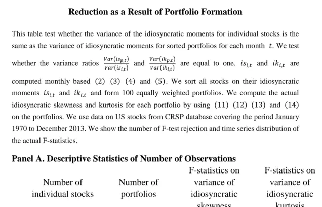
We conduct F-test to test whether portfolios’ actual idiosyncratic moments in our sample have the same variance as individual stocks’ idiosyncratic

(22)

16

moments in our sample. The null hypothesis is that variance of idiosyncratic moments is identical through sorting procedure. At the end of each month, we

test whether variance ratios 𝑉𝑎𝑟(𝑖𝑠_{𝑉𝑎𝑟(𝑖𝑠}𝑝,𝑡)

𝑖,𝑡) and

𝑉𝑎𝑟(𝑖𝑘𝑝,𝑡)

𝑉𝑎𝑟(𝑖𝑘𝑖,𝑡) are equal to one.

where 𝑉𝑎𝑟(𝑖𝑠_𝑖,𝑡) and 𝑉𝑎𝑟(𝑖𝑠_𝑝,𝑡) are the variances of individual stocks’

idiosyncratic skewness and of portfolios’ idiosyncratic skewness in our sample

at the end of month t, respectively; 𝑉𝑎𝑟(𝑖𝑘𝑖,𝑡) and 𝑉𝑎𝑟(𝑖𝑘𝑝,𝑡) are the

variances of individual stocks’ idiosyncratic kurtosis and of portfolios’

idiosyncratic skewness in our sample at the end of month t, respectively.

𝑛_𝑖,𝑡 and 𝑛_𝑝,𝑡 are the numbers of individual stocks and portfolios in month t,

respectively.

3.2.3 Fama-MacBeth Regression at the Individual Stock Level

We conduct Fama-MacBeth regression at the individual stock level following Ang, Hodrick, Xing and Zhang (2009). We run the following

cross-sectional regression at the end of each month t in our sample:

𝑟_𝑖,𝑡+1− 𝑟_𝑓,𝑡+1 = 𝛾_0,𝑡+ 𝛾_1,𝑡𝑖𝑣_𝑖,𝑡+𝛾_2,𝑡𝑖𝑠_𝑖,𝑡+𝛾_3,𝑡𝑖𝑘_𝑖,𝑡+ 𝛾_4,𝑡𝐵𝑒𝑡𝑎_{𝑀𝑎𝑟𝑘𝑒𝑡}_𝑖,𝑡+ 𝛾5,𝑡𝐵𝑒𝑡𝑎_{𝑆𝑀𝐵𝑖,𝑡} + 𝛾6,𝑡𝐵𝑒𝑡𝑎𝐻𝑀𝐿𝑖,𝑡+ 𝛾7,𝑡𝐵𝑒𝑡𝑎𝑈𝑀𝐷𝑖,𝑡+ 𝛾8,𝑡𝐵𝑒𝑡𝑎𝐿𝑖𝑞𝑢𝑑𝑖𝑡𝑦𝑖,𝑡+

𝛾_9,𝑡𝐵𝑒𝑡𝑎_{𝐶𝑜𝑠𝑘𝑒𝑤𝑖,𝑡}+ 𝛾_10,𝑡𝐵𝑒𝑡𝑎_{𝐶𝑜𝑘𝑢𝑟𝑡𝑜𝑖,𝑡}+ 𝛾_11,𝑡𝑚𝑜𝑚_𝑖,𝑡+ 𝛾_12,𝑡𝐵𝑀_𝑖,𝑦 +

𝛾_13,𝑡𝑆𝑖𝑧𝑒_𝑖,𝑦+ 𝜖_𝑖,𝑡 (15)

where 𝑟_𝑖,𝑡+1 and 𝑟_𝑓,𝑡+1are the monthly return for stock i and risk-free rate at

the end of month t+1, respectively;

𝑖𝑣_𝑖,𝑡, 𝑖𝑠_𝑖,𝑡 and 𝑖𝑘_𝑖,𝑡 are idiosyncratic volatility, skewness and kurtosis of

stock i observed in month t, respectively; we estimate all the betas with equation

(10) at the individual stock level; 𝑚𝑜𝑚_𝑖,𝑡 is the cumulative return on stock i

(23)

17

following Fama and French (1992), 𝐵𝑀_𝑖,𝑦 is the book equity over market

equity in December of year y-1 and is identical over year y;

𝑆𝑖𝑧𝑒𝑖,𝑦 is the logarithm of market capitalization of firm i ending in June of year

y and is identical over year y. We then calculate the time-series average of

coefficients ( 𝛾_0,𝑡, 𝛾_1,𝑡, … , 𝛾_13,𝑡), standard error of the coefficients, and t

-statistics. Then, t-statistics can indicate whether idiosyncratic skewness and

(24)

18

Chapter 4. Data Collection

In this Chapter, we describe our individual stock data in section 4.1 and then discuss the market data in section 4.2.

4.1.Description of Individual Stock Data

We use two databases to construct our individual stock dataset. We obtain the holding period return on individual stocks and firm’s market capitalization from CRSP. We also use Compustat to evaluate book equity of individual firms.

4.1.1. Daily Frequency Individual Stock Data

We obtain the return on individual stock from CRSP from January 2, 1970 to December 31, 2013. The dataset also includes ticker, CRSP permanent company number, CUSIP, closing price and share volume. We use the daily holding period return of individual stock to estimate idiosyncratic moments at the end of each month.

The individual stock daily dataset contains 72,242,176 observations, including 28081 firms traded on NYSE, AMEX and NASDAQ stock markets from January 2, 1970 to December 31, 2013. We then remove the empty or non-exist data in the dataset and have 70,755,218 observations left.

Table 1 reports descriptive statistics of numbers of trading companies in each month.

[Please insert Table 1 about here.]

4.1.2. Monthly Frequency Individual Stock Data

We obtain monthly holding period return of individual stock data from CRSP from January 1970 to December 2013. The dataset also includes ticker,

(25)

19

CRSP permanent company number, CUSIP, closing price and share volume. We use monthly return data to estimate the betas in the first step of Fama-MacBeth regression and run the cross-sectional Fama-Fama-MacBeth regressions. Besides, we use the product of closing price and share volume to measure stocks’ market capitalization. We measure firms’ size by the logarithm of market capitalization ending in each June. We use CUSIP to merge CRSP dataset with Compustat dataset.

4.1.3. Annual Frequency Individual Stock Data

We obtain stockholders’ equity, deferred tax liability and investment tax credit from Compustat from the fiscal year of 1969 to 2013. We use the annual frequency data to create book equity of the stock at the end of each fiscal year. Following Fama and French (1992), book equity is equal to stockholders’ equity plus deferred tax liability and investment tax credit (if applicable). Then, the book-to-market ratio is book equity for the fiscal year ending in calendar year

t-1 divided by market equity at the end of December of t-1.

4.2.Description of Market Data

We use CRSP, Kenneth French data library5 and Robert F. Stambaugh

data library6 to get market factors and return on market index.

5_{http://mba.tuck.dartmouth.edu/pages/faculty/ken.french/data_library.html}

6_{http://finance.wharton.upenn.edu/~stambaugh/liq_data_1962_2013.txt, We are thankful that} Dr. Stambaugh made these data available.

(26)

20

4.2.1. Daily Frequency Market Data

We obtain Fama-French three-factor daily dataset from Kenneth French data library; it includes risk free rate, SMB, HML and excess return on the market from January 2, 1970 to December 31, 2013. We use the Fama-French three-factor daily data to compute idiosyncratic moments at the end of each month.

4.2.2. Monthly Frequency Market Data

We obtain monthly risk free rate, SMB factor, HML factor, UMD factor and excess return on the market from Fama-French Factors dataset via Wharton Research Data Services. We use these factors to create factor loadings in

equation (11).

Besides, we obtain monthly liquidity factor from Pastor-Stambaugh data library. We use monthly liquidity factor to get liquidity factor loading in

equation (11).

Finally, to study the correlation between idiosyncratic moments and market return, we obtain value-weighted monthly return and equal-weighted monthly return on CRSP Stock Market Indexes from January 1970 to December 2013.

For the CRSP Stock Market Indexes, the market groups of securities include individual NYSE, AMEX, and NASDAQ markets, as well as the NYSE/AMEX and NYSE/AMEX/NASDAQ market combinations. Published S&P 500 and NASDAQ Composite Index Data are also included.

Besides, we also get the value-weighted monthly return and equal-weighted monthly return on 25 portfolios formed on size and book-to-market ratio from January 1970 to December 2013 via Kenneth French data library.

(27)

21

In addition, we obtain S&P 500 Index monthly returns from CRSP. They are calculated by (SPINDX(t)/SPINDX(t-1)) – 1, where SPINDX is the level of the Standard & Poor's 500 Composite Index (prior to March 1957, 90-stock index) at the end of the month.

(28)

22

Chapter 5. Empirical Findings

In this Chapter, we present our empirical findings. First, in section 5.1, we introduce time series variation of idiosyncratic moments. Second, we discuss the actual idiosyncratic moments of portfolios in section 5.2. Third, we show Fama-MacBeth regressions in section 5.3.

5.1.Time Series Variation of Idiosyncratic Moments

We first study the time series variation of idiosyncratic moments. We use

the methodology described above (equation (3), (4) and (5)) to estimate the

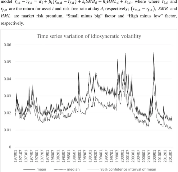
idiosyncratic moments of each stock at the end of each month from January 1970 to December 2013. Then, we get the cross-sectional distribution of idiosyncratic moments in each month. We calculate the mean, median and 95% confidence interval of each distribution. By plotting the statistics, we can show time series variation of idiosyncratic moments. The Figure 1 shows time series variation of idiosyncratic moments.

[Please insert Figure 1 about here.]

Panel A of Figure 1 shows an increasing trend in idiosyncratic volatility from 1977 to 2000, consistent with the findings of Campbell, Lettau, Malkiel and Xu (2001). From panel A, B and C of Figure 1, we suggest that idiosyncratic volatility and idiosyncratic kurtosis are more stable than idiosyncratic skewness over time from 1970 to 2013, consistent with the findings of Harvey and Siddique (1999) and Boyer et al. (2010). Besides, panel B of Figure 1 indicates that idiosyncratic skewness is always positive from 1970 to 2013. This finding is consistent with the finding of Albuquerque (2012). In addition, we find that idiosyncratic volatility reaches its peak during October 1998, December 2000 and October 2008 from panel A of Figure 1. These periods indicate the 1997-1998 Asian financial crisis and 2007-2008 financial crisis. Lastly, we observe

(29)

23

two structural breaks during 1972-1973 and 1992-1993 from panel C of Figure 1.

We describe the descriptive statistics of idiosyncratic moments’ mean and median from January 1970 to December 2013.

In Table 2, from January 1970 to December 2013, mean of idiosyncratic volatility has an average of 0.0270 and a standard deviation of 0.0077; mean of idiosyncratic skewness has an average of 0.1649 and a standard deviation of 0.1211; mean of idiosyncratic kurtosis has an average of 4.0264 and a standard deviation of 0.4452.

Moreover, we also investigate the correlation between idiosyncratic moments and market index returns. We calculate the correlations between equal-weighted idiosyncratic moments (skewness and kurtosis) and CRSP Stock Market Indexes (equal-weighted and value-weighted), 25 portfolios based on size and book-to-market ratio monthly return and S&P 500 index monthly return, separately. Table 3 reports the results.

In Table 3, averaged idiosyncratic skewness is strongly and positively correlated to the three measures of market index returns, with the correlation of 0.5349, 0.7194 and 0.5863, respectively. Averaged idiosyncratic kurtosis is also positively correlated to the three measures of market index returns, with the correlation of 0.0553, 0.0970 and 0.0823, respectively. Correlations between averaged idiosyncratic moments and Fama-French 25 portfolio returns show consistent results. High correlation between averaged idiosyncratic skewness and return of market index indicates that idiosyncratic skewness is a good predictor of stock return realized in the same period.

(30)

24

In addition, we calculate the correlations between idiosyncratic moments

and market factors. We include all the market factors in equation (11).

Equal-weighted idiosyncratic moments are created at the end of each month from January 1970 to December 2013. All the factors are on a monthly basis from January 1970 to December 2013. We show results in Table 4.

In Table 4, we find that correlations between idiosyncratic skewness and other factors or idiosyncratic moments are all significant at 5% level except for liquidity factor. Idiosyncratic skewness is highly correlated with SMB (with the correlation 0.476, significant at 1% level) and market risk premium (with the correlation 0.577, significant at 1% level). High and significant correlations between idiosyncratic skewness and other factors indicate that pricing capability of idiosyncratic skewness could be attributed SMB factor and market risk premium factor. We find that idiosyncratic kurtosis and idiosyncratic volatility share a correlation of -0.265, significant at 1% level.

5.2. Actual Idiosyncratic Moments of Portfolios

We estimate the actual idiosyncratic moments of portfolios. At the end of

each month t from January 1970 to December 2013, we sort stocks into ten

portfolios ranking on their idiosyncratic skewness or idiosyncratic kurtosis

observed at the end of month t. We compute daily equal-weighted returns for

the portfolio and use Fama-French three factor model to estimate the

distribution of residuals in month t. Then, we estimate the idiosyncratic

moments of portfolio in month t using equation (12), (13) and (14). In Table

5, we report descriptive statistics of portfolios’ actual idiosyncratic moments. [Please insert Table 5 about here.]

(31)

25

Column 3, 4, 5 and 6 in Table 5 show that idiosyncratic moments of portfolio shrink to a lower range. Besides, we find that the average one-period forward returns for the lowest idiosyncratic volatility decile exceed the ones of the highest idiosyncratic volatility decile by 0.61% per month; average one-period forward returns for the highest idiosyncratic skewness decile exceed the ones of the lowest idiosyncratic skewness decile by 0.08% per month; the average one-period forward returns for the highest idiosyncratic kurtosis decile exceed the ones of the lowest idiosyncratic kurtosis decile by 0.07% per month. We do not observe any monotonic trends among expected returns in different deciles. In panel C of Table 5, column (4) and column (6) show that averaged and actual idiosyncratic kurtosis of the portfolio have different monotones, suggesting that actual idiosyncratic kurtosis of the portfolio is not a linear combination of their individual level counterpart.

We conduct an F-test to test whether actual idiosyncratic moments of portfolios have the same variance as that of the idiosyncratic moments of individual stocks. The null hypothesis is that variance of idiosyncratic moments stay constant after sorting procedure. We include one hundred portfolios formed through ranking idiosyncratic moments sorting as mentioned in section 3.2.1 in our F-test. We present our results in Table 6.

Panel B of Table 6 reports the results of F-tests. We run our F-test at the end of each month from January 1970 to December 2013. We reject 523 out of 528 tests in idiosyncratic skewness sorting procedure and reject 525 out of 528 tests in idiosyncratic kurtosis sorting procedure at 5% significance level. These results indicate that actual idiosyncratic moments of portfolios and of individual stocks come from different distributions. We suggest that diversification effects

(32)

26

in the sorting procedure change the actual idiosyncratic moments’ distribution of portfolios.

5.3.Fama-MacBeth Regressions

5.3.1 Fama-MacBeth Regression at the individual level

To assess the pricing effects of idiosyncratic skewness and kurtosis, we conduct cross-sectional regressions approach following Fama and MacBeth (1973). We find a negative and significant relationship between idiosyncratic skewness and expected returns in cross-section, consistent with Boyer et. al (2010). In our model, we includes idiosyncratic skewness and kurtosis, along

with other market factors loadings and characteristics shown in equation(15).

Table 7 reports our results.

We include all betas and characteristics in cross-sectional regressions and

report the average of coefficients and t-statistics in Column 3 of Table 7.

Besides, we just include characteristics in cross-sectional regressions and report the results in Column 2 of Table 7. Column 1 of Table 7 only includes factor loadings and idiosyncratic moments as explanatory variables.

Table 7 indicates that whether we include the factor loadings only (column 1), the characteristics only (column 2), or both factor loadings and characteristics (column 3), the coefficients on idiosyncratic skewness are negative and significant at 1% level, with the value of 0.1%, 0.11% and -0.12%, respectively. The results indicate that pricing effect of idiosyncratic skewness is robustness to the different factors and characteristics usually included in the Fama-MacBeth pricing tests. We show that idiosyncratic

(33)

27

skewness can contribute to explaining the one-month forward expected return. In column 1 of table 7, risk premium on HML factor is positive and significant at 5% level; risk premiums on UMD factor and coskewness are negative and significant at 1% level. Column 2 and column 3 show that size and momentum can also help explain the expected return. Idiosyncratic volatility and skewness are not priced in the model.

In Figure 2, we plot the time series of coefficients on 𝑖𝑠_𝑖,𝑡 and 𝑖𝑘_𝑖,𝑡 in

Column 3 of Table 7.

[Please insert Figure 2 about here.]

Panel A of Figure 2 indicates that the coefficient on idiosyncratic skewness reaches its maximum level at 2.28% in November 1999. It also indicates that the coefficient on idiosyncratic skewness reaches its minimum level at -2.44% in January 1975. Panel B of Figure 2 indicates that the coefficient on idiosyncratic kurtosis reaches its maximum level at 0.77% in September 1978. It also indicates that the coefficient on idiosyncratic kurtosis reaches its minimum level at -1.57% in January 2000.

5.3.2 Tests on Sub-period Samples at the Individual Level

We create period samples and run Fama-MacBeth regressions on sub-period datasets. We run this sub-sub-period sample test for several reasons. First, we observe two noticeable structural breaks in averaged idiosyncratic kurtosis in panel C of Figure 1. Second, we find that idiosyncratic volatility increases from the lowest level to the highest level during the financial crisis from 2007-2008 in panel A of Figure 1. We can investigate the impact of financial crisis on idiosyncratic moments pricing effect by testing whether our model is

(34)

28

predicable during financial crisis. Moreover, we can assess the stability of the skewness pricing results.

We first split our sample using endogenously determined structural breaks7_.

We create breakpoints at April 1992 and June 2007. Specifically, April 1992 is one of the structural break dates shown in panel C of Figure 1 (The other structural break point at 1972 is ignored because the data is not included in Fama-MacBeth cross-sectional regression). Besides, June 2007 is the beginning date of financial crisis. Table 8 presents our sub-period tests results.

The results in sub-period samples tests are consistent with the ones in the overall sample test. Specifically, in Table 8, we find that in the sub-period of January 1975-April 1992 and July 2007-November 2013, idiosyncratic skewness shows pricing capability at 1% and 5% significant level, respectively. The pricing effect of idiosyncratic skewness disappears during May 1992 to June 2007. In the same period, coefficients on idiosyncratic volatility and kurtosis are 14.9% and -0.06%, respectively, both significant at 1% level. In the other two sub-periods (January 1975-April 1992 and July 2007-November 2013), coefficients on idiosyncratic volatility are negative, consistent with Ang et. al (2006). Besides, we find that only idiosyncratic skewness can help explain expected return during the period July 2007-November 2013 in our model, indicating that idiosyncratic skewness is a strong predictor of expected return during the financial crisis period. The results in the July 2007-November 2013 show that our model is predictable during the financial crisis period.

7_{Following Bai and Perron (2003), we employ the multiple structural change test to test the} structural breakpoint in the time series of idiosyncratic moments. We do find two structural breaks that correspond to the two structural breakpoints observed in Panel C of Figure 1 (in 1972 and 1992). We do not find any structural breaks in the time series of idiosyncratic volatility or skewness.

(35)

29

Besides, we divide our sample into three equal sub-periods. Table 9 presents our equal-sized sub-period tests

In Table 9, at the first and second sub-period, coefficients on idiosyncratic skewness are -0.17% and -0.13%, respectively, significant at 1% level. Besides, we find that coefficients on idiosyncratic skewness have an increasing trend over time, with the value -0.17%, -0.13% and -0.06% in three equal-sized sub-period, respectively. Table 8 and Table 9 show consistent results, indicating that the idiosyncratic skewness pricing results at the individual level is robustness. We also find that idiosyncratic volatility is positive related to expected returns in the period December 1987 to November 2001, consistent with the sub-period test created on structural break. Moreover, Table 9 shows that idiosyncratic kurtosis is irrelevant to explaining the expected return.

5.3.3 Fama-MacBeth Regression at the Portfolio Level

In this section, we discuss Fama-MacBeth regression at the portfolio level as an alternative approach. We use the cross-sectional regression outlined as

equation(15). Table 10 reports the testing results on portfolios sorted on

ranking idiosyncratic skewness.

Table 10 shows some evidence that idiosyncratic skewness is priced. Specifically, in column 2 of Panel A, the coefficient on idiosyncratic skewness is -0.06%, significant at 5% level. In column (1) and (3) of Table 10, we find that pricing effect of idiosyncratic skewness disappears when we include factor loadings in our model. One possible explanation for this contradiction is factor loadings are correlated to the idiosyncratic moments. We also show that SMB

(36)

30

and UMD factor can attribute to explaining the expected return. Moreover, we find that idiosyncratic volatility and kurtosis are not priced.

We find a negative and significant pricing effect of idiosyncratic skewness when testing idiosyncratic kurtosis-sorted portfolios, consistent with our main finding. Table 11 reports the testing results on portfolios sorted on ranking idiosyncratic kurtosis.

Table 11 indicates that the coefficients on idiosyncratic skewness in idiosyncratic kurtosis-sorted procedure are negative and significant at 1% level, with the value -0.23%, -0.24% and -0.26%. Besides, idiosyncratic volatility and idiosyncratic kurtosis are not priced, consistent with the results in individual stock level tests. Risk premiums of HML are positive and significant at 5% level in both sorting procedures. Moreover, momentum can help explain portfolio expected returns in kurtosis-sorted procedure.

In Figure 3, we plot the time series of coefficients on 𝑖𝑠_𝑖,𝑡 and 𝑖𝑘_𝑖,𝑡 in

Column 3 of Table 10. In Figure 4, we plot the time series of coefficients on

𝑖𝑠𝑖,𝑡 and 𝑖𝑘𝑖,𝑡 in Column 3 of Table 11.

[Please insert Figure 3 about here.] [Please insert Figure 4 about here.]

Our research on Fama-MacBeth regression at the portfolio level supports our finding: idiosyncratic skewness has additional contribution in explaining the cross-section of expected returns while idiosyncratic volatility and kurtosis are not priced. We show that idiosyncratic skewness is not priced when portfolios are formed through idiosyncratic skewness sorting, while it is priced when portfolios are formed through idiosyncratic kurtosis sorting.

(37)

31

5.3.4 Tests on Sub-period Samples at the Portfolio Level

We conduct sub-period sample tests at the portfolio level. The sub-period samples are created on structural break or equally created, same as the approaches in 5.3.2. Our object is to assess the stability of the skewness pricing results in Fama-MacBeth approach at the portfolio level. Table 12 and Table 13 report sub-period tests on Fama-MacBeth regression at the portfolio level sorted on idiosyncratic skewness.

[Please insert Table 12 about here.] [Please insert Table 13 about here.]

Results in Table 12 are consistent with former results in the overall dataset in section 5.3.3. Specifically, idiosyncratic volatility, skewness and kurtosis show no pricing effects in the three equal-sized sub-periods. In Table 13, idiosyncratic volatility shows negative pricing effects in the sub-period from January 1975 to November 1987, consistent with the finding of Ang et al. (2006). Neither idiosyncratic skewness nor idiosyncratic kurtosis is priced in the sub-period test created on structural break.

Table 14 and Table 15 report sub-period tests on Fama-MacBeth regression at the portfolio level sorted on idiosyncratic kurtosis.

[Please insert Table 14 about here.] [Please insert Table 15 about here.]

We can find some evidence that idiosyncratic skewness is priced when testing the idiosyncratic kurtosis-sorted portfolios. In Table 14, coefficient on idiosyncratic skewness in the first sub-period is -0.0023, significant at 1% level. In Table 15, coefficients on idiosyncratic skewness are negative and significant at 10% level in the first and third sub-period. We also find that idiosyncratic

(38)

32

volatility is positive and significant related to expected return from May 1992 to June 2007 in Table 14 and from December 1987 to November 2011 in Table 15. Idiosyncratic kurtosis is not priced in each sub-period, consistent with our main results.

(39)

33

Chapter 6. Conclusion

Previous research have studied the pricing effects of idiosyncratic volatility and skewness. Ang, Hodrick, Xing and Zhang (2006) find that idiosyncratic volatility is negatively related to the return on the market. Boyer, Mitton and Vorkink (2010) suggest that expected idiosyncratic skewness is negatively related to expected return. However, to our knowledge, literature does not shed light on the pricing effect of idiosyncratic kurtosis. Time series variation and pricing effect of idiosyncratic kurtosis remain unknown. Our study addresses these issues by investigating the time series variation of average idiosyncratic skewness and kurtosis, as well as pricing effects of idiosyncratic higher moments (volatility skewness and kurtosis) using the Fama-MacBeth approach.

Our idiosyncratic moments’ estimations follows Boyer, Mitton and Vorkink (2010). We regress the daily returns of each stock on daily SMB, HML and market risk premium factor at the end of each month. We then get the residuals of the Fama-French three factor model and estimate the moments of residuals. Moments of residuals are the idiosyncratic moments of the stock.

We study the time series variation of idiosyncratic moments from 1970 to 2013. We suggest that idiosyncratic volatility and idiosyncratic kurtosis are more stable than idiosyncratic skewness. Besides, we observe two structural breaks in time series variation of idiosyncratic kurtosis and find that idiosyncratic volatility reaches its peak during financial crisis from 2007 to 2008.

We estimate the actual idiosyncratic moments of portfolios. We present that actual idiosyncratic kurtosis of portfolios formed through ranking idiosyncratic kurtosis sorting is not a monotonic sequence. We also show that

(40)

34

actual idiosyncratic moments of portfolios and of individual stocks come from different distributions.

Using a sample of US stocks traded on NYSE, AMEX and NASDAQ stock markets from January 1970 to December 2013, we find that coefficient on idiosyncratic skewness in the Fama-MacBeth regression at the individual stock level is negative and significant at 5% level, consistent with the finding of Boyer et al. (2010). We also run sub-period sample tests to test the robustness. We create the breakpoints of the sample based on the date of structural break observed in time series variation of idiosyncratic kurtosis and beginning date of financial crisis. The results of the test on sub-period samples are consistent with the ones of the test on whole sample. Besides, we find that idiosyncratic skewness is a strong predictor of expected return in financial crisis period.

We also take typical Fama-MacBeth regression at the portfolio level. We find that idiosyncratic skewness is priced testing on idiosyncratic kurtosis-sorted portfolio. The results of sub-period test at the portfolio level support our main finding that idiosyncratic skewness has negative pricing effect while idiosyncratic volatility and kurtosis is not priced.

Our research contributes to the literature in the following areas: (1) we study the time series variation of idiosyncratic kurtosis and identify two structural breaks in 1972-1973 and 1992-1993. (2) We estimate the actual idiosyncratic moments of the portfolios. We show that actual idiosyncratic kurtosis of portfolios formed through ranking idiosyncratic kurtosis sorting is not a monotonic sequence. (3) By conducting Fama-MacBeth regression at the individual level, we confirm the main result of Boyer et al. (2010) that idiosyncratic skewness has negative pricing effects. We find some consistent results when testing on sub-period samples. Idiosyncratic skewness is not priced when portfolios are formed through idiosyncratic skewness sorting, while it is

(41)

35

priced when portfolios are formed through idiosyncratic kurtosis sorting. We also shed light on the pricing effect of idiosyncratic kurtosis. We conclude that idiosyncratic kurtosis is not priced.

Our research of idiosyncratic moments pricing effects can be extended in several ways. First, more light could be shed on investigating the cause of the structural break in idiosyncratic kurtosis during 1972-1973 and 1992-1993. Second, further research could focus on the period after financial crisis to fully explain why only idiosyncratic skewness shows pricing ability in the period. Last, we find that idiosyncratic skewness is not priced when portfolios are sorted through idiosyncratic skewness ranking, while it is priced at the individual stock level or portfolio sorted through idiosyncratic kurtosis ranking. Further investigation is required to explaining this puzzling finding.

(42)

36

Reference

Albuquerque, R. (2012). Skewness in stock returns: reconciling the

evidence on firm versus aggregate returns. Review of Financial Studies,

25(5), 1630-1673.

Ang, A., Hodrick, R. J., Xing, Y., & Zhang, X. (2006). The cross‐

section of volatility and expected returns. The Journal of Finance, 61(1),

259-299.

Ang, A., Hodrick, R. J., Xing, Y., & Zhang, X. (2009). High idiosyncratic volatility and low returns: International and further US

evidence. Journal of Financial Economics, 91(1), 1-23.

Bai, J., & Perron, P. (2003). Critical values for multiple structural

change tests. The Econometrics Journal, 6(1), 72-78.

Barberis, N., & Huang, M. (2008). Stocks as Lotteries: The

Implications of Probability Weighting for Security Prices. The

American Economic Review, 98(5), 2066-2100.

Black, F., M.C. Jensen & M., Scholes. (1972). The Capital Asset Pricing Model: Some Empirical Tests, in Studies in the Theory of Capital Markets. Michael C. Jensen, ed. New York: Praeger, 79-121.

Boyer, B., Mitton, T., & Vorkink, K. (2010). Expected

idiosyncratic skewness. Review of Financial Studies, 23(1), 169-202.

Campbell, J. Y., Lettau, M., Malkiel, B. G., & Xu, Y. (2001). Have individual stocks become more volatile? An empirical exploration of

idiosyncratic risk. The Journal of Finance, 56(1), 1-43.

Chang, B. Y., Christoffersen, P., & Jacobs, K. (2013). Market

skewness risk and the cross section of stock returns. Journal of

Financial Economics, 107(1), 46-68.

Christie-David, R., & Chaudhry, M. (2001). Coskewness and

(43)

55-37

81.

Douglas, G. W. (1967). Risk in the equity markets: An empirical

appraisal of market efficiency (Doctoral dissertation, Yale University.).

Fama, E. F., & French, K. R. (1992). The cross‐ section of

expected stock returns. The Journal of Finance, 47(2), 427-465.

Fama, E., & French,K., (1993). Common risk factors in the returns

on stocks and bonds. Journal of Financial Economics 33, 3–56

Fama, E. F., & MacBeth, J. D. (1973). Risk, return, and equilibrium:

Empirical tests. The Journal of Political Economy, 607-636.

Fang, H., & Lai, T. Y. (1997). Co‐kurtosis and Capital Asset

Pricing. Financial Review, 32(2), 293-307.

Friend, I., & Blume, M. (1970). Measurement of portfolio

performance under uncertainty. The American Economic Review,

561-575.

Friend, I., & Westerfield, R. (1980). Co‐skewness and capital asset

pricing. The Journal of Finance, 35(4), 897-913.

Fu, F. (2009). Idiosyncratic risk and the cross-section of expected

stock returns. Journal of Financial Economics, 91(1), 24-37.

Goyal, A., & Santa‐Clara, P. (2003). Idiosyncratic risk matters! The

Journal of Finance, 58(3), 975-1008.

Guidolin, M., & Timmermann, A. (2008). International asset allocation under regime switching, skew, and kurtosis preferences.

Review of Financial Studies, 21(2), 889-935.

Guo, H., & Savickas, R. (2010). Relation between time-series and cross-sectional effects of idiosyncratic variance on stock returns.

Journal of Banking & Finance, 34(7), 1637-1649.

Harvey, C. R., & Siddique, A. (1999). Autoregressive conditional

Are Idiosyncratic Skewness and Idiosyncratic Kurtosis Priced?