Sensitivity of Direct Runoff to Curve Number Using the SCS-CN Method

(1)

Civil Engineering Journal

Vol. 5, No. 12, December, 2019

Sensitivity of Direct Runoff to Curve Number Using the

SCS-CN Method

AG Soomro

a, b*

_{, MM Babar}

a

_{, A Memon}

a, b

_{, A. Z. Zaidi}

a

_{, A Ashraf}

b

_{, J. Lund}

c a _{US Pakistan Center for Advanced Studies in Water, Mehran University of Engineering and Technology, Jamshoro, Pakistan.}

b _{Pakistan Agricultural Research Council.}

c _{Department of Geography, The University of Utah, Utah, United States.} Received 27 June 2019; Accepted 18 October 2019

Abstract

This study explores the impact of runoff curve number (CN) on the hydrological model outputs for the Morai watershed, Sindh-Pakistan, using the Soil Conservation Service Curve Number (SCS-CN) method. The SCS-CN method is an empirical technique used to estimate rainfall-runoff volume from precipitation in small watersheds, and CN is an empirically derived parameter used to calculate direct runoff from a rainfall event. CN depends on soil type, its condition, and the land use and land cover (LULC) of an area. Precise knowledge of these factors was not available for the study area, and therefore, a range of values was selected to analyze the sensitivity of the model to the changing CN values. Sensitivity analysis involves a methodological manipulation of model parameters to understand their impacts on model outputs. A range of CN values from 40-90 was selected to determine their effects on model results at the sub-catchment level during the historic flood year of 2010. The model simulated 362 cumecs of peakdischarge for CN=90; however, for CN=40, the discharge reduced substantially to 78 cumecs (a 78.46% reduction). Event-based comparison of water volumes for different groups of CN values—90-75, 80-75, 75-70, and 90-40 —showed reductions in water availability of 8.88%, 3.39%, 3.82%, and 41.81%, respectively. Although it is known that the higher the CN, the greater the discharge from direct runoff and the less initial losses, the sensitivity analysis quantifies that impact and determines the amount of associated discharges with changing CN values. The results of the case study suggest that CN is one of the most influential parameters in the simulation of direct runoff. Knowledge of accurate runoff is important in both wet (flood management) and dry periods (water availability). A wide range in the resulting water discharges highlights the importance of precise CN selection. Sensitivity analysis is an essential facet of establishing hydrological models in limited data watersheds. The range of CNs demonstrates an enormous quantitative consequence on direct runoff, the exactness of which is necessary for effective water resource planning and management. The method itself is not novel, but the way it is proposed here can justify investments in determining the accurate CN before initiating mega projects involving rainfall-runoff simulations. Even a small error in CN value may lead to serious consequences. In the current study, the sensitivity analysis challenges the strength of the results of a model in the presence of ambiguity regarding CN value.

Keywords: SCS-CN Method; Initial Abstraction; Direct Runoff; HEC-HMS; Hydrological Model; Sensitivity Analysis.

1. Introduction

A thorough assessment of the hydrologic response of a watershed is essential for water resource planning and management at the watershed level. Models are the abstraction of real phenomena based on many assumptions. These assumptions are acceptable as far as they do not produce erroneous results. The accuracy of the assessment depends on

* Corresponding author: [email protected] http://dx.doi.org/10.28991/cej-2019-03091445

© 2019 by the authors. Licensee C.E.J, Tehran, Iran. This article is an open access article distributed under the terms and conditions of the Creative Commons Attribution (CC-BY) license (http://creativecommons.org/licenses/by/4.0/).

(2)

the proper choice of methods and procedures, the correctness of the input parameters, and the feasibility of the assumptions used. An accurate assessment will yield reliable discharges that may decrease risks of water-related hazards such as flood damages and water shortages.

In the mid-1930s, the US Soil Conservation Service (SCS) (now known as the Natural Resources Conservation Service) perceived an acute need for hydrologic data for the design of conservation practices. Owing to the intricacy of hydrologic systems and the inaccessibility of pertinent watershed data, the SCS developed the SCS-CN method to estimate rainfall-runoff or immediate water availability. The SCS-CN method is the function of the amount of precipitation, basin slope, soil type/condition, and land use and land cover [1]. It is a simple method intended to be easily accessible and adaptable for ungauged catchments.

The SCS conducted initial experiments, hiring three scientists: W.W. Homer, R.E. Horton, and R.K. Sherman. Horton (1933) worked on the model, categorizing infiltration capacity curves for initial abstraction and excess runoff [2], and Homer (1940) concentrated on the infiltration capacity (initial abstraction) of small watershed data [3]. In early 1940, the rainfall-runoff method was developed by Horner using field-collected infiltration data to simulate runoff volume. This method provided the basis for the SCS-CN technique, established in 1954. The SCS-CN method is the outcome of precise field observations from the late 1930s and early 1940s, followed by numerous scientific experiments. The work of Mockus, Sherman, Andrews, and Ogrosky recognized in the National Engineering Handbook (NEH-4) issued by the SCS in 1956, U.S. Department of Agriculture (USDA) [4-7]. Model improvements and revisions made in 1964, 1965, 1971, 1972, 1985, and 1993. The methods specified by Mockus and Andrews [4, 6] were interpreted by Cowan [8] to produce the present SCS-CN technique based on the water balance equation.

The Hydrologic Engineering Center’s Hydrologic Modeling System (HEC-HMS) includes the SCS-CN loss method to study the effects of a rainfall event in a watershed. In the HEC-HMS model, interception, evaporation, and infiltration processes are loss elements, and they are calculated using transform components [9]. The HEC-HMS model has been used successfully to estimate rainfall-runoff in small watersheds throughout the world (Razi et al. [10]. Knebl et al. (2005) assessed several hydrological models to predict flooding on a regional level and found the HEC-HMS model capable of simulating rainfall-runoff for different features of the watershed area [11]. Yener et al. (2006) successfully employed the HEC-HMS in the Yuvacik Basin of Turkey using occasion-based hourly data and intensity-duration-frequency (IDF) curves to derive rainfall-runoff scenarios [12]. Shieh et al. (2007) used the HEC-HMS model in Taiwan to estimate the impact of check-dams on river discharge with satisfactory results [13]. Zorkeflee et al. (2009) researched the Sungai Kurau Basin for catchment management using GIS and the HEC-HMS model, revealing that the hydrologic behavior varies according to land use [14]. Verma et al. (2010) examined HEC-HMS and Water Erosion Prediction Project (WEPP) models to estimate rainfall-runoff in the Baitarani catchment of India and defended the suitability of the HEC-HMS model for this purpose [15]. Dastoran et al. (2011) determined the ability of HEC-HMS to simulate rainfall-runoff and observed that CN and initial loss are the most significant parameters affecting the results [16].

The above review was undertaken regionally to predict flood waves in the absence of precise CN values. This study employs the SCS-CN method in the HEC-HMS using measured precipitation data and evaluates the SCS-CN estimates for changing CNs through sensitivity analysis. The sensitivity analysis improves the confidence level and evaluates the effectiveness of a modeling approach and is also a major cause of success [17]. Hawkins et al. [18] contribute a hydrological database that proves that the Sensitivity (λ) and SCS-CN are used frequently in model designs. It has become known that the existing approaches for SCS-CN are overdesigned [19]. Tassew et al. [17] simulated flows using the hydrologic modeling approach of the HEC-HMS in Lake, Ethiopia. For the study purpose, they selected a catchment of 1609 km2_{, ran the model, and projected runoff by accounting the losses and flow routing, employing SCS-CN.} Initially, their results showed variability between the observed and the simulated peak flows. Finally, their sensitivity analysis showed that the CN played a sensitive role in the simulation of flows [18].

Many variables are used in rainfall-runoff estimations, and using hydrologic models to speculate the frequency of flood incidents adequately is always a challenging task where there is changing land use, land cover, and climate scenarios [12,19,20,21]. Selecting an appropriate CN is necessary for producing consistent results. CN values based on the watershed characteristics—land use (treatment), land cover (vegetation), soil (type and antecedent moisture situations) [22]. Experimental results show that many important decisions and expectations are made based on hydrologic modeling results, which are employed differently for each location. Appropriate parametric selection is thus essential for sustainable and realistic water resource management. Sensitivity analysis is an integral part of model development and involves an analytical examination of input parameters to aid in model validation and to guide future research.

In this study, we perform a sensitivity analysis to evaluate the impact of CN on direct runoff. We use the HEC-HMS hydrological model to develop a relationship between rainfall-runoff and CN for future water resource planning and development in the study area. The novelty of the study lies in the proposed methodology—the use of sensitivity analysis in regions with limited data and budgets to assess the necessity of additional investments for determining accurate CN values. If model results are not sensitive to CN, then there is no need to determine precise CN values. However, when

(3)

results are highly sensitive, then even a small error in CN value may have severe consequences.

2. Material and Methods

2.1. Study Area

This study designed for the Morai ungauged watershed, which spreads over 492.6 km2_{in the Kohistan, Khirthar} mountain range of Sindh province, Pakistan (Figure 1). The watershed is located in an arid to semi-arid climate. The study area has numerous basins and sub-basins that rely on precipitation for water availability, as no irrigation infrastructure is in place due to its high altitude. The Kohistan region has experienced several devastating floods and droughts in the past 81 years (1933-2013). Droughts and flash floods have been prevalent in recent decades. The latest drought (1996-2002) harshly struck the study area, reducing water resources, agricultural productivity, groundwater levels, and water quality and increasing livestock deaths, mortality rates, migration rates, and poverty [23]. A historic flood took place in 2010, which resulted in human lives lost, destruction of properties and infrastructure, elimination of agricultural assets, breached field embankments, and damaged dug wells.

Figure 1. Layout map of Morai watershed

2.2. Data

The Water and Power Development Authority (WAPDA) of Pakistan provided precipitation data for the region from 1933-2013 from which the data for the flood year 2010 were used to achieve the study goals. The Advanced Land Observing Satellite’s (ALOS) Digital Elevation Model (DEM) at 30m resolution acquired through the US Geological Survey website. The United States-Pakistan Center for Advanced Studies (USPCAS-W) of Mehran University of Engineering and Technology, Jamshoro facilitated the use of Geographical Information System software (ArcGIS version 10.3.1).

2.3. Hydrologic Software

We conducted the rainfall-runoff modeling for the Thana Boula Khan (TBK) catchment using the HEC-HMS model and its GIS extension, HEC-GeoHMS. We brought the ALOS DEM into the ArcGIS interface (HEC-GeoHMS) to integrate spatial and hydrological parameters and to set up the basin’s physiographic database for the hydrologic model [24]. We employed the HEC-HMS model to simulate the initial abstraction and direct runoff, and we did not count the base-flow due to the selection of a precipitation-based flood event in the watershed. We used the Loss Model to estimate the runoff volume by calculating the losses due to initial abstraction, percolation, storage, and evaporation, deducting them from the precipitation. We used the Transform Model to reproduce the direct runoff through additional rainfall over the watershed, which required only lag time. We used the Muskingum Routing Model to model flood wave through the channel and produce flood hydrographs [25]. McCarthy [26] established a Muskingum method in 1938, which is the lumped flow routing technique we used in the current sensitivity analysis.

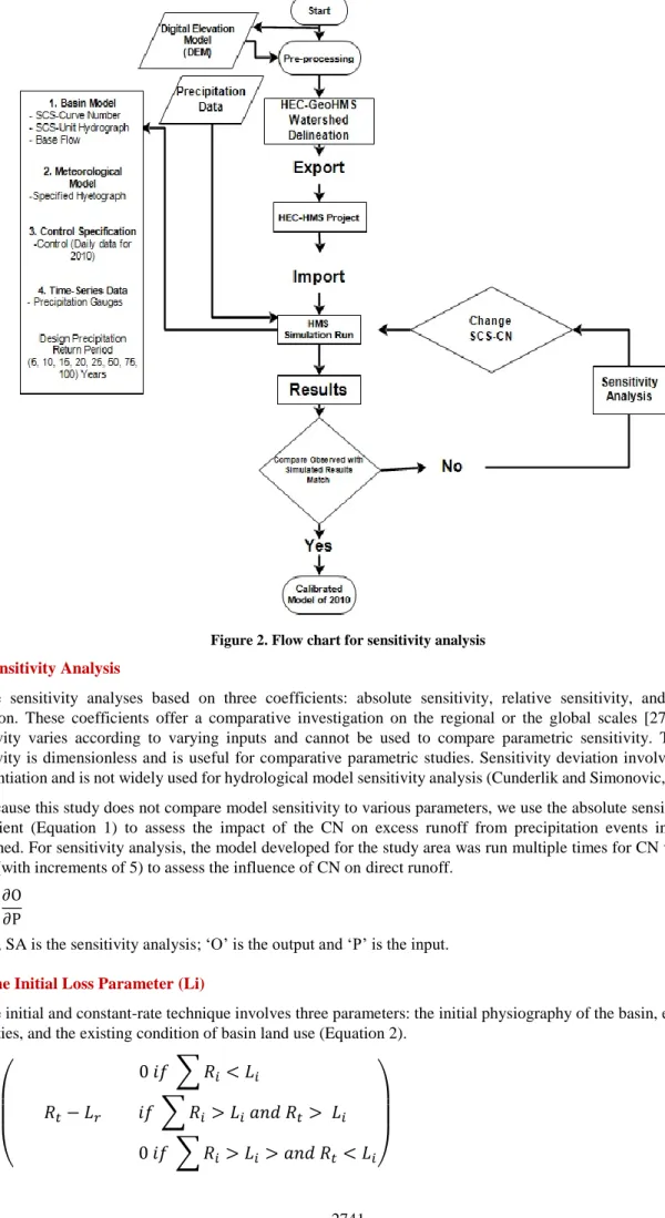
We used the default SCS-CN in HEC-HMS to simulate water availability through rainfall-runoff processes in the study area. In the HEC-HMS model, each parameter describes specific hydrologic conditions. We selected the CN that characterizes infiltration and interception for the sensitivity analysis. We detail the methodology in the flow chart (Figure 2).

(4)

Figure 2. Flow chart for sensitivity analysis

2.4. Sensitivity Analysis

The sensitivity analyses based on three coefficients: absolute sensitivity, relative sensitivity, and sensitivity deviation. These coefficients offer a comparative investigation on the regional or the global scales [27]. Absolute sensitivity varies according to varying inputs and cannot be used to compare parametric sensitivity. The relative sensitivity is dimensionless and is useful for comparative parametric studies. Sensitivity deviation involves complex differentiation and is not widely used for hydrological model sensitivity analysis (Cunderlik and Simonovic, 2004) [28].

Because this study does not compare model sensitivity to various parameters, we use the absolute sensitivity troika coefficient (Equation 1) to assess the impact of the CN on excess runoff from precipitation events in the Morai watershed. For sensitivity analysis, the model developed for the study area was run multiple times for CN values from 40-90 (with increments of 5) to assess the influence of CN on direct runoff.

SA =∂O

∂P (1)

Where; SA is the sensitivity analysis; ‘O’ is the output and ‘P’ is the input. 2.5. The Initial Loss Parameter (Li)

The initial and constant-rate technique involves three parameters: the initial physiography of the basin, existing soil properties, and the existing condition of basin land use (Equation 2).

𝑅

_𝑒𝑡=

(

0 𝑖𝑓 ∑ 𝑅

𝑖

< 𝐿

_𝑡−1 (3)

Where It is the average inflow to storage at time t, and CA and CB are routing coefficients given by:

𝐶𝐴=_{𝑆𝑡 + 0.5𝛥}𝛥𝑡 𝑎𝑛𝑑 𝐶𝐵 = 1 − 𝐶𝐴 (4)

Where; Δt represents the computational time stage.

3. Results and Discussions

The sensitivity procedure described in the previous section has been applied to the Morai watershed using precipitation data of the year 2010—a historical flood year in Pakistan. The CNs have been assessed, ranging from 40-90, for their impact on initial loss and direct runoff. The changing CN displayed a dynamic effect on the outputs. The results are discussed in detail here.

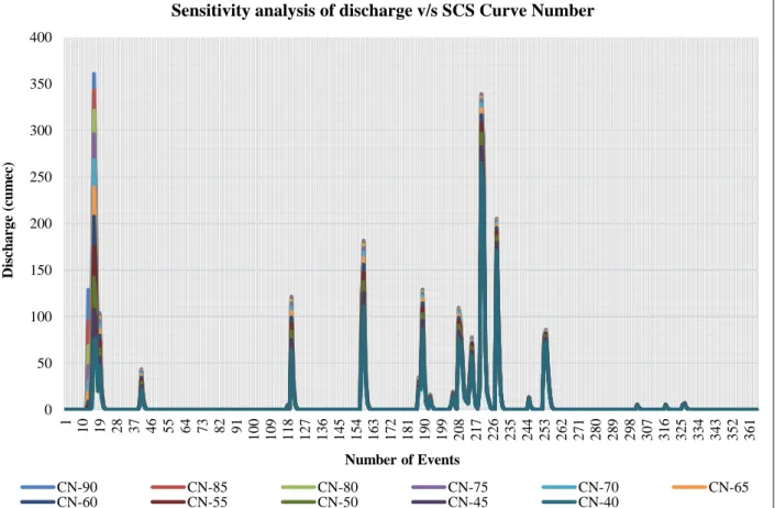
Figure 3. Curve numbers and their associated discharges

Figure 3 shows direct runoff for the event-based HEC-HMS model run for varying CNs for the 2010 flood event. It is known that direct runoff increases with the increase in CNs, but how much it changes is being ascertained in this study. The results depict that the maximum discharge of 362 cumecs was simulated using CN 90, while CN 40 produced a discharge of 78 cumecs keeping all other model parameters unchanged.

0 50 100 150 200 250 300 350 400 1 10 19 28 37 46 55 64 73 82 91 1 0 0 1 0 9 1 1 8 1 2 7 1 3 6 1 4 5 1 5 4 1 6 3 1 7 2 1 8 1 1 9 0 1 9 9 2 0 8 2 1 7 2 2 6 2 3 5 2 4 4 2 5 3 2 6 2 2 7 1 2 8 0 2 8 9 2 9 8 3 0 7 3 1 6 3 2 5 3 3 4 3 4 3 3 5 2 3 6 1 Disc h a rg e (c u m ec ) Number of Events

Sensitivity analysis of discharge v/s SCS Curve Number

CN-90 CN-85 CN-80 CN-75 CN-70 CN-65

(6)

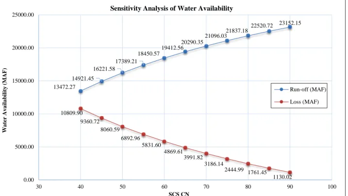
Figure 4. Sensitivity analysis of water availability

Figure 4 portrays the comparative analysis of initial abstraction and direct runoff in Million Acre Feet (MAF) by using CN values (40-90 with an increment of 5). Eleven CN values from 40-90 were used to simulate direct runoff. The results revealed that CN 40 generated 10,809.90 MAF of initial abstraction and produced 13,472.27 MAF of direct runoff. However, CN 90 simulated 1130.02 MAF of initial abstraction and 23,152.15 MAF of direct runoff.

Figure 5. Selection of SCS-CN and variation of water availability

Figure 5 illustrates the percent-wise variation of water availability using different CN values. Four groups with different CN ranges were selected to determine the range of simulated direct runoff within these groups. We tested the

8.88 3.39 3.82 41.81 0.00 5.00 10.00 15.00 20.00 25.00 30.00 35.00 40.00 45.00 90-75 80-75 75-70 90-40 V a ria tio n in W a te r Av a il a b il ity (% ) SCS CN

Selection of SCS CN and variation of Water Availability (%)

23152.15 22520.72 21837.18 21096.03 20290.35 19412.56 18450.57 17389.21 16221.58 14921.45 13472.27 1130.02 1761.45 2444.99 3186.14 3991.82 4869.61 5831.60 6892.96 8060.59 9360.72 10809.90 0.00 5000.00 10000.00 15000.00 20000.00 25000.00 30 40 50 60 70 80 90 100 W a te r A v a il a b il it y ( M A F) SCS CN

Sensitivity Analysis of Water Availability

Run-off (MAF) Loss (MAF)

(7)

CN groups with ranges 90-75, 80-75, 75-70, and 90-40, which produced dynamic water availability within each group and reductions of 8.88%, 3.39%, 3.82%, and 41.81%, respectively. These variations are significant, and the range in resulting water availability highlights the importance of precise CN selection. The variability within each group is significant and indicates a high sensitivity of the model to this parameter, as also mentioned by Tassew et al. [17].

In systematic and proactive modeling approaches, numerous parameters are used to generate the quantitative figures, which are very problematic and challenging to acquire with accuracy [34]. However, in the current study, the sensitivity analysis justified the need for acquiring land use, land cover, and soil information to derive a precise CN in the study area. A small error in the selection of this parameter may result over- or underestimation of the flows, leading to severe consequences. Identifying the relationship between the model inputs and outputs is, therefore, an essential part of research [35]. Kousari et al. (2010) support the results achieved in the current study [36].

4. Conclusion

This study analyzes the sensitivity of the simulated runoff to CN. We conducted the analysis using the rainfall-runoff simulation in the HEC-HMS model by changing CN values and keeping all other parameters constant. We researched the ungauged Morai watershed, situated in a vulnerable region and droughts and floods have hit that. We used precipitation data from the flood year 2010 in the analysis to assess reliable water availability in the region. The year 2010 was a wet season, and even in the flood time, the model results show an alarming trend in the availability of water with changing CN values. Acquiring a precise CN value is imperative, since both over- and underestimation of flows may have serious consequences. Underestimation during a flood time may lead to inadequate preparation for flood response. Overestimation during dry periods may cause water and food shortages. Both water excess and deficit may become disastrous; therefore, adequate water resource planning and management call for precise estimation of the flows. The margin of error needs to be minimized as much as possible, and this can only be done by first identifying the parameters that have the most influence on model results and then acquiring accurate values. In this study, CN has a significant quantitative impact on direct runoff, the accuracy of which is essential for the estimation of floods during wet periods and water availability during dry seasons

5. Acknowledgements

This research was conducted, and the current manuscript was prepared, using the GIS and Computer Labs of the U.S.-Pakistan Center for Advanced Studies in Water (USPCAS-W) / Mehran University of Engineering & Technology, Jamshoro. With great pleasure, the authors acknowledge the support provided by the FBLN/MetaMeta under “Africa to Asia and Back: Testing Adaptation in Flood Based Farming Systems.” Cooperation and supervision of the faculty of the USPCAS-W. Last but not least, many thanks to USAID for providing the technical support for the establishment of the Center.

6. Conflicts of Interest

The authors declare no conflict of interest.

7. References

[1] Abdulkareem, Jabir Haruna, Biswajeet Pradhan, Wan nor Azmin Sulaiman, and nor Rohaizah Jamil. “Development of Lag Time and Time of Concentration for a Tropical Complex Catchment under the Influence of Long-Term Land Use/land Cover (LULC) Changes.” Arabian Journal of Geosciences 12, no. 3 (February 2019). doi:10.1007/s12517-019-4253-z.

[2] Horton, Robert E. “The Rôle of Infiltration in the Hydrologic Cycle.” Transactions, American Geophysical Union 14, no. 1 (1933): 446. doi:10.1029/tr014i001p00446.

[3] Homer, W.W. “The analysis of hydrologic data for small watersheds.” Tech. Paper 30, Soil Conservation Service, U.S. Dept. of Agri., Washington D.C., (1940): 30.

[4] Mockus, V. "Estimation of total (peak rates of) surface runoff for individual storms, Exhibit A of Appendix B, Interim Survey Rep." Grand (Neosho) River Watershed, USDA, Washington, DC (1949).

[5] Sherman, L.K. “The unit hydrograph method”. In: O.E. Meinzer (ed.) Physics of the Earth, Dover Publications, Inc., New York, N.Y., (1949): pp. 514–525.

[6] Andrews, R. G. "The use of relative infiltration indices in computing runoff (unpublished)." Soil Conservation Service, Fort Worth, Texas, 6pp (1954).

[7] Ogrosky, H. O. "Service objectives in the field of hydrology, (unpublished)." Soil Conservation Service, Lincoln, NE 5 (1956). [8] Cowan, W.L. (In: Rallison and Miller (1982), “Personal communications”, Letter to H.O. Ogrosky dated (Oct. 15, 1957): 7 pp.

(8)

[9] Yusop, Z., C.H. Chan, and A. Katimon. “Runoff Characteristics and Application of HEC-HMS for Modelling Stormflow Hydrograph in an Oil Palm Catchment.” Water Science and Technology 56, no. 8 (October 2007): 41–48. doi:10.2166/wst.2007.690.

[10] Razi, M.A.M., J. Ariffin, W. Tahir, and N.A.M. Arish. “Flood Estimation Studies Using Hydrologic Modeling System (HEC-HMS) for Johor River, Malaysia.” Journal of Applied Sciences 10, no. 11 (November 1, 2010): 930–939. doi:10.3923/jas.2010.930.939.

[11] Knebl, M.R., Z.-L. Yang, K. Hutchison, and D.R. Maidment. “Regional Scale Flood Modeling Using NEXRAD Rainfall, GIS, and HEC-HMS/RAS: a Case Study for the San Antonio River Basin Summer 2002 Storm Event.” Journal of Environmental Management 75, no. 4 (June 2005): 325–336. doi:10.1016/j.jenvman.2004.11.024.

[12] Yener, M. K., A. U. Sorman, A. A. Sorman, A. Sensoy, and T. Gezgin. "Modeling studies with HEC-HMS and runoff scenarios in Yuvacik Basin, Turkiye." Int. Congr. River Basin Manage 4, no. 2007 (2007): 621-634.

[13] Shieh, Chjeng-Lun, Yuh-Rong Guh, and Shi-Qin Wang. “The Application of Range of Variability Approach to the Assessment of a Check Dam on Riverine Habitat Alteration.” Environmental Geology 52, no. 3 (September 19, 2006): 427–435. doi:10.1007/s00254-006-0470-3.

[14] Hasan, Zorkeflee Abu, Nuramidah Hamidon, and Mohd Suffian. "Integrated river basin management (IRBM): hydrologic modelling using HEC-HMS for Sungai Kurau basin, Perak." In International conference on water resources (ICWR 2009). (2009): 1147-1152.

[15] Verma, Arbind K., Madan K. Jha, and Rajesh K. Mahana. “Evaluation of HEC-HMS and WEPP for Simulating Watershed Runoff Using Remote Sensing and Geographical Information System.” Paddy and Water Environment 8, no. 2 (December 3, 2009): 131–144. doi:10.1007/s10333-009-0192-8.

[16] Dastorani, Mohammad Taghi, Robabeh Khodaparas, Ali Talebi, Mehdi Vafakhah, and Jamal Dashti. “Determination of the Ability of HEC-HMS Model Components in Rainfall-Run-Off Simulation.” Research Journal of Environmental Sciences 5, no. 10 (October 1, 2011): 790–797. doi:10.3923/rjes.2011.790.797.

[17] Tassew, Bitew G., Mulugeta A. Belete, and K. Miegel. “Application of HEC-HMS Model for Flow Simulation in the Lake Tana Basin: The Case of Gilgel Abay Catchment, Upper Blue Nile Basin, Ethiopia.” Hydrology 6, no. 1 (March 10, 2019): 21. doi:10.3390/hydrology6010021.

[18] Hawkins, R. H., D. E. Woodward, and R. Jiang. "Investigation of the runoff curve number abstraction ratio." In USDA-NRCS hydraulic engineering workshop, Tucson, Arizona. 2001.

[19] Naden, Pamela S. “Spatial Variability in Flood Estimation for Large Catchments: The Exploitation of Channel Network Structure.” Hydrological Sciences Journal 37, no. 1 (February 1992): 53–71. doi:10.1080/02626669209492561.

[20] Billa, Lawal, Shattri Mansor, and Ahmad Rodzi Mahmud. “Spatial Information Technology in Flood Early Warning Systems: An Overview of Theory, Application and Latest Developments in Malaysia.” Disaster Prevention and Management: An International Journal 13, no. 5 (December 2004): 356–363. doi:10.1108/09653560410568471.

[21] Bahat, Yonatan, Tamir Grodek, Judith Lekach, and Efrat Morin. “Rainfall–runoff modeling in a Small Hyper-Arid Catchment.” Journal of Hydrology 373, no. 1–2 (June 2009): 204–217. doi:10.1016/j.jhydrol.2009.04.026.

[22] Mishra, Surendra Kumar, and Vijay P. Singh. “Soil Conservation Service Curve Number (SCS-CN) Methodology.” Water Science and Technology Library (2003): 84-146. doi:10.1007/978-94-017-0147-1.

[23] Bisharat, M. “Indus Basin Drought (1999-2000) Impact on irrigated agriculture – A policy review in the preview of Mega Storages and Floods”. 2nd World Irrigation Forum 6-8 November 2016, Chiang Mai, Thailand. W.1.1.17.

[24] Ou HH. “A Study on the Application of HEC-HMS Rainfall-Runoff Model”. Master’s thesis, (2001): National Cheng Kung University, Taiwan, (2001).

[25] Tassew, Bitew G., Mulugeta A. Belete, and K. Miegel. “Application of HEC-HMS Model for Flow Simulation in the Lake Tana Basin: The Case of Gilgel Abay Catchment, Upper Blue Nile Basin, Ethiopia.” Hydrology 6, no. 1 (March 10, 2019): 21. doi:10.3390/hydrology6010021.

[26] McCarthy, Gerald T. "The unit hydrograph and flood routing." In proceedings of Conference of North Atlantic Division, US Army Corps of Engineers, 1938, pp. 608-609. 1938.

[27] Haan, C.T. “Statistical methods in hydrology”. Second Edition, Iowa State Oress, (2002): 496 p.

[28] Cunderlik, J.M; Simonovic, S.P. “Calibration, verification, and sensitivity analysis of the HEC-HMS hydrologic model. CFCAS Project: Assessment of water Resources Risk and Vulnerability to changing climate conditions.” Project Report IV. (2004): 113 p.

(9)

[29] Sabol, G.V. “Clark unit hydrograph and r-parameter estimation”. Journal of Hydraulic Engineering, (1988): 114/1, 103-111. [30] Nelson, E. James, Christopher M. Smemoe, and Bing Zhao. “A GIS Approach to Watershed Modeling in Maricopa County,

Arizona.” WRPMD’99 (June 3, 1999). doi:10.1061/40430(1999)155.

[31] Straub, Timothy D., Charles S. Melching, and Kyle E. Kocher. Equations for estimating Clark unit-hydrograph parameters for small rural watersheds in Illinois. No. 4184. US Department of the Interior, US Geological Survey, 2000.

[32] Fleming, Matt, and Vincent Neary. "Continuous hydrologic modeling study with the hydrologic modeling system." Journal of hydrologic engineering 9, no. 3 (2004): 175-183. doi:10.1061/(ASCE)1084-0699(2004)9:3(175).

[33] USACE. “Hydrologic Modeling System HEC-HMS”. Technical Reference Manual. US Army Corps of Engineers, Hydrologic Engineering Center, (2000b): 149 p.

[34] Breierova., L. and Choudhari, M. “An Introduction to Sensitivity”, Massachusetts Institute of Technology, (MIT) System Dynamics in Education Project, revised version (October, 2001), D-4526-2, (1996): pp 41-106.

[35] Ouédraogo, Wendso, James Raude, and John Gathenya. “Continuous Modeling of the Mkurumudzi River Catchment in Kenya Using the HEC-HMS Conceptual Model: Calibration, Validation, Model Performance Evaluation and Sensitivity Analysis.” Hydrology 5, no. 3 (August 14, 2018): 44. doi:10.3390/hydrology5030044.

[36] Kousari, Mohammad Reza, Hossein Malekinezhad, Hossein Ahani, and Mohammad Amin Asadi Zarch. “Sensitivity Analysis and Impact Quantification of the Main Factors Affecting Peak Discharge in the SCS Curve Number Method: An Analysis of Iranian Watersheds.” Quaternary International 226, no. 1–2 (October 2010): 66–74. doi:10.1016/j.quaint.2010.05.011.