Controlling open quantum systems

(1)

CONTROLLING OPEN

QUANTUM SYSTEMS

Benjamin Dive

September 2017

Thesis submitted for the partial fulfilment of the degree of PhD

Centre for Doctoral Training in Controlled Quantum Dynamics

Department of Physics

Imperial College London

(2)

DECLARATIONS

The copyright of this thesis rests with the author and is made available under a Cre-ative Commons Attribution Non-Commercial No DerivCre-atives licence. Researchers are free to copy, distribute or transmit the thesis on the condition that they at-tribute it, that they do not use it for commercial purposes and that they do not alter, transform or build upon it. For any reuse or redistribution, researchers must make clear to others the licence terms of this work.

The research presented in this thesis was carried out over the last three years by me under the supervision of Daniel Burgarth and Florian Mintert. I hereby declare that the work is my own, except where otherwise acknowledged and suitably referenced. Some of the results contained have been published in the following papers:

• B. Dive, F. Mintert & D. Burgarth. “Quantum simulations of dissipative dynamics: Time dependence instead of size” Phys. Rev. A 92, 032111 (2015). • B. Dive, D. Burgarth & F. Mintert “Isotropy and control of dissipative

quan-tum dynamics” Phys. Rev. A94, 012119 (2016).

• B. Dive, A. Pitchford, F. Mintert & D. Burgarth “In situ upgrade of quantum simulators to universal computers” arXiv:1701.01723v2 (2017).

• B. Dive, A. Pitchford, F. Mintert & D. Burgarth “Learning tailored error correcting codes in situ” in preparation (2017).

(3)

ABSTRACT

All physical quantum systems are in contact with the external world which is in-evitably a source of noise. It is therefore necessary to take into account this dissipa-tion when designing controls that accomplish useful tasks in quantum informadissipa-tion processing. This thesis is on that overlap of open quantum systems and control theory; it looks at what dynamics can happen with the use of external driving, and how this driving can be chosen to accomplish a desired goal.

The first result looks at how a given quantum dissipator can be manipulated, using coherent controls, into replicating the action of a different type of noise. This results in no-go theorems for how noise can be transformed based on its isotropy, with applications in simulating open systems. Another way of doing simulations is to use only unitary dynamics over the system and a finite dimensional ancilla, and it is proved that there always exists a dilation Hamiltonian that replicates the noisy dynamics continuously in time. This also highlights the fact that adding controls on noise can result in a different evolution than if the controls were done on the under-lying system-environment level. A conjecture is introduced and studied which states that both approaches are equivalent in the special case of the controls commuting with the Lindbladian. A way around this difficulty is to use a quantum system to compute in situ which controls are best for achieving a desired task on itself. This problem is studied in the context of reaching entangling gates on a quantum simulator in order to upgrade it into a quantum computer. The experimental cost of doing so is found to be polynomial in the number of qubits in simulations. The same underlying principle is also used to find error correcting codes tailored to the dissipation in a system.

(4)

ACKNOWLEDGEMENTS

I would not have been able to complete this PhD and achieve what I did without the continued guidance, advice, and mentoring of my supervisors. Daniel Burgarth taught me everything I know about control theory and much beyond that; the opportunity to escape London and work in Aberystwyth several times a year is one I relished. Florian Mintert was in the unenviable position of being in the same floor as me and so being my first port of call when I was stuck on a problem, yet was always helpful. Working with both of them was delightful, and the occasional differences of opinion only encouraged more creative research and writing.

I am grateful to all my colleagues in the controlled quantum dynamics CDT and on the 12th floor of EEE at Imperial, past and present, for the camaraderie and advice they pro-vided. I am particularly thankful for the opportunity to get to know and learn from: Gre-goire Brebner, Cristina Cirstoiu, Farhang Haddadfarshi, Zoe Holmes, Pavel Hrmo, David Jennings, Kamil Korzekwa, Marcel Langer, Matteo Lostaglio, Anthony Milne, David New-man, Thomas Nutz, Doug Plato, Terry Rudolph, John Selby, Jimmy Stammers, Jamie Tarlton, and Andrew Tranter. From Aberystwyth I am glad I have been able to work, and enjoy a beach barbecue, with Christian Arenz, Jukka Kiukas, and Alexander Pitchford. Special mention must go to Alex for our direct collaborations and for his invaluable work on developing the optimal control packages I have used repeatedly.

The opportunity I have had to engage with the research community at large has also given rise to many ideas and collaborations. I am grateful to Martin Fraas for fruitful discussions on the finer points of perturbation theory, to Rafal Demkowicz-Dobrzanski for proposing the Lindbladian and control commutativity conjecture, and to Paulo Facchi for his correspondence on the Friedrichs-Lee model. I am thankful to Stephen Glaser and David Leiner for their time in trying to develop an experimental realisation of our ideas in NMR, and to Syndey Schreppler for promising exchanges on a transmon implementation. I extend my thanks to my parents for nurturing an intellectual curiosity in me and providing me with the means to do research. Being a graduate student was however not a constant source of fun; I am deeply appreciative of the kind patience of my supervisors and Richard Thompson, and I am grateful to my friends both inside and outside imperial who supported me through difficult times. I would not be where I am today without them.

(5)

LIST OF FIGURES

I.1 Action of a CPT map and its generator in state space . . . 19

I.2 Illustration of dephasing and amplitude damping noise on the Bloch sphere 27 I.3 Steps in optimal control . . . 35

II.1 Open quantum evolution as a flow in state space . . . 38

II.2 Effective simulation of generators . . . 54

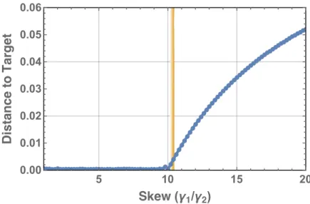
II.3 Strength of reachability conditions on a generalised amplitude damping Lindbladian . . . 55

II.4 Non-symmetric qutrit in a Λ configuration . . . 56

II.5 Reachability of non-symmetric Λ qutrit systems . . . 57

III.1 Method for constructing minimal dilations . . . 64

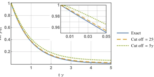
III.2 Effect of introducing a finite cut off to the dilation of the phase-flip channel 73 III.3 Dilation for an amplitude damping channel with resonant driving . . . 75

IV.1 Non-commutativity of tracing away the bath and adding controls . . . 78

IV.2 Truncating Taylor expansion for calculating modified Friedrichs-Lee model . 89 IV.3 Commutativity of modified Friedrichs-Lee model with qubit rotation . . . . 90

IV.4 Violation of the LCC conjecture in modified Friedrichs-Lee model . . . 91

V.1 Classical and quantum computer performing in situ control . . . 98

V.2 Steps in finding an optimal set of controls in situ . . . 102

V.3 Comparison of the gate fidelity with the local estimator of the fidelity . . . 107

V.4 Optimisation cost for different couplings and topologies . . . 111

V.5 Scaling of optimisation cost in an Ising chain . . . 112 V.6 Comparison of optimisation cost between neighbouring and distant qubits . 113

(8)

VI.1 Three-qubit Shor Code . . . 119

VI.2 Encoding step for the five-qubit code . . . 120

VI.3 Collective dephasing energy structure . . . 121

VI.4 Steps for in situ error correction. . . 122

VI.5 Recovering the three-qubit Shor code . . . 125

VI.6 Correcting unknown errors . . . 126

VI.7 Recovering the five-qubit stabiliser code . . . 127

VI.8 Obtaining a DFS from continuous collective dephasing noise . . . 128

(9)

GLOSSARY

The following notation is used through out the thesis, and is summarised here for conve-nience.

Symbol Name Description

H Hilbert Space

|ψi Pure State |ψi ∈H

d Dimension Dimension of the Hilbert space and states in it

ρ Quantum State ρ=P_p

i|ψii hψi|

T Time-ordering Operator _T[x(t1)x(t2)] =x(t2)x(t1) t1≤t2

+h.c. Hermitian Conjugate Shorthand to include the Hermitian conjugate

σi Pauli Matrices Canonical Pauli matrices,σ0=I

σ+(σ−) Raising (Lowering) Operator σ+|0i=|1i, σ+|1i= 0 (σ−|0i= 0, σ−|1i=|0i) I Identity Operator I|v_i=_|v_{i ∀ |}v_i I Identity Map _I(ρ) =ρ _∀ρ M(_·) Quantum Channel ρ(t) =M[ρ(0)] U(_·) Unitary Channel _U(ρ) =U ρ U† G(_·) Generator ρ˙=G(ρ) H(_·) Hamiltonian Generator _H(ρ) =₋i[H, ρ] L(·) Lindbladian Generator L(ρ) =−i[H, ρ] +P kγk h VkρVk†−12{V † kVk, ρ} i

G0, H0, L0 Drift Uncontrollable part of the generator

Kk Kraus Operator M(ρ) =PKkρKk†

P

Kk†Kk =I

|Ωi Bell Entangled State |Ωi=√1

d

Pd

i=1|ii ⊗ |ii

ρM Choi State ρM = (M ⊗ I)|Ωi hΩ|

S Vectorised Vectorised super-operator ˜

S Frame Change Operator/super-operator in a different frame

S Unital Unital block of super-operator

U(d) (SU(d)) (Special) Unitary Group U U†₌_I _|_det_U_|_{= 1 (det}_U _{= 1)} O(d) (SO(d)) (Special) Orthonormal Group OOT ₌

I |detO_|= 1 (detO= 1)

u(d) (su(d)) (Special) Unitary Algebra Lie algebra ofU(d) (SU(d))

o(d) (so(d)) (Special) Orthonormal Algebra Lie algebra ofO(d) (SO(d))

λ

λλ(_·) Eigenvalues Eigenvalues of an operator/super-operator

σ

σσ(·) Singular values Singular values of an operator/super-operator

≺ Majorization Partial order between sets (defined in Eq.(II.4))

F(M, U) Gate Fidelity F(M, U) = Tr[ρMρU] =hψ|ρM|ψi

(10)

(11)

CHAPTER I

INTRODUCTION

I.A

Overview

I.A.1 General Motivation

The laws of quantum mechanics are weird and wonderful. They predict things, that have been experimentally verified to astonishing precision, which cannot be explained by any physical model that obeys basic common sense principles [HBDRK15]. This is because such common sense about how the world ought to behave is based on experience of the macroscopic world of billiard balls, springs, and planets. Delving into the microscopic world of atoms, electrons, and photons requires a fundamentally new understanding of physics, and even logic.

Quantum mechanics has been around from the start of the previous century, but since Feynman’s landmark paper [Fey82] there has been a drive to understand it from a computational viewpoint and to harness it to do useful things. This new field is loosely called ‘Quantum Information’ or ‘Quantum Technology’ depending on whether the focus is on a better understanding of quantum behaviour or on its application. It has had a remarkable growth since the turn of the millennium and is still accelerating; new journals in this area are appearing almost every year [EPJ14, IOP15, NPJ15, Ope17] and it has attracted large amounts of funding from both the public and private sector [EPS14, Eur16, MRNBD17, IBM17, Mic17].

The potential uses of quantum technology fall into three broad categories: cryptogra-phy, sensing, and computation. Of these cryptography is the most advanced as it is already commercially available [SGGRZ02] and has even been used in satellites [LYLSL17]. The basic idea is to generate a shared random key between two parties (which can then be used to perfectly encrypt information sent between them) in such a way that any potential eavesdropper leaves a statistical trail that gives them away. Quantum sensing involves the construction of exotic quantum states that are highly sensitive to some external param-eter, such as gravity, allowing it to be measured far more accurately and efficiently than

(12)

CHAPTER I. INTRODUCTION

otherwise possible. It is less developed but has already been used in gravitational wave detectors [AAAAA13] and is seen as an achievable short-term goal for more prosaic tasks such as detecting pipes beneath the ground [BBCFH16]. Lastly is quantum computation, the holy grail of the field. Algorithms have been developed for a quantum computer that can solve certain problems vastly faster than even the most powerful conventional com-puter, doing in a fraction of a second what would otherwise take billions of years [DE98]. A universal quantum computer that could run any such algorithm reliably is probably not going to be available in the immediate future, but more specialised ones that can simulate other quantum systems would also be of use, and already exist on a small scale [BR12, LBRdLM16, SSBCM16, OBKRM16, MMHHL16]. Even this more limited goal is of revolutionary significance as it would allow molecular or solid-state systems to be simulated, understood, and even designed to have specific properties.

Making machines capable of achieving these tasks is of course difficult; there are nu-merous theoretical and experimental hurdles to overcome. Many of these centre around two questions, “How do imperfections affect the system?” and “How can the system be manipulated?” The first question brings in the notion of open systems. These take into account the imperfections of the real world: noise arising from vibrations in the experi-mental set up, stray electric or magnetic fields, and general thermal effects from the rest of the universe interacting with the system at hand. Such effects can never be eliminated completely so it is important to understand their impact and how to mitigate them or even use them beneficially. The second question is the topic of control theory which addresses both controllability (“what control knobs does a machine need to accomplish a task?”) and optimal control (“what is the best way of using these control knobs to do it?”). This thesis investigates the overlap of these two questions and asks what a quantum system can do in the presence of noise, and how it can be made to do it. Answering these questions not only paves the way to better quantum technology, but also sheds new light on natural quantum processes.

I.A.2 Context

As the research we did is on the overlap between open systems and control theory, it is worthwhile to first discuss what both terms mean in this context. Open quantum systems are those which are not isolated from the rest of the universe and so do not solely obey the Schr¨odinger equation. The system is governed by more than just a Hamiltonian and can undergo a broader range of evolutions which, crucially, can be used to take into account the myriad of ways that the environment affects it [BP02, RH11]. This normally acts to deteriorate and destroy the fragile quantum states that are useful for information processing and so is considered noise. The environment is everything that the system is in contact with but external to it. By its very nature it is something that cannot be controlled directly, if it could be then it would be considered part of the system itself rather than

(13)

I.A. OVERVIEW

an outside influence. For example, if an experimentalist could remove or set to a desired value all electromagnetic fields in the laboratory, then those fields would be taken as part of the system and not the environment. In this thesis, therefore, controlling open quantum systems means controlling systems in the presence of noise, rather than directly changing the noise in the system itself (as others have considered [SHMFKL12, BWSH16]).

There are nevertheless a lot of different ways of controlling a quantum system. A control is anything that can be tuned or applied to the system in order to modify its behaviour. The type of control most used in this thesis is Hamiltonian based: adding an extra (time-dependent) term to the Hamiltonian of the system in order to make it evolve in the desired way [D’A08]. This is usually done experimentally by creating an extra classical field, such as a laser pulse, that interacts with the system in a known and tunable way. The other type of control considered here is the use of ancillas; these are additional systems initialised in a certain state that interact with the system and are then discarded. For a set of allowed controls, whatever they may be, a natural aim is to find all possible tasks that can be accomplished: this is the topic of controllability or reachability [D’A08, Ell09]. As it is generally difficult to implement lots of different controls in an experiment, finding the minimal set which can do the required tasks is of practical use, as is showing that some systems are more flexible than others. The second aspect of control theory is optimal control, which finds a set of controls that reach a desired objective best in terms of fidelity or some other constraint. A common use for this is to find control pulses, such as the shape of a laser, used to drive a quantum system to do a particular logic gate [GBCKK15].

In this thesis, the control of open quantum systems is focussed on finite dimensional systems. That is, although the source of dissipation may be a bath in an infinite dimen-sional Hilbert space, the system being controlled itself resides in finite dimensions. This allows some of the results from the control of closed quantum systems to be applied, as well as the use of a matrix description of quantum mechanics. As most proposals for quantum technology make use of discrete degrees of freedom, this is also the most relevant for the field. The control tasks that are investigated are all on the level of operators (unitaries, quantum channels, or Lindbladians), rather than on creating a particular state. This is the most powerful for quantum information processing as it gives the ability to act on any input state in the desired way, allowing such operations to be chained together arbitrarily. It also reproduces the results of state control provided that the initial state is known.

The remainder of this chapter covers the general background necessary to follow the thesis. This includes how to describe open quantum systems mathematically, and some of their properties in§I.B; while major results and common methods in quantum control theory are introduced in_§I.C. More specialised discussion of existing state of the art results are left to the beginning of the relevant chapters where our original research is presented. In §II the question of controllability in the presence of fixed noise is investigated and

(14)

results in no-go theorems where the anisotropy of the dissipative dynamics is a resource which can be used to reach different target operations. This can be used as a method to simulate other open systems, a problem which is also tackled in§III. In that case there is no intrinsic noise in the system, but the use of time-dependent Hamiltonians and ancillas allows open dynamics to be replicated continuously in time. This is also an example of how unitary controls can modify the noise felt by a system. A conjecture about when this does not happen, which also investigates some of the earlier assumptions made, is proposed in §IV where our investigation of it is discussed. The last two chapters take these, and previous, ideas about what can be done with quantum control and finds a powerful way of calculating what the required values of the optimal controls are. The idea is to let quantum machines learn how to control themselves; in§V this is used to find logic gates for a quantum simulator, and in_§VI to implement tailor made error correcting codes.

I.B

Background on Open Quantum Systems

Open quantum systems are, as mentioned above, those whose evolutions are not sim-ply governed by unitary propagators and Hamiltonian generators due to their interaction with an external environment. This causes more general dynamics to take place than that described by the Sch¨odinger equation, including loss of coherence and dissipation of information. Such lossy behaviour is termed noise and is usually an unwanted affect in experiments investigating quantum behaviour or in attempts to build quantum tech-nologies. It is nevertheless present and hard to remove, making it important to take into account such effects explicitly when working with models of quantum systems. This allows protocols to be designed which either mitigate the effect of noise or use it as a resource, for example to cool the system or to simulate other open dynamics.

A review of the formalism used to describe open systems in terms of super-operators is given here in order to introduce to the reader the key physical and mathematical concepts that are used thereafter; this also serves to fix the notation that will be used. This introduction is based on a number of standard texts [BP02, BZ06, RH11]. It begins by discussing how to generalise the description of how closed quantum systems evolve in order to take into account external noise and loss of quantum information. An axiomatic definition of such quantum channels is given, which is then showed to be related to standard unitary evolution over a larger space. The question of whether such channels can be broken into small pieces such that a continuous evolution in time is well defined is addressed, which naturally gives rise to a definition of Markovianity for quantum systems. A derivation of how such dynamics can be calculated from an interaction between a system and its bath is then presented. Finally, some methods used to describe these linear operators as matrices, and their properties, are given. There exist other methods to describe open quantum systems that are not used in presenting our results later on, and so are not introduced,

(15)

I.B. BACKGROUND ON OPEN QUANTUM SYSTEMS

including: quantum stochastic equations [HP84a, Gre01] and the SLH formalism [CKS17], and hierarchical equations of motion [XCLMY05, XXCLY07].

I.B.1 Generalising Unitary Evolution

In closed quantum systems, the state at a given time|ψ(t)i is related to the initial state

|ψ(0)_i according to _|ψ(t)_i=U_|ψ(0)_i, whereU is a unitary propagator obeyingU U†₌_I_.

To generalise this to open systems, it is useful to first consider the same equation acting on a density operatorρ. These represent mixed states and are a convex mixture of pure states, ρ=X i pi|ψii hψi| where pi>0, X i pi = 1. (I.1)

They can be interpreted as being a probabilistic mixture: the system has probability pi

of being in state _|ψii, and the expectation value of some operator P over it is simply

given by Tr[P ρ]. From this definition, ρ has three important properties. It is Hermitian, positive semi-definite (all its eigenvalues are non-negative real numbers), and has trace one. Furthermore, all operators with these properties are valid states. Under this formalism, unitary evolution is expressed as

ρ(t) =U ρ(0)U†≡ U[ρ(0)], (I.2) where the last equality defines the super-operator_U, which is the Adjoint action ofU onρ. One of the most fundamental questions of open systems is to find what other propagators (also known as dynamical maps or quantum channels) are allowed that give physically sensible evolutions.

For a dynamical mapM to be physical, it needs to map any quantum state to another quantum state. In addition to it being linear that requires three properties, similar to those given for quantum states,

M(ρ) =M(ρ)† (I.3a)

Tr[M(ρ)] = 1 (I.3b)

M_{⊗ I}d(ρ⊗Id)≥0, (I.3c)

for allρ and where Iis the identity matrix,I is the identity map, and in the last line an additional ancillary system of dimensiondis added. The first condition simply states that

M maps Hermitian operators to Hermitian operators, this is clearly necessary in order forM(ρ) to be a valid state as defined above. Similarly for the second property of trace preservation.

The last condition is the most interesting one, in the case of d = 1 (such that the ancillary system is trivial) it defines a positive map: one that maps positive operators

(16)

to positive operators. The extension of it to an additional ancillary system of arbitrary dimension defines a completely positive map. The physical justification for it is that it is not enough to require thatM maps an isolated physical state to another physical state; it must also be the case that applying the map to one system while doing nothing to another system also results in a physical state. It is a surprising result of quantum mechanics that not all positive maps are completely positive. Fortunately, it is not necessary to check over all possible multipartite input states and over all possible extensions of the dynamical map to determine complete positivity, it is sufficient to consider the single case of the ancilla having the same dimension as the system, and for the larger map to act trivially (_I) on it. Dynamical maps that satisfy all these properties are called completely positive and trace preserving (CPT).

A property that some, but far from all, quantum channels have is unitality. This is the preservation of the maximally mixed state (ρ = _d1I): a quantum channel is unital if and only if

M(I) =I. (I.4)

As the maximally mixed state represents a system with maximum uncertainty, and is invariant under unitary transformations, this is a property which comes up regularly in quantum information.

One way of expressing a quantum channel is in terms of its Kraus representation. This states that a dynamical map can always be written in the form

M(ρ) = R X k=1 Kkρ Kk† where R X k=1 K_k†Kk=I, (I.5)

where theK are the Kraus operators and R is the Kraus rank of the map and is upper bounded by d2. This relation holds both ways; any set of Kraus operators for which

P

K_k†Kk = I gives rise a CPT map. From this it is easy to see that unitary evolution

also falls under this framework, it consists of CPT maps with a Kraus rank of one. If the quantum channel is unital, then the Kraus operators also obeyP

KkKk†=I.

An important relation between quantum channels and states is given by the Choi-Jamio lkowski isomorphism. This states that there is a one-to-one correspondence between the space of CPT maps and quantum states on the doubled space. The meaning of this is more readily apparent from the transformation that goes from a channel to an (unnormalised) state, which is

ρM = (M⊗ I)|Ωi hΩ| where |Ωi= d

X

i=1

|i_{i ⊗ |}i_i, (I.6) where_{|i_i}is a basis set for the system and ancilla. The Choi stateρM of a CPT mapMis

(17)

can be interpreted as linking correlations in time (the dynamical map) to correlations in space (the state). One practical benefit of this isomorphism is that it provides a simple way to determine whetherM is completely positive: M is completely positive if and only ifρM is positive semi-definite [BZ06].

I.B.2 Unitary Dilation

The previous section provided an axiomatic approach to determining which dynamical maps are physically sensible. Another approach is to follow the ‘Church of the Larger Hilbert Space’ as coined by John Smolin. This states that, ignoring measurements, the Schr¨odinger equation is all there is and that all evolutions are unitary. Things appear to be open because only a restricted subsystem is being observed, the underlying physics driving the system are unitary on a larger Hilbert space.

To formulate what this means for open systems it is necessary to first introduce the partial trace. This is defined over a bipartite system as the only linear operator for which

TrB[XA⊗YB] =XTr[Y] ∀ X∈HA, Y ∈HB, (I.7)

where HA,HB are the Hilbert spaces of the two parts of the system. That is, it ‘traces

out’ one subsystem while preserving the other. Applied to a product stateρ=ρA⊗ρB it

simply removes one of the subsystems while leaving the other unchanged. For more general states, such as entangled ones, it provides an average of the remaining state weighed by the one being traced out. Physically, it represents loss of information about the space being traced out and causes an entangled state to become a mixed one. It is a useful tool to focus the mathematical description of a quantum state to the part of the system that can be directly manipulated in the lab and remove the inaccessible environment. This also reduces the complexity of the description from one over potentially infinite degrees of freedom to the smaller system of interest.

With this, it is possible to formulate the open evolution of one system as a Stinespring dilation M(ρS) = TrA h U ρS⊗ρAU† i , (I.8)

where ρS is the system of interest, ρA is an ancillary system and U is a joint unitary

over both. This precisely formulates a quantum channel as unitary evolution on a large space followed by loss of information about part of the system. One restriction of this approach is that it requires the system and ancilla to start in a product state; this ensures that the resulting map is linear and well defined. There are attempts to go around these assumptions in [RRMAG10, Pec94], but this gives rise to new problems and remains controversial (as discussed in comments on the latter reference [Ali95, Pec95]).

(18)

maps given in Eq.(I.3) and Eq.(I.8) are equivalent. Every CPT map that obeys the conditions given in Eq.(I.3) has a Stinespring dilation which allows it to be expressed as Eq.(I.8), where the dimension of the ancillary space is at least the Kraus rank of the channel. Moreover, the two descriptions are truly interchangeable in that allM which are of the form Eq.(I.8) are CPT maps. This is a reassuring result: it confirms that complete positivity and trace preservation are indeed sensible properties to ask for open quantum systems, and that everything can be considered as unitary on a large enough space.

I.B.3 Generators of CPT Maps

The previous two sections extended the concept of a propagator from the unitaries of closed quantum dynamics to the dynamical maps of open quantum systems. It is natural to do the same thing for another class of important operators - Hamiltonians. In closed systems these describe the dynamics of the system, that is, not the evolution from one point in time to another single point in time, but the whole path it takes in the Hilbert space. They are related to the evolution of unitaries according to (~is set to 1 throughout the thesis)

d

dtU(t) =−iHU(t) or equivalently U(t) =e

−iHt_, _(I.9)

and give the evolution of states according to

d

dtρ(t) =−i[H, ρ(t)]≡ H[ρ(t)], (I.10)

where the last equality defines the super-operator _H, which is the adjoint action of H

on ρ. In this case the unitaries are a function of time, so a Hamiltonian generates a one parameter group of unitary matrices (that is any set{U(t)} which has the property

U(t2)U(t1) =U(t1+t2) for allt∈R). Due to the Lie group property of unitaries (discussed

in more detail in§I.C.1) the statement can also be reversed: any one parameter group of unitary matrices can be expressed as an exponential of a Hamiltonian. The situation is slightly more complex if the Hamiltonian is time-dependent

d dtU(t) =−iH(t)U(t) or equivalently U(t) =T exp −i Z τ 0 dτ H(τ) , (I.11)

whereT is the time-ordering operator, but the principle result is the same: all unitaries are exponentials of Hamiltonians.

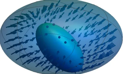
It is desirable to have an operator with similar properties in open systems, a generator which when exponentiated gives a CPT map, as shown in Fig.I.1. However this cannot always be done; the relation between propagator and generator is lost in the case of dynamical maps due to the requirement for complete positivity. In order to adapt the idea of generators to open systems it is necessary to see which quantum channels belong

(19)

Figure I.1|Illustration of the action of a CPT map and its generator on a high dimensional state space. The outer ellipsoid represents the state space att= 0, while the inner ellipsoid is the same state space at a later time, after it has been acted on by a CPT map. The space has undergone a linear transformation and has shrunk. The generator for that quantum channel is represented by the arrows, it shows how the state space evolves att = 0; integrating this flow leads to the recovery of the dynamical map.

to a one parameter semigroup

{Mt:Mt2Mt1 =Mt1+t2 ∀t1, t2≥0}, (I.12)

where Mt2Mt1 is a concatenation of maps. They will not form a group as non-unitary

quantum channels cannot be undone by another quantum channels because loss of in-formation is irreversible. This semigroup property is studied in [WC08] where different classes of CPT maps are introduced based on their divisibility. The maps that are most similar to unitaries are the infinitely divisible ones which have the property

M =M_nn _∀ n_∈N, (I.13)

stating that the mapM is identical to a different mapMn (itself CPT) actingntimes. It

might be expected that such a property would imply that the map is of the formMt=eLt.

This is indeed the case. Furthermore the generatorL has a specific structure,

L(ρ) =₋i[H, ρ] +X k γk VkρV_k†− 1 2{V † kVk, ρ} , (I.14)

where H is an ordinary Hamiltonian, γk > 0, the Vk are referred to as Lindblad or

jump operators, and L itself is the Lindbladian [Kos72, GKS76, Lin76]. The form of the dynamical map as the exponential of this gives rise to the celebrated

(20)

Gorini-Kossakowski-CHAPTER I. INTRODUCTION

Sudarshan-Lindblad equation on either the operator or state level

d

dtMt=LMt

d

dtρ(t) =L(ρ(t)). (I.15)

Such evolution is called Markovian, although different definitions of the word exist based on different concepts [BLP09, RHP14, BD16]. For the purpose of this thesis, open systems described by Eqs.(I.14-I.15) are called time-independent Markovian.

A slight generalisation of the infinitely divisible channels are the infinitesimally divisible ones. These can also be expressed as an infinite concatenation,

M =

n

Y

i=1

Mi ∀ n∈N, (I.16)

but the maps into which they are broken down are no longer required to be identical (but are still CPT). Such dynamical maps also belong to a semigroup and have a generator, but it is now time-dependent. In the same way as for time-dependent Hamiltonians, the evolution of the propagated can be described by

d dtMt=LtMt or equivalently M(t) =T exp −i Z t 0 dτ Lτ . (I.17)

The generator, L, has the same structure as in Eq.(I.14) except that the γ and Vk are

allowed to be dependent. Unsurprisingly, such systems are referred to as time-dependent Markovian.

Not every quantum channel, however, has these properties. Even for qubits (quan-tum bits with d = 2), the majority of maps are not Markovian [WECC08]. The most extreme are the non-divisible CPT maps, they are those which cannot be expressed as the concatenation of two CPT maps

M ₆=M2M1 (I.18)

where neitherM1 orM2 are purely unitary.

From the divisibility properties required of them, the Lindblad generators given here give rise to CPT maps between any two points in time, that is, the propagator that maps the system from timet1 tot2,

Mt2,t1 =T exp −i Z t2 t1 dτ Lτ , (I.19)

is CPT for allt2 > t1. It is possible to impose a weaker requirement, that only the CPT

map acting fromt= 0 to a later time is CPT and that the dynamics are time-local

Mt=T exp −i Z t 0 dτ Gτ , (I.20)

(21)

where G is a more general generator not necessarily of Lindblad form. The physical reasoning behind considering such dynamics is that it allows memory effects, where the evolution of the system attis influenced by its past evolution. Although a much broader ranged of CPT maps admit such a form (though still not all of them); adding a Hamiltonian

Hon the system on top ofGin Eq.(I.20) can result in loss of complete positivity for certain evolution times. It is therefore generally not clear what the physical meaning of G is in this case and, especially in a control scenario where Hamiltonians are commonly added, need to be treated with care. Nevertheless, they are a useful way of describing a wide-class of non-Markovian systems.

Unitality as defined in Eq.(I.4) was a useful property for quantum channels as it cate-gorised the maps that left the maximally mixed state invariant. It is similarly convenient to define it for generators. The desired behaviour is for unital generators to give rise to only unital CPT maps, which naturally leads to the definition

G(I) = 0, (I.21)

for unital generators, and the same for unital Lindbladians. Hamiltonian evolution is, of course, always unital.

I.B.4 Microscopic derivation of Lindbladians

The generators of Lindblad type, introduced in the previous section in Eq.(I.14), give rise to semigroups of CPT maps and therefore occupy a similar role in open quantum dynamics as Hamiltonians play for closed systems. The physical meaning of this generator, or how it arises from an interaction with another system in the same way as CPT maps arise from a unitary on a larger space, is not at all evident from the definition given previously. It is however possible, with certain assumptions, to start with a system interacting with a bath via a Hamiltonian and derive a Lindbladian on the system alone; one way of doing so is shown below following well known methods [BP02, RH11].

The starting point is to consider the system to be in contact with a bath. A bath in this context means an environment or an ancilla with a great number of degrees of freedom, such as a quantum field, with which the system is coupled. It is also typically in a thermal state. The system and the bath have the joint Hamiltonian

H=H0+HI =HS⊗I+I⊗HB+HI, (I.22)

where the first two terms act solely on the system and bath respectively while the latter is an interaction between them. This interaction term is treated separately because the isolated dynamics of the system and bath are assumed to be known and solved. As in the case of Eq.(I.8), the initial state is assumed to be in a product state,ρ(0) =ρS(0)⊗ρB(0).

(22)

Without loss of generality, it is also possible to assume that Tr[HIρ(0)] = 0 by shifting

terms between the Hamiltonians.

The first step to calculate an equation of motion for ρS(t) only is to move to the

interaction picture, denoted by a tilde,

˜

HI(t) =eiH0tHIe−iH0t, (I.23)

and ˜ρ(0) = ρ(0). The Schr¨odinger equation applied to density operators give rise to the Liouville-Von Neumann equation, Eq.(I.10); using this in the interaction picture and formally integrating it with respect to time gives

˜

ρ(t) =ρ(0)₋i Z t

0

[ ˜HI(τ),ρ˜(τ)]dτ. (I.24)

This can then be substituted back into the Liouville-Von Neumann equation, essentially doing a series expansion up to the second term

d dtρ˜(t) =−i[ ˜HI(t), ρ(0)]− Z t 0 [ ˜HI(t),[ ˜HI(τ),ρ˜(τ)]]dτ (I.25) d dtρ˜S(t) =−iTrB h [ ˜HI(t), ρ(0)] i − Z t 0 TrB h [ ˜HI(t),[ ˜HI(τ),ρ˜(τ)]] i dτ, (I.26)

where the bath was traced out to get to the last line.

To proceed further a number of different assumptions have to be made which together form the Born-Markov approximation. First, the bath is assumed to be in a fixed state for during the entire evolution: ρ(t) =ρS(t)⊗ρB. This cannot be exactly true if the two

systems are truly interacting and ρS is becoming less pure, but it is nevertheless a good

approximation in many cases. This is because the bath is considered to be large compared to the system, and so any back-action caused to it is small. Due to this, the system is memoryless as correlations built up between the system and the bath decay much faster that the dynamics of the system. This is similar to the discussion in the previous section where the evolution of the open system depended only on its current state and not on the past; this allowsρS(τ) inside the integral of Eq.(I.26) to be replaced byρS(t) and extends

the limit of the integral to +_∞. Finally, by noting that TrB[[ ˜HI(τ), ρ(0)]] = 0 due to the

definition ofHI, the dynamics ofρS(t) can be expressed as the Markovian master equation

d dtρ˜S(t) =− Z ∞ 0 TrB h [ ˜HI(t),[ ˜HI(t−τ),ρ˜S(t)⊗ρB]] i dτ. (I.27)

This is an equation of motion for ρS(t) (albeit in the interaction picture) which only

depends on its current state, the initial state of the bath, and the Hamiltonian coupling them together. This is not quite yet sufficient to show that this equation describes the generator of a CPT semigroup.

(23)

Some further manipulations, as well as a secular approximation, is required to obtain the Lindblad equation, which are sketched out here. The interaction Hamiltonian,HI can

always be decomposed as a sum of tensor products of Hermitian operators

HI =

X

α

Aα⊗Bα. (I.28)

This caries forward in the interaction picture

˜ HI(t) = X α eiHSt_A αe−iHSt⊗eiHBtBαe−iHBt= X α ˜ Aα(t)⊗B˜α(t). (I.29)

It is advantageous to transform the system operatorsAα(t) to be functions of frequency,

ω, such that

[HS, Aα(ω)] =−ωAα(ω) and [HS, A†α(ω)] =ωA†α(ω), (I.30)

which allows the interaction Hamiltonian to be recast as

˜ HI(t) = X α,ω ˜ Aα(ω)⊗B˜α(t), (I.31) where hBα(t)i= Tr[Bα(t)ρB] = 0, (I.32)

from the original constraint that Tr[HIρ(0)] = 0. Substituting this into Eq.(I.27) gives,

after some algebraic manipulation,

d dtρ˜S(t) =− X ω,ω0 X α,β e−i(ω0−ω)tΓα,β(t, ω) Aβ(ω)˜ρS(t)A†α(ω0)−A†α(ω0)Aβ(ω)˜ρS(t) +h.c., (I.33)

where h.c. is the Hermitian conjugate and the Γ are the one sided Fourier transform of the bath correlation functions

Γα,β(t, ω) =

Z ∞

0

dτ eiωτTr[B†_α(t)Bβ(t−τ)ρB]. (I.34)

From the Born-Markov approximation, the state of the bath is fixed, therefore the corre-lation function are unchanged by a shift in time and so the previous expression simplifies to

Γα,β(ω) =

Z ∞

0

dτ eiωτTr[B_α†(τ)Bβ(0)ρB]. (I.35)

The final approximation to make is to only consider the terms in Eq.(I.33) whereω =ω0_.

This is a rotating-wave (also called secular) approximation similar to Born-Markov made earlier: terms oscillating rapidly compared to the evolution of the system are averaged out

(24)

and ignored. Put together this yields

d dtρ˜S(t) =− X ω X α,β Γα,β(ω) Aβ(ω)˜ρS(t)A†α(ω0)−A†α(ω0)Aβ(ω)˜ρS(t) +h.c. (I.36)

The last step is to transform out of the interaction picture and split the Γ into Hermitian and anti-Hermitian parts

Γα,β(ω) =

1

2(γα,β+iSα,β(ω)). (I.37) Finally, this gives

d dtρS(t) =−i[HLS+HS, ρS(t)] +D(ρS(t)] (I.38) where HLS = X ω X α,β Sα,β(ω)A†α(ω)Aβ(ω) D(ρS) = X ω X α,β γα,β(ω) Aβ(ω)ρSA†α(ω)− 1 2{A † α(ωAβ(ω), ρS} .

HLS is the Lamb shift, which is the extra energy the system has due to its interaction

with the environment. The dissipative part of the generator can be diagonalised and brought into the standard form of Eq.(I.14). It can be shown from properties of the Fourier transform and bath correlation functions that γα,β(ω) is positive semi-definite,

and therefore the decay rates are all positive. The result of Eq.(I.38) is therefore an evolution in time of the reduced system governed by a generator of Lindblad type, which was precisely the class of generators that gave rise to CPT semigroups.

This derivation shows that there is a clear link between the mathematical properties required by the generators of CPT semigroups, and the evolution of open systems interact-ing with a large bath that satisfies certain approximations. In the same way as Stinesprinteract-ing dilations provide a link between CPT maps and unitaries on a larger space, this is a reas-suring result that shows mathematical and physical approaches converge. It also highlights the assumptions that go into such a model and the regimes where open systems are not Markovian. Indeed, it should be noted that the Born-Markov approximations as described above are not fully satisfactory. One problem is that they are an approximation and not an expansion, it is therefore not clear how higher order terms could be calculated in or-der to check that they are sufficiently small. This can be circumvented by more detailed calculations in some models [DL05]. A different problem is that the approximation made leads to exponential decay, which is approximately linear for short times. Yet any unitary dynamics can only lead to quadratic decay of population, as diagonal terms in the density matrix vary only in second order. This shows that the Born-Markov approximation result in some coarse-graining of the dynamics and should not be expected to resolve details happening on time scales shorter than the bath correlation time.

(25)

I.B.5 Vectorisation

The formalism used for finite dimensional closed quantum systems is usually linear algebra, specifically: states are column vectors and operators are matrices. This is a very convenient formulation both for algebraic manipulations and for numerical simulations. The way to do this for open quantum systems is to transform density matrices into vectors, and the super-operators that act on them (quantum channels and generators) into matrices. This can be done with a technique called vectorisation [BZ06], which has close links with tensor network representations [CD11, WBC15].

The starting point is to work in the generalised Bloch representation, where a quantum stateρ is represented as the real vector

|ρ_i= (x1, x2, x3, ..., xd2)T where x_i= Tr[σ_iρ], (I.39)

are the expectation values over an orthonormal set {σi} which forms a basis over all

operators. The inverse map is simply given by

ρ=X

i

xiσi. (I.40)

The same thing can be done for a super-operatorS, where its vectorised form is denoted byS, according to S=Sij|ii hj| (I.41a) Sij = Tr[σ†_iS(σj)] (I.41b) S(ρ) =X i,j σiSijρj (I.41c) |S(ρ)_i=S_|ρ_i. (I.41d) This is a useful representation as the vectorised formShas the same linear algebra proper-ties as the parent super-operatorS. The spectral properties (eigenvalues, singular values, trace and determinant) ofS and S are the same, the dual of a super-operatorS†_{, defined}

according to Tr[µS(ρ)] = Tr[S†(µ)ρ], has as its matrix representation the Hermitian con-jugate of the matrix representation of the original super-operator, such that (S†) = (S)†, and the concatenation of two super-operators is given by the matrix product of their vectorised form.

One simple choice of basis for the {σi} is row-vectorisation. All the elements ofσi are

0 except for a single one, which has value 1; the basis is enumerated by the location of that element, going along each row and then downwards. Using such a basis, a general

(26)

CHAPTER I. INTRODUCTION qubit state is ρ= ρ00 ρ01 ρ10 ρ11 ! −→ |ρi= (ρ00, ρ01, ρ10, ρ11)T, (I.42)

such that the rows of the matrix are simply listed one after the other. A nice property of this basis, known as Roth’s Lemma, is

ABC _−→A_⊗CT _|B_i, (I.43)

which is particularly powerful to vectorise entire equations. The Choi-Jamio lkowski iso-morphism of Eq.(I.6) is also very straightforward in this representation and can be done by ‘reshuffling’ elements,ρM =MR, where reshuffling is defined as

S_mµ,nνR =Smn,µν, (I.44)

where the first two indices label the row element over the bipartite system, and the last two the column element. This is eminently more clear with an example for a qubit channel and a two-qubit Choi state:

ρM =MR=       M00 M01 M10 M11 M02 M03 M12 M13 M20 M21 M30 M31 M22 M23 M32 M33       . (I.45)

Another particularly useful choice of for the{σi}are traceless Hermitian matrices for

i= 2, ..., d2_{, and}_σ

1 = √1_dI. The Pauli matrices and the identity are the natural choice for

such a basis, which highlights that vectorisation is just a Bloch representation for higher dimensions. A consequence of this is that Hermitian operators and super-operators are real when vectorised this way. As they are particularly important, the form that the super-operators of closed dynamics take in this representation are described here, which touches on elements of Lie groups discussed below in§I.C.1. Unitary propagators, U(·) =U ·U†, become matrices in the defining representation of the rotation group I1 ⊕SO(d2 −1).

Hamiltonian generators,_H(_·) =₋i[H,_·], are in the corresponding Lie algebra, 01⊕so(d2−

1), which consist of real antisymmetric (and therefore traceless) matrices. In the case of

d= 2, unitary propagators form all such matrices (and like-wise for Hamiltonians), but in higher dimension they only form a subgroup. This means that ind= 2 only, the set of every unitary on the system corresponds to all possible rotations of the state vector|ρi. In higher dimensions however, there exist rotations of this vector which cannot be induced by any Hamiltonian controls on the system; this is analoguous to saying that not every vector in the generalised Bloch space is a valid quantum state.

(27)

(a) Dephasing (b)Amplitude Damping

Figure I.2|Illustration of the Bloch sphere under two common types of qubit noise. The first is a unital dephasing channel, which preserves mixtures of the _|0_i and

|1_i states but destroys superpositions. The second is an amplitude damping channel where all states decay to the ground state_|0_i.

I.B.6 Common types of qubit noise

There are two different types of common qubit noise that are typical of dissipative pro-cesses: dephasing and amplitude damping. These, or variants of these, will be used throughout this thesis as examples and it is useful to have a visualisation of what they do. A convenient way of picturing their effect is to plot how they transform the Bloch sphere, as is done in Fig.I.2.

Possibly the simplest type of qubit noise is dephasing, where the probability of being in two states (usually picked as|0i and |1i) is conserved, but phase information between them is lost. This type of noise is also sometimes called pure decoherence as it does not degrade classical information, as such it is unital, and in many cases is the dominant type of noise. One physical way it can occur is when the energy splitting in a qubit fluctuates in some unknown way, and it corresponds to theT2 decoherence time commonly quoted

in NMR. The Lindbladian for it is

L(ρ) =₋γ[σz,[σz, ρ]], (I.46)

and a state_|ψ_i=α_|0_i+β_|1_i evolving under it will tend to

ρ=|α|2|0i h0|+|β|2|1i h1|, (I.47) with the off-diagonal terms decaying exponentially, as is sketched in Fig.I.2a. In a micro-scopic derivation of the type done in§I.B.4, such noise typically arises from the interaction between the system and the low frequency part of the bath.

Another common type of noise is amplitude damping, where all points in the Bloch sphere decay to the ground state. Unlike dephasing, such noise has a single fixed point and

(28)

destroys classical, as well as quantum, information. It is the typical example of non-unital qubit noise and in many ways is as different to dephasing as possible; phase information is lost by the system at the minimum rate, constrained by the decay to the ground state and complete positivity. In can be interpreted as a qubit cooling down to absolute zero, or as an atom undergoing spontaneous emission. The Lindbladian for it is

L(ρ) =₋γ(_{σ+σ−, ρ} −2σ−ρσ−), (I.48)

and a state evolves, as shown in Fig.I.2b, according to

|α|2 _αβ∗ α∗β |β|2 ! −→ |α| 2₊_|_β_|2₍₁₋_e−2γt₎ _αβ∗_e−γt α∗βe−γt |β|2_e−2γt ! . (I.49)

While theT2noise described above comes from the low frequency part of the bath, energy

conservation constraints show that the T1 type of noise described by amplitude damping

arises from the modes of the bath which are close to resonance with the qubit internal energy splitting.

I.C

Background on Quantum Control

Control theory, in the context of quantum mechanics, is about how the ability to vary certain parameters in a system allows different operations to be reached. There are two main types of controls considered throughout this thesis: Hamiltonians that can be varied in time, and the ability to add and discard ancillary systems. The latter is completely binary and is used exclusively at the start or end of the dynamics; it is therefore considered separately from the ability to vary Hamiltonians during the evolution of the system.

In this formulation, a control system consists of a Hamiltonian

H(t) =H0+

X

k

fk(t)Hk, (I.50)

whereH0 is the drift Hamiltonian, theHk are the control Hamiltonians, and thefk(t) are

called the control parameters or pulse interchangeably. Control theory investigates how the choice of the controls affect the unitary that can be reached

U(t) =_T exp −i Z t 0 H(τ)dτ . (I.51)

In the common case of constant controls, the Hamiltonian itself is also piecewise-constant and so the above expression simplifies to

U(t) = N Y n=0 exp −iH nt N t N , (I.52)

(29)

I.C. BACKGROUND ON QUANTUM CONTROL

whereN is picked such that the Hamiltonian is constant over the intervalT /N and the n

are sorted with the lowest value to the right in the product.

Control theory can also be used in the context of state control, where the objective is to map a stateρ1toρ2. The work in this thesis focusses entirely on operator control so this

branch of control theory is not presented here, the methods used in any case are very similar and the result is that operator controllability implies state controllability (but not the reverse). It also possible to do feedback control, where the system is continuously measured as it is evolves and the controls are adjusted based on the results [DJ99, DHJMT00, WD05]. This is not a method considered in this thesis, although the in situ method proposed in

§V and_§VI does involve measuring the system after it has finished evolving.

The principle results of controllability of closed quantum systems, preceded by a brief introduction of the key requisite notions of Lie groups and algebras, are presented below following the lines of [D’A08, Ell09, Nak03] and the author’s MRes thesis on the same project [Div14]. A short discussion of why this approach does not work in the case of either open or infinite dimensional systems is also included. This is followed by a way of finding what values the control parameters need to take to achieve a given goal, the topic of optimal control, focussing on a particular algorithm GRAPE [KRKSHG05] implemented in Python on QuTiP [JNN13, JNPGG16] that we used repeatedly in our research.

I.C.1 Some properties of Lie groups and algebras

The dynamics of closed quantum systems are, as has already been touched on in _§I.B, highly dependent on Lie properties linking Hermitian operators (the Hamiltonians) to unitary operators (the propagators). The fundamental representation of the unitary group U(d) consists of ddimensional complex matrices U, with the property thatU U†₌_I _and

|detU_|= 1. Hermitian matrices, H, are trivially those for whichH=H†. An important concept for control theory is thatUis a Lie group, rather than just a group, and therefore the corresponding Hamiltonians form a Lie algebra.

A Lie group is a group where every element is also a point on a smooth manifold, such that the group operation and the inverse are smooth maps on the manifold. The matrix groups, such asU(d), have this property. To define a lie algebra it is necessary to consider a curveX(t) on a Lie group Gsuch that X(t) _∈G_∀t_∈R and X(0) =I. The direction explored by the curve att= 0 is defined by

x= d

dtX(t)|t=0. (I.53)

Taking all possible curvesX(t) on G leads to many different x which together form the Lie algebra g, also known as the tangent space of G. This Lie algebra is a vector space

(30)

overRwhich has an additional map

[·,·] :g_×g_→g, (I.54) called the Lie bracket. This obeys a series of properties

[αx+y, z] =α[x, z] + [y, z] (I.55a) [x, y] =₋[y, x] (I.55b) [x,[y, z]] + [y,[z, x]] + [z,[x, y]] = 0, (I.55c)

which are all satisfied by the usual matrix commutator [A, B] = AB−BA. It is worth pointing out that the dimension ofGas group and as a manifold is equal to that of g.

In the same way that Eq.(I.53) provides a map from a curve on the Lie group to an element of the associated algebra, the reverse can be done by defining the exponential map as

exp (xt) =X(t), (I.56)

whereX(t) is a one parameter subgroup ofG. The usual matrix exponential satisfies this property. Just as all curves on G give all elements of g, the Lie group can be generated by the Lie algebra according to

G=eg ={ex1_ex2_...exm _|_x

1, x2, ..., xm∈g}. (I.57)

A visualisation of this is given by a heuristic geometrical picture. Each element of the Lie group G corresponds to a point on a smooth differentiable manifold. The Lie algebra g corresponds to the set of tangent vectors at the identity element of G: the different directions that can be explored from the identity. As such, an element ofg leads to a vector flow in G; by starting at the identity and moving along it a one parameter subgroup ofGis generated. The commutator [x1, x2] is the vector displacement of moving

an infinitesimal amount along x1 followed by x2, compared to moving along x2 followed

byx1; this itself is a direction inGand therefore an element ofg.

The link between this and quantum mechanics comes by identifyingGwithU(d), the trajectory X(t) with the propagator U(t), and elements of g with Hamiltonians −iH. The presence of the ₋i is one that depends on convention, mathematicians often prefer to work directly with elements of the Lie algebra and so define Hamiltonians to be anti-Hermitian; this will not be done here in order to maintain the usual physical significance of Hamiltonians as energy operators. The result is that, to apply Lie theory to quantum mechanics,−ineeds to be inserted in front of xin Eq.(I.53) and Eq.(I.56). Indeed, doing this shows how similar those equations are to the operator version of the Schr¨odinger equation.

(31)

Adopting this convention, the Lie algebra associated with the unitary group U(d) is

u(d) which is composed of allddimensional Hermitian matrices. As global phases are of no physical importance in quantum mechanics, it is often useful to work with slightly different groups. These are the special unitariesSU(d) which have the stronger requirement that detU = 1. The associated algebra is su(d) and is formed of all traceless Hermitian matrices. The equivalent groups also exist in the case of real matrices (as encountered in

§I.B.5): the special orthogonal groupSO(d) consists of real rotation matrices O such that

OOT =I and detO = 1, and its algebraso(d) made up of antisymmetric real matrices.

I.C.2 Reachability of Closed and Finite Quantum Systems

The definitions above, and especially Eq.(I.57) state that, if all Hamiltonians can be implemented with controls, then every propagator can be reached. This is an enormously strong requirement that is very rarely realised in any physical situation. In practice, a much smaller set of control Hamiltonians can be used to reach the space of all unitaries. A physically motivated illustration of what this set is, although not a formal proof, is outlined below.

It is instructive to begin by formally writing down the reachable set

R= ( Te−iRH(t)dt|H(t) =H0+ X k fk(t)Hk ∀fk(t) andt≥0 ) , (I.58)

which is all the unitaries at any (positive) time that can can be generated by the Hamil-tonian. A trivial observation is that the exponential of any Hamiltonian with constant controls fk(t) = fk is in the reachable set. By increasing the evolution time, positive

multiples of the Hamiltonian can be created. While the controls may allow for thefk(t)

to be negative, it is not immediately obvious that the sign of H0 can be reversed. This

can in fact also be done by using the quantum recurrence theorem [BL57] which states that, becauseU(d) is a compact group,

∀H, _∃tr > T : ||e−iHtr −I||< , (I.59)

where _||._|| is any matrix norm. This states that there always exists a time (above any minimum time) such that the system has evolved arbitrarily close to the identity. This permits the system to effectively evolve backwards in time by evolving for long enough forward in time

e−iH(−t) 'e−iH(tr−t) _where _t

r> t, (I.60)

up to some small error. Thus, if e−iH is in the reachable set, then so ise−iHt for all t. Another observation can be made by invoking the Trotter formula (a lemma of the

(32)

CHAPTER I. INTRODUCTION Baker-Campbell-Hausdorff formula) e−i(A+B)t= lim n→∞ e−nitAe −it n B n , (I.61)

stating that the sum of two Hamiltonians can be exponentiated by alternating between the exponential of the two individual Hamiltonians. Combining this with the previous result, the exponential of any Hamiltonian which is in the linear space spanned byH(t) is in the closure of the reachable set, where the closure is used to include elements that are

close to being reachable. This space can be further expanded by using another lemma of the BCH formula, the commutator relation

e−[A,B]t2 = lim n→∞ e−nitAe −it n Be it nAe it nB n2 , (I.62)

which states that the exponential of the commutator of A and B can be reached by alter-nating between exponentiating those two directions forward and backwards in time. As it has already been shown that this can be done, the reachable set includes the exponential of the commutator ofH(t).

By combining the ability to scale Hamiltonians, take linear combinations, and com-mutators iteratively the whole Lie algebra

L= * H(fk) =H0+ X k fkHk + Lie , (I.63)

(rather than just the vector space) spanned by the control Hamiltonians is in the closure of the reachable set. Furthermore, this is exactly the reachable set [D’A08, Ell09], such that

R=eL, (I.64)

is the set of all unitary matrices that can be reached arbitrarily well by the control system of Eq.(I.50). In order to determine whether U(d) is reachable it is therefore sufficient to calculate the dimension of the Lie algebra L; if this is d2 or d2 −1 (the dimension of U(d) and SU(d) respectively) then the system is fully controllable. In the case that the dimension is lower only a subgroup ofU(d) can be reached, as these are limited in number, the dimension of the Lie algebra is a good indicator of what the reachable set is. This dimension is easy to compute as it is composed of nothing but linear combinations and commutators.

The Lie algebra criterion is not, however, a practical constructive method for how thefk(t) need to be chosen in order to reach a desired unitary. The use of the quantum

recurrence theorem implies waiting a significant amount of time to reach negative times, and both Eq.(I.61) and Eq.(I.62) require an unbounded number of repetitions. This would therefore require huge evolution time before getting close to a desired unitary and for the

(33)

controls to be very high frequency, neither of which are desirable. Different methods, typ-ically numerical, have to be used to find the required pulse. Before giving an introduction to such a method, a brief explanation of why this criteria fails for open or infinite systems is presented.

The approach taken here fails for open systems at the first hurdle. The space of CPT maps, even when limited to just the Markovian ones which admit a generator, form a semigroup but not a group. The physical reason for this is that CPT maps represent a loss of coherence, there is information flowing out of the system. Any concatenation of CPT maps cannot only lead to information being recovered. Without this group structure, the whole construction presented here falls apart. It can be partially recovered by defining Lie semigroups and related objects, this gives rise to a limited set of results for open systems [DHKSH09, ODSH12]; these are discussed in the context of a different method to determine controllability introduced in_§II.

One way around such difficulties would be to treat the open system as a larger unitary one. The environments which are of physical interest are almost always infinitely dimen-sional, thus the problem of open control can be mapped to infinite dimensional control, although the question of which dilation should be used is subtle. The key step in the construction of the reachable set presented above that fails for such systems is in evolving for negative time using the recurrence theorem of Eq.(I.59). In mathematical terms, this is because unitary groups in infinite dimensions are not compact. Geometrically this can be seen as the Lie group in finite dimensions being curved (like the Bloch sphere ind= 2) such that evolution in any direction eventually leads back to the identity, while in infinite dimension the evolution goes on forever without curving back. A simple physical explana-tion of this is to consider a particle in one dimension evolving according to the momentum operator, U(t) =e−ipt_{, there is no value of} _{t >} _{0 for which this approaches the identity.}

Nevertheless, in the case of quadratic Hamiltonians, the rank criteria described here can be used with only small modifications [GSKB12].

I.C.3 Methods in Optimal Control

As discussed above, the Lie algebraic condition is an efficient way of determining which unitaries can be reached by a quantum control system. It is, however, not constructive and provides little insight as to what fk(t) in Eq.(I.50) needs to be in order to reach a

target unitaryUT. This problem is the topic of optimal control, where iterative numerical

methods are used to find a control pulse that achieves the desired goal, and the description here is based around well established methods [MSGdFG11, GBCKK15]. As this approach does not use the analytic properties of Lie groups, it can also be used for open or infinite dimensional systems, and with minimal modifications also applies to state control (where many of the algorithms were actually first developed).

(34)

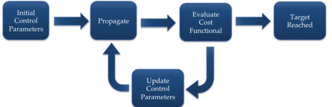
The steps for finding the controls for a unitary are outlined in Fig.I.3. The starting point is an initial set of values for control parameters, including the total evolution time and value offk(t). In order to have a finite number of control parameters, those are usually

taken as piecewise-constant [KRKSHG05], or are expressed in a Fourier basis with a finite number of components [DCM11, CCM11, MTWA15] . If there is no a priori knowledge as to what the control pulse ought to be, the values of the parameters are chosen randomly. The evolution of the system with these parameters is then calculated in order to obtain

Ufk(t), the unitary that is generated by the controls. This requires obtaining an accurate

model for the system (the values ofH0 andHk, as well as the generator of the noise if the

system is open) and then solving the time-dependent Schr¨odinger equation numerically for a model of the system. If the system is fully controllable, such a simulation will be exponentially difficult as it scales with the dimension of the entire Hilbert space. In small systems, this can however be done without undue difficulty. The algorithm then needs a cost functional

F[fk(t), UT], (I.65)

which determines how far the current controls are from realising the desired operation. The simplest choice for this is the gate fidelity

FU = Tr[Ufk(t)U

†

T] or FSU =|Tr[Ufk(t)U

†

T]|, (I.66)

depending on whether the global phase of the evolution matters or not respectively; this common choice is why the cost functional is often called the fidelity. Additional terms to the cost functional can be added in order to encourage the pulse to have certain properties, for example adding a cost proportional to theL1 norm results in sparser control pulses or a

maximum value can be imposed; this is used to include physical constraints on the desired pulses. If the value ofF[fk(t), UT] is above a certain threshold, the target fidelity, then the

scheme terminates and the values of the control parameters which achieved the desired operation are recorded. If this is not the case, the value of the control pulses (either all of them simultaneously or a subset at a time) are updated, and the process loops around. If a random initial pulse was taken, the whole process would generally be repeated with different initial pulses, as the final fidelity reached (and the number of iterations required to find it) depends strongly on the initial values.

How to update the control pulse is a completely classical problem and countless tech-niques that have been developed in computer science and statistics can be used here. One class of methods are called simplex, such as Nelder-Mead [NM65], which starts by eval-uating the functional at n points in the parameter space that form a simplex and picks the next point to evaluate as a linear combination of the previous ones, weighed by their fidelity. The protocol then repeats itself, taking the bestn points in each iteration when guessing the next one. A different approach is to use a genetic algorithm, where differ-ent values of the control parameters are randomly mutated and the most successful are