17
Workload-Aware Anonymization Techniques
for Large-Scale Datasets
KRISTEN LeFEVRE University of Michigan DAVID J. DeWITT Microsoft and RAGHU RAMAKRISHNAN Yahoo! Research
Protecting individual privacy is an important problem in microdata distribution and publishing. Anonymization algorithms typically aim to satisfy certain privacy definitions with minimal impact on the quality of the resulting data. While much of the previous literature has measured quality through simple one-size-fits-all measures, we argue that quality is best judged with respect to the workload for which the data will ultimately be used.
This article provides a suite of anonymization algorithms that incorporate a target class of workloads, consisting of one or more data mining tasks as well as selection predicates. An extensive empirical evaluation indicates that this approach is often more effective than previous techniques. In addition, we consider the problem of scalability. The article describes two extensions that allow us to scale the anonymization algorithms to datasets much larger than main memory. The first extension is based on ideas from scalable decision trees, and the second is based on sampling. A thorough performance evaluation indicates that these techniques are viable in practice.
Categories and Subject Descriptors: H.2.8 [Database Management]: Database Applications General Terms: Algorithms, Performance, Security
Additional Key Words and Phrases: Databases, privacy, anonymity, data mining, performance, scalability
ACM Reference Format:
LeFevre, K., DeWitt, D. J., and Ramakrishnan, R. 2008. Workload-aware anonymization techniques for large-scale datasets. ACM Trans. Datab. Syst. 33, 3, Article 17 (August 2008), 47 pages. DOI= 10.1145/1386118.1386123 http://doi.acm.org/10.1145/1386118.1386123
This research was conducted while the authors were at the University of Wisconsin – Madison. The work was partially supported by a grant from NSF CyberTrust and an IBM Ph.D. Fellowship. Author’s address: K. LeFevre (corresponding author), University of Michigan; email: klefevre@ eecs.umich.edu.
Permission to make digital or hard copies of part or all of this work for personal or classroom use is granted without fee provided that copies are not made or distributed for profit or direct commercial advantage and that copies show this notice on the first page or initial screen of a display along with the full citation. Copyrights for components of this work owned by others than ACM must be honored. Abstracting with credit is permitted. To copy otherwise, to republish, to post on servers, to redistribute to lists, or to use any component of this work in other works requires prior specific permission and/or a fee. Permissions may be requested from Publications Dept., ACM, Inc., 2 Penn Plaza, Suite 701, New York, NY 10121-0701 USA, fax+1 (212) 869-0481, or [email protected].
C
2008 ACM 0362-5915/2008/08-ART17 $5.00 DOI 10.1145/1386118.1386123 http://doi.acm.org/ 10.1145/1386118.1386123
1. INTRODUCTION
Numerous organizations collect, distribute, and publish microdata (personal data in its nonaggregate form) for purposes that include demographic and public health research. Typically, attributes that are known to uniquely identify indi-viduals (e.g., name or social security number) are removed from these datasets. However, data distributors are often concerned with the possibility of using external data to uniquely identify individuals. For example, according to one study, 87% of the population of the Unites States can be uniquely identified on the basis of their 5-digit zip code, sex, and date of birth [Sweeney 2002b]. Thus, even if a person’s name is removed from a published record, it may be possible to learn the identity of the person by linking the values of these attributes to an external source of information (e.g., a voter registration database [Sweeney 2002b]).
Conventional wisdom indicates that we can limit the risk of this kind of rei-dentification by removing certain attributes and coarsening the values of other attributes (e.g., time and geography). For example, the U.S. Health Insurance Portability and Accountability Act (HIPAA) Privacy Rule [HIP 2002] lays out specific attributes that must be removed from medical records when distribut-ing data under a limited use agreement, or more strictly when constructdistribut-ing a deidentified dataset for broader distribution. While they do not satisfy the letter of the HIPAA regulation,k-Anonymity [Samarati 2001; Sweeney 2002b],
-diversity [Machanavajjhala et al. 2006], and extensions [Xiao and Tao 2006; Martin et al. 2007; Chen et al. 2007] represent formalizations of the same in-tuition.
Subject to the given anonymity constraints, it is of course important that the data remain as useful as possible. It is our position that the best way of measuring quality is based on the task(s) for which the data will ultimately be used. This article proposes using a workload (including data mining tasks and queries) as an evaluation tool. We then develop a suite of techniques for incorpo-rating a target family of workloads into the anonymization process. In addition, we substantially extend our previous work [LeFevre et al. 2006a; LeFevre et al. 2006b] by providing a unified framework that allows these algorithms to scale to datasets significantly larger than main memory.
1.1 Problem Setting
Our proposal is best illustrated through a series of examples. Consider an or-ganization that compiles a database of disease information which could prove useful to external researchers. At the same time, it is important for the agency to take precautions protecting the privacy of patients, for example, hiding the identities of individuals and protecting other sensitive information such as HIV status.
The data distribution procedure can take on a variety of forms, and the amount of trust placed in the data recipient(s) can vary significantly. At one extreme, the data recipient could be a researcher whose work is subject to ap-proval by an Institutional Review Board (IRB) and who has signed a limited use agreement. While it is prudent to apply some anonymization to this data (e.g.,
as indicated informally by the HIPAA rule) to prevent passive reidentification by a rogue user, the risk is fairly low. At the other extreme, the agency might wish to post its data on a public website, in which case the eventual recipient(s) are unknown and comparatively less trustworthy.
Now consider Alice, a researcher who is directing two separate studies. As part of the first study, Alice wants to build a classification model that uses age, smoking history, and HIV status to predict life expectancy. In the second study, she would like to find combinations of variables that are useful for predicting elevated cholesterol and obesity in males over age 40. We consider the problem of producing a single sanitized snapshot that satisfies a given set of privacy requirements but that is useful for the set of tasks in the specified workload.
One might envision a simpler protocol in which Alice requests specific models constructed entirely by the agency. However, in many exploratory data mining tasks (e.g., Chen et al. [2005]), the tasks are not fully specified ahead of time. Perhaps more importantly, the inference implications of releasing multiple pre-dictive models (e.g., decision trees, Bayesian networks, etc.) are not well under-stood. It is well known that answering multiple aggregate queries may reveal more precise information about the underlying database [Adam and Wortmann 1989; Kenthapadi et al. 2005]. Similarly, each predictive model reveals some-thing about the agency’s data. On the other hand, it is appealing to release a single snapshot because there are well-developed notions of anonymity, and the best Alice can do is approximate the distribution in the data she is given.
Finally, it is important to consider the potential risk and implications of collusion. For example, suppose that Bob is the director of another laboratory carrying out a different set of studies and that he requests a separate dataset tailored towards his work. If Alice and Bob were to combine their datasets, they would likely be able to infer more precise information than was intended by the agency. In certain cases (e.g., in the presence of limited use agreements), the risk of collusion by two or more malicious recipients may be sufficiently low to be considered acceptable. In other cases (e.g., publication of data on the web), this is unrealistic. Nevertheless, it is often still useful to tailor a single snapshot to an anticipated class of researchers who are expected to use the data for similar purposes (e.g., AIDS or obesity research). In other words, in this case, we can produce a sanitized snapshot based on the anticipated workloads of all expected recipients with the expectation that this is the only snapshot to be released.
1.2 Article Overview and Contributions
This article is organized as follows. Section 2 reviews some common defini-tions of anonymity with respect to linking attacks and gives a brief overview of generalization and recoding techniques.
Our first main technical contribution, described in Section 3, is a simple lan-guage for describing a family of target workloads and a suite of algorithms for incorporating these workloads into the anonymization process when generat-ing a sgenerat-ingle anonymized snapshot. It is important to note that, unless special care is taken, publishing multiple sanitized versions of a dataset may be dis-closive [Kifer and Gehrke 2006; Wang and Fung 2006; Yao et al. 2005; Xiao
and Tao 2007]. In this article, we do not address the complementary problem of reasoning about disclosure across multiple releases.
We provide an extensive experimental evaluation of data quality in Section 4. The results are promising, indicating that often we do not need to compromise too much utility in order to achieve reasonable levels of privacy.
In Section 5, we turn our attention to performance and scalability, and we describe two techniques for scaling our proposed algorithms to datasets much larger than main memory. An experimental performance evaluation in Section 6 indicates the practicality of these techniques.
The article concludes with discussions of related and future work in Sec-tions 7 and 8.
2. PRELIMINARIES
Consider a single input relation R, containing nonaggregate personal data. As in the majority of previous work, we assume that each attribute in R can be uniquely characterized by at most one of the following types based on knowledge of the application domain.
—Identifier.Unique identifiers (denotedID), such as name and social security number are removed entirely from the published data.
—Quasi-Identifier.The quasi-identifier is a set of attributes available to the data recipient through other means. Examples include the combination of birth date, sex, and zip code.
—Sensitive Attribute.An attributeSis considered sensitive if an adversary is not permitted to uniquely associate its value with an identifier. An example is a patient’s disease attribute.
Throughout this article, we consider the problem of producing a sanitized snapshot R∗ of R. It is convenient to think of R∗ as dividing R into a set of nonoverlapping equivalence classes, each with identical quasi-identifier val-ues. Throughout this article, we will assume multiset (bag) semantics unless otherwise noted.
2.1 Anonymity Requirements
Thek-anonymity requirement is quite simple [Samarati 2001; Sweeney 2002b]. Intuitively, it stipulates that no individual in the published data should be identifiable from a group of size smaller thankon the basis of its quasi-identifier values.
Definition2.1 (k-Anonymity). Sanitized viewR∗is said to bek-anonymous if each unique tuple in the projection ofR∗onQ1,. . .,Qdoccurs at leastktimes. Althoughk-anonymity is effective in protecting individual identities, it does not take into account protection of one or more sensitive attributes [Machanava-jjhala et al. 2006]. -Diversity provides a natural extension, incorporating a nominal (unordered categorical) sensitive attributeS. The-diversity principle requires that each equivalence class in R∗ contain at leastwell-represented values of sensitive attribute S and can be implemented in several ways
[Machanavajjhala et al. 2006]. Let DS denote the (finite or infinite) domain of attribute S. The first proposal requires that the entropy of S within each equivalence class be sufficiently large. (We adopt the convention 0 log 0=0.)
Definition 2.2. Entropy -Diversity [Machanavajjhala et al. 2006] R∗ is entropy -diverse with respect to S if, for every equivalence class Ri in R∗,
s∈DS−p(s|Ri) logp(s|Ri)≥log(), where p(s|Ri) is the fraction of tuples inRi withS=s.
Entropy-diversity is often quite restrictive. Because the entropy function is concave, in order to satisfy-diversity, the entropy ofSwithin the entire dataset must be at least log(). For this reason, they provide an alternate definition motivated by an elimination attack model. The intuition informing the following definition is as follows: the adversary must eliminate at least−1 sensitive values in order to conclusively determine the sensitive value for a particular individual.
Definition 2.3. Recursive (c,)-Diversity [Machanavajjhala et al. 2006]. Within an equivalence classRi, letxi denote the number of times theith most frequent sensitive value appears. Given a constantc,Risatisfies recursive (c, )-diversity with respect toSifx1<c(x+x+1+ · · · +x|DS|).R∗satisfies recursive (c,)-diversity if every equivalence class inR∗satisfies recursive (c,)-diversity. (We say (c, 1)-diversity is always satisfied.)
When S is numerically-valued, the definitions provided by Machanava-jjhala et al. [2006] do not fully capture the intended intuition. For exam-ple, suppose S = Salary, and that some equivalence class contains salaries
{100K, 101K, 102K}. Technically, this is considered 3-diverse; however, intu-itively, it does not protect privacy as well as an equivalence class containing salaries{1K, 50K, 500K}.
For this reason, we proposed an additional requirement, which is intended to guarantee a certain level of dispersion ofSwithin each equivalence class.1Let
Var(Ri,S)=|R1 i|
t∈Ri(t.S−S(Ri))
2denote the variance of values for sensitive attributeSamong tuples in equivalence classRi. (LetS(Ri) denote the mean value ofSinRi.)
Definition 2.4. Variance Diversity [LeFevre et al. 2006b] An equivalence classRiis variance diverse with respect to sensitive attributeSifVar(Ri,S)≥
v, wherevis the diversity parameter.R∗is variance diverse if each equivalence class inR∗is variance diverse.
2.2 Recoding Framework and Greedy Partitioning
In previous work, we proposed implementing these requirements using a multi-dimensional partitioning approach [LeFevre et al. 2006a]. The idea is to divide 1Variance diversity also satisfies the monotonicity property described in Machanavajjhala et al.
[2006]. See the appendix for a short proof. In concurrent work, Li et al. [2007] also considered a numeric sensitive attribute and proposed a related privacy requirement calledt-closeness.
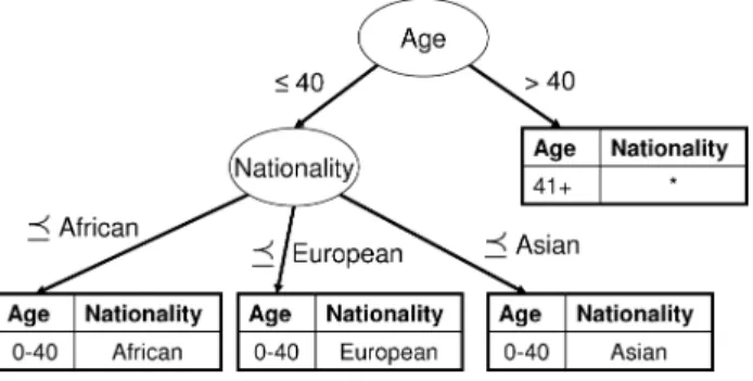
Fig. 1. Generalization hierarchy for nationality attribute.
Fig. 2. Example partition tree.
thed-dimensional quasi-identifier domain space into nonoverlapping rectangu-lar regions. This partitioning is then used to define aglobal recoding function
(φ:DQ1×· · ·×DQd →D
d) that maps each domain tuple to the region in which
it is contained.2φis then applied to the input relationRto produce R∗.
A partitioning is said to be allowable with respect to a particular in-put relation R if the recoded relation R∗, resulting from applying φ to the quasi-identifier attributes of R, satisfies all given anonymity requirements. The proposed algorithm (Mondrian) is based on greedy recursive partition-ing [LeFevre et al. 2006a]. Briefly, the recursive procedure takes as input a (potentially infinite) d-dimensional rectangular domain and a set of tu-ples, R. The algorithm chooses a quasi-identifier split attribute (dimension of the domain space). When the split attribute is numeric, the algorithm also chooses a binary split threshold (e.g., Age ≤ 40; Age > 40). For categorical attributes, the split is defined by specializing a user-defined generalization hi-erarchy (e.g., Figure 1) as originally proposed by Samarati [2001] and Sweeney [2002a]. We use the notation to indicate a generalization relationship. See Figure 2.
The split attribute (and threshold) define a division of the input domain into m nonoverlapping regions that cover the input domain. The split also defines a corresponding partitioning of the input data (R) into disjoint sub-sets, R1,. . .,Rm. The split is said to be allowable if eachRi satisfies the given anonymity requirement(s). For example, under k-anonymity, a split is allow-able if eachRicontains at leastktuples. The procedure is executed recursively on each resulting partition (Ri) until there no longer exists an allowable split. 2This is in contrast to other single-dimensional global recoding techniques which are defined by a
set of functionsφ1,. . .,φd such that eachφi: DQi →DQi.R
∗is obtained by applying eachφito
Informally, a partitioning is said to beminimalif it satisfies the given anonymity requirement(s), and there exist no further allowable splits.
When there is no known target workload, LeFevre et al. [2006a] proposed choosing the allowable split attribute with the widest (normalized) range of values and (for numeric attributes) used the median value as the threshold. We will refer to this simple algorithm as Median Mondrian. It is appealing because, underk-anonymity, if there exists an allowable split perpendicular to a particular axis, the split at the median is necessarily allowable and can be found in linear time. However, as we will show throughout this article, when there is a known workload, we can often achieve better data quality by replacing this split heuristic.
3. WORKLOAD-AWARE ANONYMIZATION
Our goal is to allow the data recipient to specify afamilyof target workloads, and we introduce a simple language for this purpose. In particular, a workload family is specified by one or more of the following tasks.
—Classification Tasks.A (set of) classification task(s) is characterized by a set of predictor attributes{F1,. . .,Fn}(also commonly calledfeatures), and one or more nominal class labelsC.
—Regression Tasks. A (set of) regression task(s) is characterized by a set of features{F1,. . .,Fn}and one or more numeric target attributesT.
—Selection Tasks.A set of selection tasks is defined by a set of selection predi-cates{P1,. . .,Pn}, each of which is a boolean function of the quasi-identifier attributes.
—Aggregation Tasks.Each aggregation task is defined by an aggregate function (e.g., SUM, MIN, AVG, etc.).
In the remainder of this section, we describe techniques for incorporating each of these components into the anonymization process.
3.1 Classification and Regression
We begin by considering workloads consisting of one or more classification or re-gression tasks. To lend intuition to the problem, consider a single classification or regression task and an anonymity requirement. Notice that each attribute has two characterizations: one for anonymity (QID, sensitive, or other), and one for the task (feature, target, or other).
For simplicity, suppose {Q1,. . .Qd} = {F1,. . .,Fn} (features and quasi-identifiers are the same), and consider a discrete class labelC. Intuitively, our goal in this case is to produce a multidimensional partitioning of the quasi-identifier domain space (also the feature space in this case) into regions con-taining disjoint tuple multisets R1,. . .,Rm. Each of these partitions should satisfy the given anonymity requirements. At the same time, because of the classification task, we would like these partitions to be homogeneous with re-spect toC. One way to implement this intuition is to minimize the conditional
entropy ofCgiven membership in a particular partition: H(C|R∗)= m i=1 |Ri| |R| c∈DC −p(c|Ri) logp(c|Ri). (1) This intuition is easily extended to a regression task with numeric target
T. In this case, we seek to minimize the weighted mean squared error which measures the impurity ofT within each partition (weighted by partition size). In the following,T(Ri) denotes the mean value ofT in data partition Ri.
WMSE(T,R∗)= 1 |R| m i=1 t∈Ri (t.T −T(Ri))2. (2)
The simple case, where the features and quasi-identifiers are the same, arises in two scenarios: It is likely to occur when the anonymity requirement is k -anonymity (i.e., no sensitive attribute), and it may also occur when the tar-get attribute (C or T) and sensitive attribute (S) are the same.3 Intuitively, the latter case appears problematic. Indeed, entropy -diversity requires that
H(C|R∗)≥log(), and variance diversity requires thatWMSE(T,R∗)≥v. That is, the anonymity requirement places a bound on quality.
In the remainder of this section, we first describe algorithms for incorporat-ing a sincorporat-ingle classification/regression model under the assumptions described (Section 3.1.1), and we extend the algorithm to incorporate multiple models (Section 3.1.2). Finally, in Section 3.1.3, we relax the initial assumption and describe a case where we can achieve high privacy and utility even when the sensitive attribute and target attribute are the same.
3.1.1 Single Target Model. Consider the case where {F1,. . .,Fn} =
{Q1,. . .,Qd}, and consider a single target classifier with class labelC. In order
to obtain heterogenous class label partitions, we propose a greedy splitting al-gorithm based on entropy minimization, which is reminiscent of alal-gorithms for decision tree construction [Breiman et al. 1984; Quinlan 1993]. At each recur-sive step, we choose the candidate split that minimizes the following function without violating the anonymity requirement(s). LetV denote the current (re-cursive) tuple set, and letV1,. . .,Vmdenote the set of data partitions resulting from the candidate split. p(c|Vi) is the fraction of tuples in Vi with class label
C=c. We refer to this algorithm as InfoGain Mondrian.
Entropy(V,C)= m i=1 |Vi| |V| c∈DC
−p(c|Vi) logp(c|Vi). (3) When we have a continuous target attributeT, the recursive split criterion is similar to the CART algorithm for regression trees [Breiman et al. 1984], choosing the split that minimizes the following expression (without violating 3Our approach is to release all attributes that are not part of the quasi-identifier (that are involved
in one of the tasks) without modification. In some cases, this includes the sensitive attribute. Thus, we must apply generalization to an attribute only if it is part of the quasi-identifier and either a feature or the target.
the anonymity requirement). We call this Regression Mondrian. Error2(V,T)= m i=1 t∈Vi (t.T−T(Vi))2. (4)
Each of the two algorithms handles continuous quasi-identifier values by partitioning around thethresholdvalue that minimizes the given expression without violating the anonymity requirement. In order to select this thresh-old, we must first sort the data with respect to the split attribute. Thus, the complexity of both algorithms isO(|R|log2|R|).
3.1.2 Multiple Target Models. In certain cases, we would like to allow the data recipient to build several models to accurately predict the marginal distributions of several class labels (C1,. . .,Cn) or numeric target attributes (T1,. . .,Tn). The heuristics described in the previous section can be extended to these cases. (For simplicity, assume{F1,. . .,Fn} = {Q1,. . .,Qd}.)
For classification, there are two ways to make this extension. In the first approach, the data recipient would build a single model to predict the vector of class labels,C1,. . .,Cn, which has domain DC1× · · · × DCn. A greedy split criterion would minimize entropy with respect to this single variable.
However, in this simple approach, the size of the domain grows exponentially with the number of target attributes. To avoid potential sparsity problems, we instead assume independence among target attributes. This is reasonable because we are ultimately only concerned about the marginal distribution of each target attribute. Under the independence assumption, the greedy criterion chooses the split that minimizes the following without violating the anonymity requirement(s):
n
i=1
Entropy(V,Ci). (5) In regression (the squared error split criterion in particular), there is no analogous distinction between treating the set of target attributes as a single variable and assuming independence. For example, if we have two target at-tributes,T1and T2, the joint error is the distance between an observed point (t1,t2) and the centroid (T1(V),T2(V)) in 2-dimensional space. The squared joint error is the sum of individual squared errors, (t1−T1(V))2+(t2−T2(V))2. For this reason, we choose the split that minimizes the following without violating the anonymity requirement(s):
n
i=1
Error2(V,Ti). (6)
3.1.3 Relaxing the Assumptions. Until now, we have assumed that
{F1,. . .,Fn} = {Q1,. . .,Qd}. In this case, if we have a sensitive attribute S
such thatS =C or S = T, then the anonymity requirement may be at odds with our notion of data quality.
However, consider the case where{Q1,. . .,Qd} ⊂ {F1,. . .,Fn}. In this case, we can draw a distinction between partitioning the quasi-identifier space
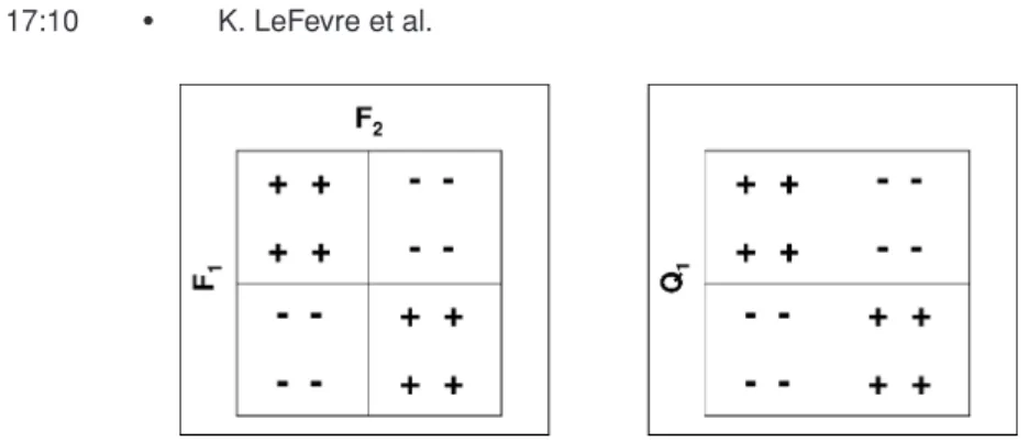
Fig. 3. Features vs. quasi-identifiers in classification-oriented anonymization.
and partitioning the feature space. For example, consider the partitioning in Figure 3 (with features F1,F2, and class labels/sensitive values+and−). The feature space partitions are homogeneous with respect to the class label. How-ever, suppose there is just one quasi-identifier attribute Q1=F1. Clearly, the partitioning is 2-diverse with respect toQ1.
This observation leads to an interesting extension of the greedy split heuris-tics. Informally, at each recursive step the extended algorithm chooses the (quasi-identifier) split that minimizes the entropy of C (or squared error of
T) across the resulting feature space partitions without violating the given anonymity requirement(s) across the quasi-identifier partitions.
3.2 Selection
Sometimes one or more of the tasks in the target workload will use only a subset of the released data, and it is important that this data can be selected precisely, despite recoding. For example, in Section 1.1, we described a study that involved building a model for only males over age 40, but this is difficult if the ages of some men are generalized to the range 30–50.
Consider a set of selection predicates {P1,. . .,Pn} defined by a boolean function of the quasi-identifier attributes{Q1,. . .,Qd}. Conceptually, each Pi
defines a query region Xi in the domain space such that Xi = {x : x ∈
DQ1× · · · ×DQd,Pi(x)=true}. For the purposes of this work, we only consider
selections for which the query region can be expressed as ad-dimensional rect-angle. (Of course, some additional selections can be decomposed into two or more hyper-rectangles and incorporated as separate queries.)
A multidimensional partitioning (and recoding function φ) divides the do-main space into nonoverlapping rectangular regionsY1,. . .,Ym. The recoding regionYi = {y : y ∈ DQ1× · · · ×DQd,φ(y)= yi∗}, where yi∗ is a unique
gener-alization of the quasi-identifier vector. When evaluating Pi over the sanitized viewR∗, it may be that no set of recoding regions can be combined to precisely equal query region Xi. Instead, we need to define the semantics of selection
queries on this type of imprecise data. Clearly, there are many possible seman-tics but, in the rest of this chapter, we settle on one. Under this semanseman-tics, a selection with predicatePireturns all tuples fromR∗that are contained in any
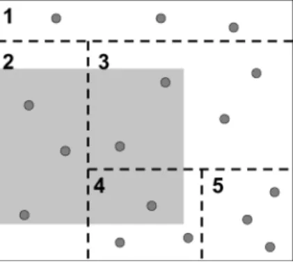
Fig. 4. Evaluating a selection over generalized data.
recoding region overlapping the corresponding query regionXi. More formally,
Overlap(Xi,{Y1,. . .,Ym}) = ∪{Yj :Yj ∈ {Y1,. . .,Ym},Yj ∩Xi = ∅}
Pi(R∗) = {φ(t) :φ(t)∈R∗∧t∈Overlap(Xi,{Y1,. . .,Ym})}. Notice that this will often produce a larger result set than evaluating Pi
over the original tableR. We define theimprecisionto be the difference in size between these two result sets.
Pi(R) = {t :t∈ R,Pi(t)=true}
imprecision(Pi,R∗,R) = |Pi(R∗)| − |Pi(R)|.
For example, Figure 4 shows a 2-dimensional domain space. The shaded area represents a query region, and the tuples ofR are represented by points. The recoding regions are bounded by dotted lines and numbered. Recoding regions 2, 3, and 4 overlap the query region. If we evaluated this query using the original data, the result set would include 6 tuples. However, evaluating the query using the recoded data (under the given semantics) yields 10 tuples, an imprecision of 4.
Ideally, the goal of selection-oriented anonymization is to find the safe (k-anonymous,-diverse, variance-diverse, etc.) multidimensional partitioning that minimizes the (weighted) sum of imprecision for the set of target predi-cates. (We assign each predicate Pi a positive weightwi.)
We incorporate this goal through another greedy splitting heuristic. LetV
denote the current (recursive) tuple set, and letV1,. . .,Vm denote the set of partitions resulting from the candidate split. Our heuristic minimizes the sum of weighted imprecisions:
n
i=1
wi∗imprecision(Pi,V∗,V). (7) The algorithm proceeds until there is no allowable split that reduces the imprecision of the recursive partition. We will call this algorithm Selection Mondrian. In practice, we expect this technique to be used most often for sim-ple selections, such as breaking down health data by state. Following this,
we continue to divide each resulting partition using the appropriate splitting heuristic (i.e., InfoGain Mondrian, etc.).
3.3 Aggregation and Summary Statistics
In multidimensional global recoding, individual data points are mapped to one multidimensional region in the set of disjoint rectangular regions covering the domain space. To this point, we have primarily considered representing each such region as a relational tuple based on its conceptual bounding box (e.g., see Figure 2).
However, when we consider the task of answering a set of aggregate queries, it is also beneficial to consider alternate ways of representing these regions using various summary statistics, which is reminiscent of ideas used in mi-croaggregation [Domingo-Ferrer and Mateo-Sanz 2002].4In particular, we con-sider two types of summary statistics which are computed based on the data contained within each region (partition). For each attribute Ain partitionRi, consider the following.
—Range Statistic (R).Including a summary statistic defined by the minimum and maximum value of Aappearing in Ri allows for easy computation of MIN and MAX aggregates.
—Mean Statistic (M). We also consider a summary statistic defined by the mean value of Aappearing in Ri, which allows for the computation of AVG and SUM.
When choosing summary statistics, it is important to consider potential av-enues for inference. Notice that releasing minimum and maximum statistics allows for some inference about the distribution of values within a partition. For example, consider an integer-valued attribute A, and letk = 2. Suppose that an equivalence class contains two tuples with minimum=0 and maximum=1. It is easy to infer that one of the original tuples has A=0 and, in the other, has
A=1. However, this type of inference is not problematic in preventing joining attacks because it is still impossible for an adversary to distinguish the tuples within a partition from one another.
4. EXPERIMENTAL EVALUATION OF DATA QUALITY
In this section, we describe an experimental evaluation of data quality; evalu-ation of runtime performance is postponed until Section 6.
Our experimental quality evaluation had two main goals. The first goal was to provide insight into experimental quality evaluation methodology. We out-line an experimental protocol for evaluating an anonymization algorithm with respect to a workload of classification and regression tasks. A comparison with the results of simpler general-purpose quality measures indicates the impor-tance of evaluating data quality with respect to the target workload when it is known.
4Certain types of aggregate functions (e.g., MEDIAN) are ill-suited to these types of computations.
The second goal is to evaluate the extensions to Mondrian for incorporating workload. We pay particular attention to the impact of incorporating one or more target classification/regression models and the effects of multidimensional recoding. We also evaluate the effectiveness of our algorithms with respect to selections and projections.
4.1 Methodology
Given a target classification or regression task, the most direct way of evalu-ating the quality of an anonymization is by training each target model using the anonymized data and evaluating the resulting models usingpredictive ac-curacy(classification), mean absolute error(regression), or similar measures. We will call this methodologymodel evaluation. All of our model evaluation experiments follow a common protocol. In particular, we consider it important to hold out the test set during both anonymization and training.
(1) The data is first divided into training and testing sets (or 10-fold cross-validation sets), Rtrainand Rtest.
(2) The anonymization algorithm determines recoding functionφ using only the training set Rtrain. Anonymous viewR∗trainis obtained by applyingφto
Rtrain.
(3) The same recoding functionφis then applied to the testing set (Rtest), yield-ingR∗test.
(4) The classification or regression model is trained using Rtrain∗ and tested usingRtest∗ .
Unless otherwise noted, we used k-anonymity as the anonymity require-ment. We fixed the set of quasi-identifier attributes and features to be the same, and we used the implementations of the following learning algorithms provided by the Weka software package [Witten and Frank 2005]:
—Decision Tree(J48). Default settings were used.
—Naive Bayes.Supervised discretization was used for continuous attributes; otherwise all default settings were used.
—Random Forests.Each classifier was comprised of 40 random trees, and all other default settings were used.
—Support Vector Machine(SMO). Default settings, including a linear kernel function.
—Linear Regression.Default settings were used. —Regression Tree(M5). Default settings were used.
In addition to model evaluation, we also measured certain characteristics of the anonymized training data to see if there was any correlation between these simpler measures and the results of the model evaluation. Specifically, we measured the average equivalence class size [LeFevre et al. 2006a], and for classification tasks, we measured the conditional entropy of the class label C, given the partitioning of the full input dataRintoR1,. . .,Rm(see Equation (1)).
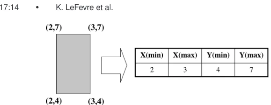
Fig. 5. Mapping ad-dimensional rectangular region to 2∗dattributes. 4.2 Learning from Regions
When single-dimensional recoding is used, standard learning algorithms can be applied directly to the resulting point data, notwithstanding the coarseness of some points [Fung et al. 2005]. Although multidimensional recoding techniques are more flexible, using the resulting hyper-rectangular data to train standard data mining models poses an additional challenge.
To address this problem, we make a simple observation. Because we restrict the recoding regions to include onlyd-dimensional hyper-rectangles, each re-gion can be uniquely represented as a point in (2∗d)-dimensional space. For example, Figure 5 shows a 2-dimensional rectangle, and its unique represen-tation as a 4-tuple. This assumes a total order on the values of each attribute similar to the assumption made by support vector machines.
Following this observation, we adopt a simple preprocessing technique for learning from regions. Specifically, we extend the recoding functionφ to map data points tod-dimensional regions, and, in turn, to map these regions to their unique representations as points in (2∗d)-dimensional space.
Our primary goal in developing this technique is to establish the utility of our anonymization algorithms. There are many possible approaches to the general problem of learning from regions. For example, Zhang and Honavar [2003] pro-posed an algorithm for learning decision trees from attribute values at various levels of a taxonomy tree. Alternatively, we could consider assigning a density to each multidimensional region, and then sampling point data according to this distribution. However, a full comparison is beyond the scope of this work.
4.3 Experimental Data
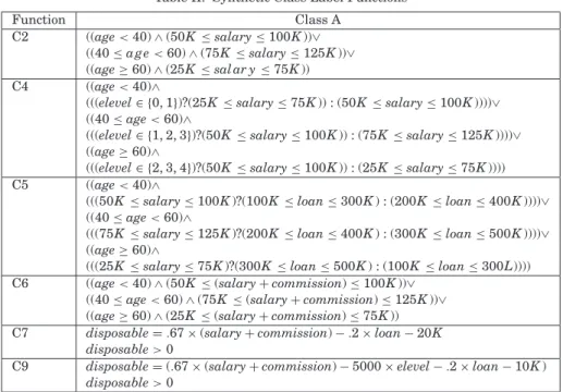
Our experiments used both synthetic and real-world data. The synthetic data was produced using an implementation of the generator described by Agrawal et al. [1993] for testing classification algorithms. This generator is based on a set of predictor attributes, and class labels are generated as functions of the predictor attributes (see Tables I and II).
In addition to the synthetic data, we also used two real-world datasets. The first (Table III) was derived from a sample of the 2003 Public Use Microdata, distributed by the United States Census American Community Survey5with target attribute Salary. This data was used for both classification and regression 5http://www.census.gov/acs/www/index.html.
Table I. Synthetic Features/Quasi-Identifier Attributes
Attribute Distribution
salary Uniform in [20,000, 150,000]
commission If salary≥75,000, then 0 Else Uniform in [10,000, 75,000]
age Uniform integer in [20,80]
elevel Uniform integer in [0, 4]
car Uniform integer in [1, 20]
zipcode Uniform integer in [0, 9]
hvalue zipcode *h* 100,000 wherehuniform in [0.5, 1.5]
hyears Uniform integer in [1, 30]
loan Uniform in [0, 500,000]
Table II. Synthetic Class Label Functions
Function Class A
C2 ((age<40)∧(50K≤salary≤100K))∨
((40≤a g e<60)∧(75K≤salary≤125K))∨ ((age≥60)∧(25K≤sal ar y≤75K)) C4 ((age<40)∧
(((elevel∈ {0, 1})?(25K≤salary≤75K)) : (50K ≤salary≤100K))))∨ ((40≤age<60)∧
(((elevel∈ {1, 2, 3})?(50K≤salary≤100K)) : (75K≤salary≤125K))))∨ ((age≥60)∧
(((elevel∈ {2, 3, 4})?(50K≤salary≤100K)) : (25K≤salary≤75K)))) C5 ((age<40)∧
(((50K≤salary≤100K)?(100K≤loan≤300K) : (200K≤loan≤400K))))∨ ((40≤age<60)∧
(((75K≤salary≤125K)?(200K≤loan≤400K) : (300K≤loan≤500K))))∨ ((age≥60)∧
(((25K≤salary≤75K)?(300K≤loan≤500K) : (100K≤loan≤300L)))) C6 ((age<40)∧(50K≤(salary+commission)≤100K))∨
((40≤age<60)∧(75K≤(salary+commission)≤125K))∨ ((age≥60)∧(25K≤(salary+commission)≤75K))
C7 disposable=.67×(salary+commission)−.2×loan−20K
disposable>0
C9 disposable=(.67×(salary+commission)−5000×elevel−.2×loan−10K)
disposable>0
and contained 49,657 records. For classification, we replaced the numeric Salary with a Salary class (<30K or≥30K); approximately 56% of the data records had Salary<30K. For classification, this is similar to the Adult database [Blake and Merz 1998]. However, we chose to compile this new dataset that can be used for both classification and regression.
The second real dataset is the smaller Contraceptives database from the UCI Repository (Table IV), which contained 1,473 records after removing those with missing values. This data includes nine socio-economic indicators, which are used to predict the choice of contraceptive method (long-term, short-term, or none) among sampled Indonesian women.
Table III. Census Data Description Attribute Distinct Vals Generalization
Region 57 hierarchy
Age 77 continuous
Citizenship 5 hierarchy
Marital Status 5 hierarchy
Education (years) 17 continuous
Sex 2 hierarchy
Hours per week 93 continuous
Disability 2 hierarchy
Race 9 hierarchy
Salary 2/continuous target
Table IV. Contraceptives Data Description Attribute Distinct Vals Generalization
Wife’s age 34 continuous
Wife’s education 4 hierarchy
Husband’s education 4 hierarchy
Children 15 continuous
Wife’s religion 2 hierarchy
Wife working 2 hierarchy
Husband’s Occupation 4 hierarchy
Std. of Living 4 continuous
Media Exposure 2 hierarchy
Contraceptive 3 target
4.4 Comparison with Previous Algorithms
InfoGain Mondrian and Regression Mondrian use both multidimensional re-coding and classification- and regression-oriented splitting heuristics. In this section, we evaluate the effects of these two components through a comparison with two previous anonymization algorithms. All of the experiments in this section consider a single target model constructed over the entire anonymized training set.
Several previous algorithms have incorporated a single-target classification model while choosing a single-dimensional recoding [Fung et al. 2005; Iyengar 2002; Wang et al. 2004]. To understand the impact of multidimensional recod-ing, we compared InfoGain Mondrian and the greedy Top-Down Specialization (TDS) algorithm [Fung et al. 2005]. Also, we compare InfoGain and Regres-sion Mondrian to Median Mondrian to measure the effects of incorporating a single-target model.
The first set of experiments used the synthetic classification data. Notice that the basic labeling functions in Table II include a number of constants (e.g., 75K). In order to get a more robust understanding of the behavior of the vari-ous anonymization algorithms, for functions 2, 4, and 6, we instead generated many independent datasets, varying the function constants independently at random over the range of the attribute. Additionally, we imposed hierarchical generalization constraints on attributes elevel and car.
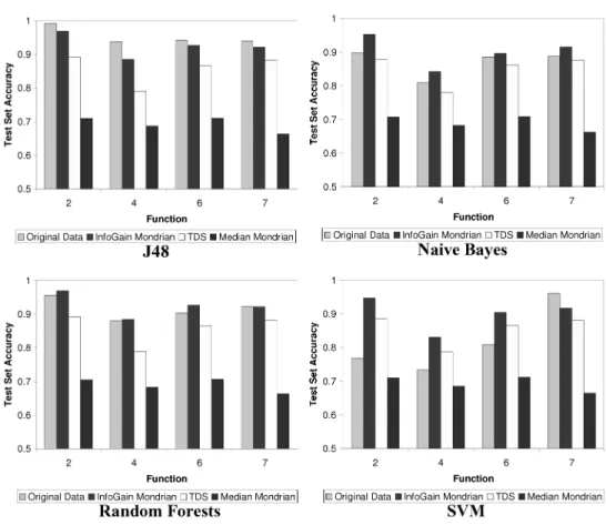
Figure 6 compares the predictive accuracy of classifiers trained on data pro-duced by the different anonymization algorithms. In these experiments, we
Fig. 6. Classification-based model evaluation using synthetic data (k=25).
generated 100 independent training and testing sets, each containing 1,000 records, and we fixedk=25. The results are averaged across these 100 trials. For comparison, we also include the accuracies of classifiers trained on the (not anonymized) original data.
InfoGain Mondrian consistently outperforms both TDS and Median Mon-drian, a result that is overwhelmingly significant based on a series of paired t-tests.6It is important to note that the preprocessing step used to convert re-gions to points (Section 4.2) is only used for the multidimensional recodings; the classification algorithms run unmodified on the single-dimensional recodings produced by TDS [Fung et al. 2005]. Thus, should a better technique be de-veloped for learning from regions, this would improve the results for InfoGain Mondrian, but it would not affect TDS.7
We performed a similar set of experiments using the real-world data. Figure 7 shows results for the Census classification data for increasingk. The graphs 6For example, when comparing InfoGain Mondrian and TDS on the J48 classifier, the one-tailed
p-value is< .001 for each synthetic function.
7Note that by mapping to 2∗ddimensions, we effectively expand the hypothesis space considered
by the linear SVM. Thus, it is not surprising that this improves accuracy for the nonlinear class label functions.
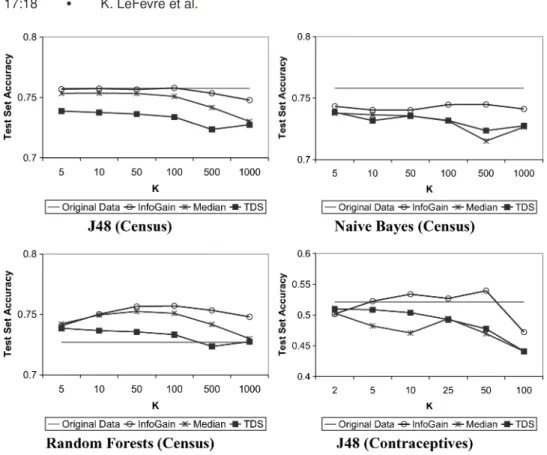
Fig. 7. Classification-based model evaluation using real-world data.
show test set accuracy (averaged across 10 folds) for three learning algorithms. The variance across the folds was quite low, and the differences between InfoGain Mondrian and TDS, and between InfoGain Mondrian and Median Mondrian, were highly significant based on paired t-tests.8
It is important to point out that in certain cases, notably Random Forests, the learning algorithm overfits the model when trained using the original data. For example, the model for the original data gets 97% accuracy on the training set but only 73% accuracy on the test set. When overfitting occurs, it is not surprising that the models trained on anonymized data obtain higher accu-racy because anonymization serves as a form of feature selection/construction. Interestingly, we also tried applying a traditional form of feature selection (ranked feature selection based on information gain) to the original data, and this did not improve the accuracy of Random Forests for any number of cho-sen attributes. We suspect that this discrepancy is due to the flexibility of the recoding techniques. Single-dimensional recoding (TDS) is more flexible than traditional feature selection because it can incorporate attributes at varying levels of granularity. Multidimensional recoding is more flexible still because it 8On the Census data, for J48 and Naive Bayes, when comparing InfoGain Mondrian vs. Median
Mondrian, and InfoGain Mondrian vs. TDS, the one-tailedp-value is always< .02 fork=5. For Random Forests, thep-value is< .02 fork=10.
Fig. 8. General-purpose quality measures using real-world data.
Fig. 9. Regression-based model evaluation using real-world data.
incorporates different attributes (at different levels of granularity) for different data subsets.
We performed the same set of experiments using the Contraceptives database and observed similar behavior. InfoGain Mondrian yielded higher accuracy than TDS or Median Mondrian. Results for J48 are shown in Figure 7.9
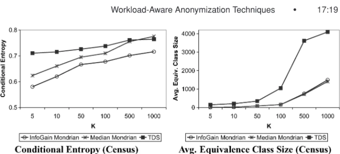
Next Figure 8 shows conditional entropy and average equivalence class-size measurements averaged across the ten anonymized training folds of the Census classification data. Notice that Median Mondrian and InfoGain Mondrian con-sistently produce equivalence classes of comparable size despite the difference in predictive accuracy; this indicates that average equivalence class size is not a very good indicator of data quality with respect to this particular workload. Conditional entropy, which incorporates the target class label, is better; low-conditional entropy generally indicates a higher-accuracy classification model. For regression, we found that Regression Mondrian generally led to better models than Median Mondrian. Figure 9(a) shows the mean absolute test set error for the M5 regression tree and a linear regression using the Census re-gression data.
9On the contraceptives data, when comparing InfoGain Mondrian vs. Median Mondrian and
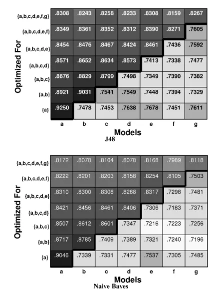
Fig. 10. Classification-based model evaluation for multiple models (k=25).
4.5 Multiple Target Models
In Section 3.1.2, we described a simple adaptation to the basic InfoGain Mon-drian algorithm that allowed us to incorporate more than one target attribute, expanding the set of models for which a particular anonymization is optimized. To evaluate this technique, we performed a set of experiments using the syn-thetic classification data, increasing the number of class labels.
Figure 10 shows average test set accuracies for J48 and Naive Bayes. We first generated 100 independent training and testing sets, containing 1,000 records each. We used synthetic labeling functions 2-6,7, and 9 from the Agrawal generator [Agrawal et al. 1993], randomly varying the constants in functions 2-6 as described in Section 4.4.
Each column in the figure (models A-G) represents the average of 25 random permutations of the synthetic functions. (i.e., to get a more robust result, we randomly re-ordered the class labels.) The anonymizations (rows in the figure) are optimized for an increasing number of target models. (e.g., the anonymiza-tion in the bottom row is optimized exclusively for model A.) There are two important things to note from the chart, and similar behavior was observed for the other classification algorithms.
— Looking at each model (column) individually, when the model is included in the anonymization (above the bold line), test set accuracy is higher than when the model is not included (below the line).
— As we increase the number of included models (moving upward above the line within each column), the test set accuracy tends to decrease. This is because the quality of the anonymization with respect to each individual model is diluted by incorporating additional models.
4.6 Privacy-Utility Trade off
In Section 3.1, we noted that there are certain cases where the trade off between privacy and utility is (more or less) explicit, provided that conditional entropy is a good indicator of classification accuracy. In particular, this occurs when the set of features is the same as the set of quasi-identifiers, and the sensitive attribute is the same as the class label or numeric target attribute.
In this section, we illustrate this empirically. Specifically, we conducted an experiment using entropy-diversity as the only anonymity requirement (i.e.,
k =1) for increasing values of parameter. We again used the Census classi-fication data, and this time let the salary class attribute be both the sensitive attribute and the class label. For eachvalue, we conducted an anonymization experiment, measuring the average conditional entropy of the resulting data (across the 10 folds) as well as the average test set classification accuracy.
The results are shown in Figure 11. As expected, the conditional entropy (across resulting partitions) increases for increasing.10Also, it is not surpris-ing that the classification accuracy slowly deteriorates with increassurpris-ing.
4.7 Selection
In Section 3.2, we discussed the importance of preserving selections and de-scribed an algorithm for incorporating rectangular selection predicates into an anonymization. We conducted an experiment using the synthetic data (1,000 generated records), but treating synthetic Function C2 as a selection pred-icate. Figure 12 shows the imprecision of this selection when evaluated us-ing the recoded data. The figure shows results for data recoded usus-ing three different anonymization algorithms. The first algorithm is Median Mondrian with greedy recursive splits chosen from among all of the quasi-identifier at-tributes. It also shows a restricted variation of Median Mondrian where splits 10When=1, the conditional entropy is greater than 0 due to a small number of records in the
Fig. 11. -Diversity experiment.
Fig. 13. Selection and projection experiment.
are made with respect to only Age and Salary. Finally, it shows the results of Selection Mondrian, incorporating Function C2 as three separate rectangular query regions (each with equal weight). It is intuitive that imprecision increases withk and that imprecision is reduced by incorporating the selection into the anonymization.
Incorporating selections can also affect model quality. In the absence of selec-tions, InfoGain and Regression Mondrian choose recursive splits using a greedy criterion driven by the target model(s). When selections are included, the re-sulting partitions may not be the same as those that would be chosen based on the target model(s). In the worst case, there may be a selection on an attribute that is uncorrelated with the target attribute.
To demonstrate this intuition, we performed an experiment using the Census classification data. To simulate the effect of selections that are uncorrelated with the target model, we first assigned each training tuple to one ofngroups, chosen uniformly at random. (We assume |Rn| ≥k.) We then anonymized each group independently, using either InfoGain Mondrian or Median Mondrian. Once recodings were determined for each training group, we randomly assigned each test tuple to one of thengroups and recoded the tuple using the recoding function for that group. Finally, we trained a single classification model using the full recoded training set (union of all training groups) and tested using the full recoded test set. This process was repeated for each of ten folds.
The results of this selection experiment for J48 are shown in Figure 13 for increasingnandk=50. As expected, accuracy decreases slightly as the num-ber of selections (n) increases. However, several selections can be incorporated without large negative effects. Similar results were observed for the other clas-sification algorithms.
4.8 Projection
In certain cases, the data recipient will not use all released attributes when con-structing a model. Instead, he or she will build the model using only a projected subset of attributes. In our experiments, we have found that single-dimensional recoding often preserves precise values for fewer attributes than does multidi-mensional recoding. (This was also observed in LeFevre et al. [2006a].)
In this section, we describe an experiment comparing anonymization algo-rithms when only a subset of the released features is used in constructing a particular model. In this experiment, we first ranked the set of all features us-ing the original data and a greedy information gain heuristic. We then removed the features in order, from most to least predictive, and constructed classifica-tion models using the remaining attributes. We fixedk=100.
As expected, test set accuracy decreases as the most predictive features are dropped. However, the rate of this decline varies depending on the anonymiza-tion algorithm used. Figure 13 shows the observed accuracies for J48 using the Census database. Because of the single-dimensional recoding pattern which preserves fewer attributes, this rate of decay is the most precipitous for TDS. The results were similar for the other classification algorithms and the Contra-ceptives data.
5. INCORPORATING SCALABILITY
While numerous anonymization algorithms have recently been proposed, few have considered datasets larger than main memory. Proposed scalable tech-niques [Mokbel et al. 2006; Iwuchukwu and Naughton 2007] based on spatial indexing do not support workload-oriented splitting heuristics. For this rea-son, we introduce and evaluate two external adaptations of the Mondrian al-gorithmic framework (Median Mondrian, InfoGain Mondrian, and Regression Mondrian). For clarity, we refer to the scalable variations asRothko.11
The first adaptation is based on ideas from the RainForest scalable decision tree algorithms [Gehrke et al. 1998]. Although the basic structure of the algo-rithm is similar to RainForest, there were several technical problems we had to address. First, in order to choose an allowable split (according to a given split criterion and anonymity requirement), we need to choose an appropriate set of count statistics since those used in RainForest are not always sufficient. Also, we note that in the anonymization problem, the resulting partition tree does not necessarily fit in memory, and we propose techniques addressing this problem.
The second adaptaion takes a different approach based on sampling. The main idea is to use a sample of the input datasetR(that fits in memory) and to build the partition tree optimistically according to the sample. Any split made in error is subsequently undone; thus, the output is guaranteed to satisfy all given anonymity requirements. We find that, for reasonably large sample sizes, this algorithm also generally results in a minimal partitioning.
5.1 Exhaustive Algorithm (Rothko-T)
Our first algorithm, which we callRothko-Tree(orRothko-T), leverages several ideas originally proposed as part of the RainForest scalable decision tree frame-work [Gehrke et al. 1998]. Like Mondrian, decision tree construction typically involves a greedy recursive partitioning of the domain (feature) space. For de-cision trees, Gehrke et al. [1998] observed that split attributes (and thresholds) 11Mark Rothko (1903-1970) was a Latvian-American painter whose late abstract expressionist
could be chosen using a set of count statistics, typically much smaller than the full input dataset.
In many cases, allowable splits can be chosen greedily in Mondrian using related count statistics, each of which is typically much smaller than the size of the input data.
—Median/k-Anonymity.Underk-anonymity and Median partitioning, the split attribute (and threshold) can be chosen using what we will call anAV group. TheAV setof attribute Afor tuple set R is the set of unique values of Ain
R, each paired with an integer indicating the number of times it appears in
R(i.e., SELECT A, COUNT(*) FROM R GROUP BY A). The AV group is the collection of AV sets, one per quasi-identifier attribute.
—InfoGain/k-Anonymity. When the split criterion is InfoGain, each AV set (group) must be additionally augmented with the class label, producing an AVC set (group) as described in Gehrke et al. [1998] (i.e., SELECT A, C, COUNT(*) FROM R GROUP BY A, C.).
—Median/-Diversity.In order to determine whether a candidate split is al-lowable under-diversity, we need to know the joint distribution of attribute values and sensitive values, for each candidate split attribute (i.e., SELECT A, S, COUNT(*) FROM R GROUP BY A, S). We call this the AVS set (group). —InfoGain/-Diversity.Finally, when the split criterion is InfoGain, and the anonymity constraint is -diversity, the allowable split yielding maximum information gain can be chosen using both the AVC and AVS groups.
Throughout the rest of the article, when the anonymity requirement and split criterion are clear from context, we will interchangeably refer to them as
frequency setsandfrequency groups.
When the anonymity requirement is variance diversity or the split criterion is Regression, the analogous summary counts (e.g., the joint distribution of attributeAand a numeric sensitive attributeSor numeric target attributeT) are likely to be prohibitively large. We return to this issue in Section 5.2.
In the remainder of this section, we describe a scalable algorithm for
k-anonymity and/or-diversity (using Median or InfoGain splitting) based on these summary counts. In each case, the output of the scalable algorithm is identical to the output of the corresponding in-memory algorithm.
5.1.1 Algorithm Overview. The recursive structure of Rothko-T follows that of Rain-Forest [Gehrke et al. 1998], and we assume that at least one fre-quency group will fit in memory. In the simplest case, the algorithm begins at the root of the partition tree and scans the input data (R) once to construct the frequency group. Using this, it chooses an allowable split attribute (and thresh-old) according to the given split criterion. Then, it scansRonce more and writes each tuple to a disk-resident child partition as designated by the chosen split. The algorithm proceeds recursively in a depth-first manner, dividing each of the resulting partitions (Ri) according to the same procedure.
Once the algorithm descends far enough into the partition tree, it will reach a point where the data in each leaf partition is small enough to fit in memory.
Fig. 14. Rothko-T example.
At this point, a sensible implementation loads each partition (individually) into memory and continues to apply the recursive procedure in memory.
When multiple frequency groups fit in memory, the simple algorithm can be improved to take better advantage of the available memory using an approach reminiscent of the RainForest hybrid algorithm. In this case, the algorithm first scansR, choosing the split attribute and threshold using the resulting fre-quency group. Now, suppose that there is enough memory available to (simulta-neously) hold the frequency groups for all child partitions. Rather than repar-titioning the data across the children, the algorithm proceeds in a breadth-first manner, scanningRonce again to create frequency groups for all of the children. Because the number of partitions grows exponentially as the algorithm de-scends in the tree, it will likely reach a level at which all frequency groups no longer fit in memory. At this point, it divides the tuples inRacross the leaves, writing these partitions to disk. The algorithm then proceeds by calling the pro-cedure recursively on each of the resulting partitions. Again, when each leaf partition fits in memory, a sensible implementation switches to the in-memory algorithm.
Example (Rothko-T). Consider input tuple set (R), and suppose there is enough memory available to hold 2 frequency groups forR. The initial execution of the algorithm is depicted in Figure 14.
Initially, the algorithm scans R once to create the frequency group for the root (1) and chooses the best allowable split (provided that one exists). (In this example, all of the splits are binary.) Then, the algorithm scans R once more to construct the frequency groups for the child nodes (2 and 3) and chooses the best allowable splits for these nodes.
Following this, the four frequency groups for the next level of the tree will not fit in memory so the data is divided into partitions R1,. . .,R4. The procedure is then called recursively on each of the resulting partitions.
5.1.2 Recoding Function Scalability. The previous section highlights an additional problem. Because the decision trees considered by Gehrke et al. [1998] were of approximately constant size, it was reasonable to assume that the resulting tree structure itself would fit in memory. Unfortunately, this is often not true of our problem.
Instead, we implemented a simple scalable technique for materializing the multidimensional recoding functionφ. Notice that each path from root to leaf in the partition tree defines a rule, and the set of all such rules defines global recoding functionφ. For example, in Figure 2, (Ag e < 40)∧(Nationality European)→ [0−40],Europeanis one such rule.
The set of recoding rules can be constructed in a scalable way, without fully materializing the tree. In the simplest case, when only one frequency group fits in memory, the algorithm works in a purely depth-first manner. At the end of each depth-first branch, we write the corresponding rule (the path from root to leaf) to disk. This simple technique guarantees that the amount of information stored in memory at any one time is proportional to the height of the tree, which grows only as a logarithmic function of the data.
When more memory is available for caching frequency groups, the amount of space is slightly larger due to the periods of breadth-first partitioning, but the approach still consumes much less space than materializing the entire tree.
Finally, note that the tree structure is only necessary if it is used to define a global recoding function that covers the domain space. If we instead choose to represent each resulting region using summary statistics, then the tree struc-ture need not be materialized. Instead, the summary statistics can be computed directly from the resulting data partitions.
5.2 Sampling Algorithm (Rothko-S)
In this section, we describe a second scalable algorithm, this time based on sampling. Rothko-Sampling (or Rothko-S) addresses some of the shortcomings of Rothko-T. Specifically, because splits are chosen using only memory-resident data, it provides us with the ability to choose split attributes using the Regres-sion split criterion and to check variance diversity. The sampling approach also often leads to better performance.
The main recursive procedure consists of three phases.
(1) (Optimistic)Growth Phase. The procedure begins by scanning input tuple setRto obtain a simple random sample (r) that fits in the available memory. (If R fits in memory, then r = R.) The procedure then grows the tree, using sampler to choose split attributes (thresholds). When evaluating a candidate split, it uses the sample to estimate certain characteristics of
R, and using these estimates, it will make a split (optimistically) if it can determine with high confidence that the split will not violate the anonymity requirement(s) when applied to the full partition R. The specifics of these tests are described in Section 5.2.1.
(2) Repartitioning Phase. Eventually, there will be no more splits that can be made with high confidence based on sampler. Ifr ⊂ R, then input tuple setRis divided across the leaves of the tree built during the growth phase. (3) Pruning Phase. When r ⊂ R, there is the possibility that certain splits were made in error during the growth phase. Given a reasonable testing procedure, this won’t happen often, but when a node in the partition tree is found to violate (one of) the anonymity requirement(s), then all of the
Fig. 15. Rothko-S example.
partitions in the subtree rooted at the parent of this node are merged. To do this, during the repartitioning phase, we maintain certain population statistics at each node. (Fork-anonymity, this is just a single integer count. For -diversity or variance diversity, we construct a frequency histogram over the set of unique sensitive values.)
Finally, the procedure is executed recursively on each resulting partition,
R1,. . .,Rm. In virtually all cases, the algorithm will eventually reach a base case where each recursive partition Ri fits entirely in memory. (There are a few pathological exceptions, which we describe in Section 5.2.2. These cases typically only arise when an extremely small amount of memory is available.)
Recoding function scalability can be implemented as described in Section 5.1.2. In certain cases, we stop the growth phase early for one of three possible reasons. First, if we are constructing a global recoding function and the tree structure has filled the available memory, we then write the appropriate recoding rules to disk. Similarly, we repartition the data if the statistics neces-sary for pruning (e.g., sensitive frequency histograms) no longer fit in memory. Finally, notice that repartitioning across a large number of leaves may lead to a substantial amount of nonsequential I/O if there is not enough memory available to adequately buffer writes. In order to prevent this from occurring, the algorithm may repartition the data while there still exist high-confidence allowable splits.
Example(Rothko-S). Consider an input tuple setR. The algorithm is depicted in Figure 15.