Are there common Mathematical Structures in Economics and Physics?
Jürgen Mimkes, Physics Department, Paderborn University, GermanyIntroduction
Economics is a field that looks into the future. We may know a few things ahead (ex ante), but most things we only know, afterwards (ex post). How can we work in a field, where much of the important information is missing? Mathematics gives two answers: 1. Probability theory leads to microeconomics: the Lagrange function optimizes utility under constraints of economic terms (like costs). The utility function is the entropy, the logarithm of probability. The optimal result is given by a probability distribution and an integrating factor.
2. Calculus leads to macroeconomics: In economics, we have two production factors, capital and labour. This requires two dimensional calculus with exact and not-exact differentials, which represent the “ex ante” and “ex post” terms of economics. An integrating factor turns a not-exact term (like income) into an exact term (entropy, the natural production function). The integrating factor is the same as in microeconomics and turns the not-exact field of economics into an exact physical science.
Complexity
Economics and social sciences are presently considered to be complexity sciences. Economic networks are generally interconnected in a complicated way, social interactions may sometimes even be hidden and very difficult to follow. In addition, no general basic theory exists and researchers are constructing their own models, without much relationship to others. Neoclassical theory stands next to game theory and heterogeneous agents. In this way a patchwork of economic and social rules is constructed with defects and little coherence. It may well be that this field is just a collection of experiences that are tied together by numerous stories. The field of economics may indeed be very complex, but complexity theory does not (yet?) exist! Indeed, many economists do not believe in a general theory of economics.
But if socio-economics is a science, there must be a general logic and a mathematical structure in this complex system! We may look at another complex system: the macro cosmos around us with galaxies and black holes, with neutron stars, suns and planets including our earth with rocks and plants and animals. And within this macro cosmos there is a micro cosmos of atoms and electrons, nuclei, quarks, bosons and many other particles. Surprisingly, this huge complex system follows six simple rules: Conservation of energy, momentum, angular momentum, charge, and light and heavy particle numbers. Would it be possible that social and economic systems have similar rules? This could be the solution to socio-economic complexity. But so far nobody has been able to find these rules. One possibility would be the application of the six rules of the macro- and micro cosmos to socio-economic systems. People and the economy are indeed part of the cosmos. And which rule should apply? All rules must apply, but only few will be affected by socio-economic systems. One could think of conservation of energy resources as a rule, as these resources play an important part in socio-economics: e. g. the chlorophyll process of
plants involves photons, electrons, CO2, O2, C atoms, molecules and energy. This would be the first indication that economics may indeed be a physical science. But the results are not sufficient to give an actual proof of equivalence of economics and physics.
Probability
The six laws of the macro- and micro cosmos are not the only way to formulate laws of a complex world. Economic and physical rules can only be valid, if they are probable. Accordingly, we may try to apply probability theory to complexity. A well-known approach is the Lagrange function L,
L (N) = K (N) + λ* ln P (N) → max! (1)
In mathematics P is called probability, K is the constraint and λ the integrating factor. The
functions L, K and P may be functions of the number N of elements of the system. A system will be in a stable and most probable state, if the Lagrange function L (N) is at extremum. This law may be applied to many sciences like physics, economics and social sciences:
In a children's playroom N toys may be stored in a special order. K (N) represents the order
of the toys in the playroom. The entropy ln P (N) is a measure of disorder of the toys. The integrating factor λ is the tolerance of disorder of the parents. After children start playing the chaos (ln P) in the playroom - according to Lagrange - will go to a maximum, if the parents tolerate disorder. In contrast, order (K) will only be at maximum, if the tolerance λ → 0, if the parents do not tolerate disorder at all: L (N) = K (N) → maximum!
In physics (L) or better (- L) is called free energy. The Lagrange equation is a principal law
of thermodynamics. The constraint K is the energy, the integrating factor λ is the mean energy or temperature of the physical system and ln P is called entropy. N is the number of atoms or molecules of the molecular system, which may be a solid, a liquid or a gas. The physical system will be stable, if the (negative) free energy is at maximum! Depending on the temperature the solid, the liquid or the gas will be the stable state of the molecules. Nearly all problems of thermodynamics, of chemistry, of metallurgy, of mechanical engineering, of meteorology and other fields of physical sciences may be solved by the Lagrange equation.
In economics the constraint K is the capital. The integrating factor λ is the mean capital or
standard of living and ln P is the utility function. In probability theory entropy ln P replaces the Cobb Douglas function as utility function. N is the number of laborers in the economic system, a company, a city or a country. All problems of economic optimization like minimization of costs may be solved by this Lagrange function. Every economic system is stable, if the Lagrange function is at extremum.
In social sciences the constraint K is given by the rules between N heterogeneous agents of a city or state, of a church, of a company, of a club or any other system. The rules may be traffic laws, civil laws, behavior, ethical conduct, customs or any other rules. The entropy ln P is the measure of disorder, disobedience, misconduct, sin or violation, and the integrating factor λ the tolerance of violations in the social system. At zero tolerance
the system will be in complete order. At growing tolerance the system will become disordered. Apparently, probability theory with constraints may be applied to socio- economic systems. The Lagrange function has nothing to do with physics, but the mathematical structure of the laws of economics and social science are the same as in physics. These results already demonstrate the equivalence of laws in economics and physics, as proposed by Mirowski.
Calculus 1: Riemann and Stokes Integrals
Investors would like to calculate the course of investments in advance like the flight of an arrow. Why is it not possible? Economic terms are divided into two categories: some economic terms like functions (F) can be calculated beforehand, ex ante, and others, like income (Y) can only be calculated afterwards, ex post. We can only file our income tax at the end of the year! Accordingly, the Solow model [3], the basis of economic growth, cannot be correct, income (Y) cannot be a function (F): ex ante cannot be equal to ex post! Y ≠ F (K, N). (2)
The solution to this problem is calculus in two dimensions, as economics depends on two production factors, capital and labor.
In calculus of one dimension only one integral exists, the Riemann integral. The integral depends on the limits A and B. This integral is generally known in social sciences. In calculus of two dimensions we have two integrals, the Riemann and the Stokes integral. Riemann integrals depend on the integral limits A and B and are path independent. Stokes integrals are path dependent, a different path of integration leads to a different result. Stokes integrals can only be calculated, after the path of integration is known. This
integral is generally not known to economists and social scientists.
A closed Riemann integral is always zero, the path from A to B is equal to the path from B to A. It is like walking around a ring. The integral value is predictable zero and corresponds to economic ex ante terms and to conservation laws.
A closed Stokes integral is never zero, the path from A to B is not equal to the path from B to A. The value of the integral is not predictable and corresponds to economic ex post terms. The value of the closed Stokes integral is either positive or negative, it is like walking along a spiral, up or down. The integral value of a Stokes integral is unpredictable and corresponds to economic ex post terms like income and profits. Economic output (Y) is a Stokes integral and depends on the way the product is produced [4].
There are many examples for closed Stokes integrals. In biology the blood circuit is a closed Stokes integral, the arteries carry carbon and oxygen and energy, the veins on the way back carry only carbon dioxide. In economics the monetary circuit of income and costs is a closed Stokes integral, as income and costs may not be equal, leading to growth or deficit. In physics the Carnot process of motors is a closed Stokes integral and leads growth or deficit of heat in heat pumps and refrigerators. In meteorology highs and lows are closed Stokes integrals winding up or down including hurricanes and tornados.
Magnetic fields are closed Stokes integrals winding in one or the other direction. Magnetic mean field theory is even applied to co-operating or competing societies. Again physical models may be applied to socio-economic systems, as both are based on the same mathematical structure.
Double entry accounting
In physical sciences every field has a certain natural basis: mechanics is ruled by Newton´s law, electrodynamics is governed by the Maxwell equations and thermodynamics by the first and second law. What would be the basic law of economics?
Every economy, every company has to do accounting, and the basis of all economic calculations is double entry accounting:
A household (H) works in industry (In) earning 100 € per day and spending 90 € for food and goods. The surplus is 10 € per day. This may be given by an excel calculation for the monetary and the productive circuit:
Monetary account + Productive account = 0
The sum of the monetary and the productive circuit is zero. We may write monetary and productive circuits as closed Stokes integrals:
∮ 𝜹 𝒀 + ∮ 𝜹 𝑳 = 0 (3)
The monetary circuit (δ Y) measures the productive circuit (δ L) in monetary units. This integral equation or double entry balance may be considered as the basic law of all economic transactions, and will lead to the laws of macro- and microeconomics.
Calculus 2: Exact and not exact differential forms
In calculus of two dimensions there are two types of differential forms: exact and not exact differentials. Exact differentials (d F) are integrated by Riemann integrals. They lead to functions (F) and correspond to ex ante terms in economics.
Not exact differentials (δ Y) are integrated by Stokes integrals and do not have a stem function (Y)! The not exact differential form corresponds to ex post terms in economics. The integral law of double entry accounting (3) may be written in differential forms [3]:
1. Law: δ Y = d K – δ L (4)
The 1. Law of eq. (4) is identical to the integral law in eq. (3). If we apply the closed integral to eq. (4), we obtain three closed integrals: the closed Stokes integrals of δ Y and δ L lead back to eq. (3), the closed Riemann integral of d K is zero!
The first law tells us that income (δ Y) is an ex post term and depends on capital (d K) and labor (δ L). This has been known before, but now it is written as a differential equation, like in natural science. The first law has been deducted from the double entry balance in eq. (3) and may be considered as the differential balance of all economic transactions. The second law is derived from calculus: a not exact differential form (δ Y) may be linked to an exact differential form (d F) by an integrating factor λ. The second law is the proof of the existence of an economic production function (F) and replaces the erratic Solow equation (2). Since economic terms are divided into ex ante and ex post terms, economic equation are now formulated by the corresponding exact and not exact differential forms. Thermodynamics
The laws of thermodynamics are given by the first and second law of thermodynamics:
1. Law: δ Q = d E – δ W (6)
2. Law: δ Q = T d S (7)
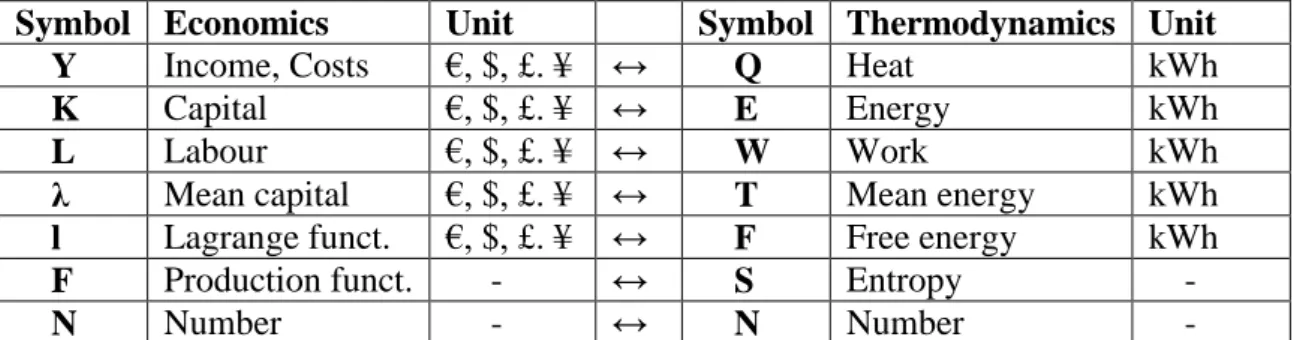
The first and second law of thermodynamics are applied to physics, chemistry, engineering and many other natural sciences. In addition, the structure of eqs. (6) and (7) is the same as in the first and second law of economics, eqs. (4) and (5). Only the dimensions differ: the laws of economics are calculated in monetary units like US $, €, £ or ¥, the laws of thermodynamics are measured in units of energy like J, kWh and kcal. However, due to the fixed oil price we may transform monetary units into energy units and vice versa. Accordingly, we may look at the law of thermodynamics as the laws of economics in energy units. This leads to an identity of economic and thermodynamic functions in table 1.
Symbol Economics Unit Symbol Thermodynamics Unit Y Income, Costs €, $, £. ¥ ↔ Q Heat kWh
K Capital €, $, £. ¥ ↔ E Energy kWh
L Labour €, $, £. ¥ ↔ W Work kWh
λ Mean capital €, $, £. ¥ ↔ T Mean energy kWh
l Lagrange funct. €, $, £. ¥ ↔ F Free energy kWh
F Production funct. - ↔ S Entropy -
N Number - ↔ N Number - Table 1. Corresponding terms in economics and thermodynamics.
Table 1 shows the corresponding terms of income (Y) and heat (Q), of capital (K) and energy (E), of labour (L) and physical work (W), of mean capital or standard of living (λ) and mean energy or temperature (T), of Lagrange function (l) and free energy (F), of production function (F) and entropy (S) etc.
The interpretation of the production function (F) by entropy (S) corresponds to eq. (1), where the utility function has been replaced by entropy S = ln P. Entropy leads economics to probability, as already discussed in the chapter on probability.
The Shannon entropy
S = ln P = N Σ i x i ln x i (8)
also leads to microeconomics, where (x i) represents the relative number of elements in the micro system: goods or commodities of different kind in a shop, or people like engineers, workers, secretaries, managers in a company, or industrial plants in an economy. Entropy is the most important function in economics, as has already been discussed by Georgescu-Roegen [1].
Conclusion
The question “Can economics be a physical science” leads to a positive answer, economics and natural sciences are equivalent, as already postulated in historical investigations by Mirowski. This result has now been discussed under aspects of modern natural science: general science, complexity, probability, calculus. As a result neoclassical theory has to be revised according to the first and second laws of thermodynamics. With Boltzmann´s interpretation of entropy economics and social sciences are closely connected to Thermodynamics, Lagrange equation and probability theory. Philip Mirkowski’s proposal holds: Economics is Social Physics and Physics is Nature´s Economics.
References
[1] Georgescu-Roegen, N., The Entropy Law and the Economic Process, Cambridge, Mass. Harvard Univ. Press, 1974
[2] Mirowski, P., More Heat than Light, Economics as Social Physics, Physics as Nature´s
Economics, Cambridge University Press (1989)
[3] Solow, A. R. M., Contribution to the Theory of Economic Growth, The Quarterly Journal of Economics, 70 (Feb. 1956) 65-94
[4] Mimkes, J., in Econophysics & Sociophysics: Trends & Perspectives, B. K. Chakrabarti, A. Chakraborti, A. Chatterjee (Eds.)