Performance Evaluation for Cost-Efficient Public
Infrastructure Cloud Use
John O’Loughlin and Lee Gillam Department of Computing, University of Surrey
Guildford, GU2 7XH, United Kingdom {john.oloughlin,l.gillam}@surrey.ac.uk
Abstract. In this paper, we discuss the nature of variability in compute perfor-mance in Infrastructure Clouds and how this presents opportunities for Cloud Service Brokers (CSB) in relation to pricing. Performance variation in virtual machines of the same type and price raises specific issues for end users : (i) the time taken to complete a task varies with performance, and therefore costs also vary (ii) the number of instances required to meet a certain problem scale within a given time being variable, so costs depend on variations in scale needed to meet the requirement; (iii) different computational requirements are better satis-fied by different hardware, and understanding the relationship between instance types and available resources implies further costs. We demonstrate such varia-bility problems empirically in a Public Infrastructure Cloud, and use the data gathered to discuss performance price issues, and how a CSB may re-price in-stances based on their performance.
Keywords: Infrastructure Clouds, Performance Variation, Simulation, Brokers
1
Introduction
Infrastructure as a Service (IaaS) Clouds are multi-tenant environments where re-sources such as networks, storage and servers are multiplexed between large numbers of users. The main characteristics of such systems include: self-provisioning of re-sources, on-demand acquisition, and the illusion of infinite scalability. Clouds are a metered service, so users are charged for the (units of) resources they consume per unit of time. The ability of the provider to allow users to acquire large scale resources at speed, and then release them when no longer needed, is referred to as elasticity.
The flexibility offered by Infrastructure Clouds makes their use popular for a varie-ty of purposes. However, a varievarie-ty of concerns have been raised regarding their use including, but not limited to: data security, privacy and sovereignty; service availabil-ity and the potential for provider failure; vendor lock in; and performance. The latter concern is primarily one of variation in the performance of instances that are suppos-edly of the same type, and results in a number of issues for users, including:
(i) prices are the same irrespective of performance, but costs will vary with the amount of time required to undertake a task;
(ii) as a consequence, when scaling an application the number of instances required to complete a certain amount of work in a given period of time may differ, and so the price for completing work is again variable;
(iii) different computational requirements will be better met by certain kinds of hardware which may be more attainable in a particular geographical location and, for a given user, determining the best value to task relationship in and across instance types across all geographies for a given Infrastructure Cloud im-plies further costs.
There is an opportunity for a Cloud Service Broker (CSB) to address these kinds of performance and cost related issues by being able to provide instances of known per-formance, and re-pricing them according to such performance levels. However, accu-rate performance simulations would be needed in order to derive a performance dis-tribution from which pricing schemes could, at minimum, encompass the costs of running a CSB, and beyond that to determine any profit margin. The priority for a CSB, then, is to obtain an accurate model of performance (variation).
In this paper we examine the issues that any such model of performance would need to consider. In particular, we show how performance is dependent on (1) loca-tion (2) account (3) workload and (4) VM allocaloca-tion polices. The rest of the paper is structured as follows: in Section 2 we discuss at some length the formulation of Clouds in terms of offerings, hardware, and geographies, the intricacies of which are essential to understand for any meaningful simulation. Section 3 offers a methodology for determining performance variation in Infrastructure Clouds, with results from an example set of performance variation evaluations in Section 4. Based on these results, Section 5 discusses the opportunities and challenges for a CSB, and discusses the factors that must be taken into account when modeling performance variation. Section 6 presents our conclusions and offers suggestions for future work in respect to pricing and CSBs.
2
Background
Infrastructure Clouds, such as Amazon's Elastic Compute Cloud (EC2), Google's Compute Engine (GCE) and the Rackspace Open Cloud, are typically structured into Regions and Availability Zones (AZs) [1]. Regions correspond to geographical areas, and their infrastructure is isolated from each other. Amazon’s EC2, for example, has 8 Regions in locations such as: North Virginia (us-east-1), Dublin (eu-west-1), and Sydney (ap-southeast-2).
Regions are physically comprised of multiple data centres, and these data centres are then structured into multiple AZs. From [2] we know that, as of 2012, the US-East-1 Region contained 10 data centres structured into 5 AZs. AZs power and net-work connections are independent of each other. The failure of one AZ should not, in theory, affect the operation of others in the same Region. In practice, failure cascade affecting multiple AZs has occurred on more than occasion, with one of the most
serious on June 29th 2012. Rackspace is a notable exception to the AZ model, stating that they guarantee 100% network availability [3] of the data centres which make up their Regions, and so claim there is no need to further expose the structure of the Re-gion.
Amazon also adopts a non-exposure principle: it is entirely possible that the same AZ identifier, such as us-east-1a, may map to different data centres for different ac-counts, perhaps even different network segments. Further, larger Regions, such as US East which has 5 AZs, restrict all new customers to just 3. Therefore different ac-counts are quite likely to have access to quite different locations within a Region. EC2 is further complicated by the fact that there are 2 different EC2 platforms: Classic-EC2 and Classic-EC2-VPC. The primary difference between them is the more advanced net-work features the latter provides. In a recent change, all new accounts will only have access to EC2-VPC.
Providers use virtualisation technologies atop specific hardware and the host oper-ating system, with Xen and KVM popular, to partition physical servers such that they can run one or more Virtual Machines (VMs). Each VM will be allocated one or more virtual CPUs (vCPUs), and the VM will be allocated CPU time via the hypervisor’s scheduling. A running VM is commonly referred to as an instance, and all Cloud Infrastructure providers should support requests for on-demand instances which can be started and terminated as needed. In addition to on-demand, EC2 also supports reserved instances and spot instances [4]. Reserved instances are more akin to tradi-tional hosting, purchased for either one year or three years, and require an up front payment that reserves the machine. In return, users are charged less per hour than for on-demand instances (depending on usage) and these can be turned on and off as required to avoid the additional usage costs - users are not charged additionally when the reserved instance is turned off. Spot instances make use of spare capacity but with unpredictability in availability. Indeed, price varies according to availability, and they can be reclaimed at any time without warning in order to support the higher value on-demand uses.
Instances are offered in a range of fixed sizes, know as instance types. Instance types typically specify some number of vCPUs, some amount of RAM, and some amount of local disk space. For example, an m1.medium instance on EC2 has 1 vCPU, 3.75GB of RAM and 410GB of local storage. Larger providers, such as EC2, GCE and HP, tend to group instance types into instance classes, also known as fami-lies. Instance types within the same instance class are typically ‘multiples’ of each other, for example, on EC2 the M1 class contains the m1.large, which has 2 vCPU, 7.5 GB of RAM and 820GB of local storage, so has twice the resources as the m1.medium, whilst the m1.xlarge has 4 vCPU, 15GB of RAM and 1640GB of local storage – and so is twice the m1.xlarge and quadruple the m1.medium. The price-per-hour scales similarly. Within a given instance class, the ratio of number of vCPUs to RAM is the same for all types, and for the M1 class this ratio is 3.75, and the compute power of a vCPU is the same across the whole class. As such, larger instance types are ‘more of the same’ as compared to smaller types in the class. EC2 offers a range of instance classes: General Purpose, High CPU, High Memory and High Storage.
Providers such as HP and GCE are following suit, albeit without any agreement on sizes.
Instance classes typically differ from each other in the following ways (1) ratio of vCPU to RAM (2) the amount of ‘compute power’ each vCPU in the class has (3) specialised hardware, such GPGPU cards and low latency networking. For (2), pro-viders have devised their own ratings for specifying the amount of ‘compute power’ that a vCPU will have. For example, EC2 has the EC2 Compute Unit (ECU), GCE has the Google Compute Engine Unit (GCEU) and HP Cloud use the HP Cloud Com-pute Unit (HPCCU). Provider supplied ratings are typically defined in terms of equiv-alence to specified hardware. As an example, GCE define a GCEU as: '…we choose 2.75 GCEUs to represent the minimum power of one logical core (a hardware hyper-thread) on our Sandy Bridge or Ivy Bridge platform'. These measures are typically used to express the expected relative performance of instances on the same Cloud, and so, on GCE, an instance with a vCPU core rated at 5.5 GCEUs should perform twice as well as one rated at 2.75 GCEUs. How these ratings are determined is not made public.
It is generally assumed that providers use a combination of 'weights' and 'limits' [5] to provide a guaranteed amount of CPU resources per vCPU. A weight indicates an amount of CPU time that the hypervisor should schedule for one vCPU relative to other vCPUs. For example, a vCPU with weight 100 will get half the CPU time as a vCPU with weight 200. As new VMs are started on hosts, and existing ones termi-nate, the number of vCPUs actually running on a host will fluctuate, so the amount of CPU resource per vCPU varies. Without a limit to both the number of vCPUs that can run on a host, and a maximum weight of vCPU, a minimum amount of CPU resource per vCPU cannot be guaranteed. With such limits are in place, providers can allocate a minimum amount of resources per vCPU. However, if the physical host is not at full capacity, i.e. the number of vCPUs running is less than the specified maximum, addi-tional CPU resources are available. Some providers let extant processes use spare cycles, and refer to ‘performance bursting’: a minimum CPU resource per vCPU is guaranteed but the vCPU can use any additional available capacity. Rackspace [6], in particular, allows for this, but given the difficulty in predicting when these extra re-sources will be available to a given VM it is hard to see how their use could be planned for in anything other than a statistical sense. Another option for managing spare CPU capacity is based on a CPU limit, which sets a maximum amount of CPU resource available per vCPU. If a limit is set above the minimum, some bursting is possible. This is a potential gain for the user but generates no income for the provider. If a limit is set at the minimum, an instance’s vCPUs has an amount of guaranteed CPU time but no more. From experimental data, as presented in section 4, EC2 ap-pears to operate this way. EC2 sells spare capacity as spot instances. This strategy appears beneficial to both user and EC2 – the user gets a consistent amount of CPU each time, and so making requirements planning easier, whilst the provider generates some income from otherwise unsold cycles.
Given the different characteristics of instance classes, it would seem that different hardware platforms are required to support different instance classes. This is certainly the case for specialised hardware such as GPGPU cards. However, even for classes
such as M2 High Memory and M1 General Purpose, there would appear to be 2 very good reasons for supporting these classes with their own hardware platforms: (1) VM allocation is simplified; (2) Hypervisor vCPU scheduling is simplified. For (1), the number of vCPU for a given instance type determines the RAM and local storage, so we need only find hosts that have a given vCPU capacity. By comparison, if we mix classes on hosts we need to find a host that has sufficient vCPU, RAM and local stor-age. For (2) we need only set the same weight and limit per vCPU for each instance type.
On EC2, it is readily possible to identify the CPU model types backing a particular instance. From this one can begin to associate platforms with instance classes - in-deed, for some instance classes this is advertised: the General Purpose M3 Class runs on Intel Xeon E5-2670 v2 (Sandy Bridge), the C3 High CPU Class runs on Intel Xeon E5-2680 v2 (Ivy Bridge) and the R3 High Memory Class runs on Intel Xeon E5-2670 (Ivy Bridge). Whilst the M3, C3 and R3, classes are currently associated with one hardware platform each, this is not the case for older instance classes. Indeed, the General Purpose M1 class is currently associated with at least 6. We have found, in addition to EC2, instance type heterogeneity exists on GoGrid, and also on Standard instance types from Rackspace. A number of papers have reported on performance variation on EC2, and some identify heterogeneity as the major cause: Armbrust et al. [15] describe EC2 performance as unpredictable; Osterman, et al. [16] describe per-formance in the Cloud as unreliable; Yelick, et al. [17] found that “applications in the Cloud…experience significant performance variations” and noted that this is in part caused by heterogeneity (of EC2); Phillips, Engen, and Papay [18] discovered differ-ential performance in instances of the same type on EC2 when attempting to predict application performance. In respect to Regions, Schad, et al. [19] showed that com-pute performance in US East N. California and EU West Dublin falls into two distinct performance bands which, upon further investigation breaks out by the two different CPU models backing their instances. Interestingly for our work, Ou, et al. [20], sug-gest that the heterogeneous nature of Clouds can be exploited by estimating the prob-ability of obtaining a particular CPU model backing an instance.
Understanding platform variation within an instance class, initially, is important because the compute performance of an instance is primarily determined by the plat-form it is running on. The time taken to complete an amount of work will depend on the hardware platform, and therefore the cost of completing the work also differs. We examine performance variation in detail in sections 3 and 4.
3
Experimental Setup
EC2 performance variations by CPU model have been widely reported on, as seen in the previous section. To produce valid simulations, we need to establish how perfor-mance varies by (1) location (2) account and (3) application. For the purpose of this paper, we explore the nature of running instances in all accessible AZs across 2 Re-gions (with respect to 1) using two different accounts (for 2) and a number of well known application-oriented benchmarks (3). Experiments were performed during
April and May 2014, with two EC2 accounts that we refer to as account A and ac-count B. We believe that Clouds inevitably become heterogeneous over time, and so the range of platforms backing a given instance class is also heterogeneous. We there-fore choose older Regions to see if this is supported: US-East-1, which is the original EC2 Region coming online in 2006, has 5 AZs, and is the default Region for requests if no Region is selected; and EU-West-1 which is the only European based Region at the time of writing, was the second Region to come online, in 2007, and offers 3 AZs.
Being financially constrained, we decided to use instances from the spot market. This gave us access to the same resources that both reserved and on-demand instances are sold from at reduced prices. As discussed, such instances can be reclaimed by EC2 when needed, and indeed this did happen to some of the instances run by account B before they were able to finish and report back results – as such, sample numbers may not be neatly rounded: we ended up with 350 instances for A, and 161 for B. Instances ran the official EC2 Precise Ubuntu AMIs supplied by Canonical (the ami-id differs by Region).
There are numerous metrics for compute performance that include floating point operations per second (FLOPs) and millions of instructions per second (MIPS). It is generally accepted that the performance metrics that are most useful and most in-formative to a user are: execution time and throughput [7][8]. Execution time is de-fined as the wall clock time for an application to execute, and is often referred to as application latency, and with hourly pricing for Infrastructure Clouds is a helpful measure for relating to costs. Where an application can be thought of as doing some specified unit of work, for example a file compression, an image rendering or a video transcoding, we define throughput, or application bandwidth, as the work done per unit of time. This metric allows users to relate amount of work done per unit of time to cost.
When measuring compute performance by application execution time or through-put, appropriate applications need to chosen. Applications which are CPU bound are generally good candidates, as the CPU is then the main factor in their performance. However, care must be taken in order to avoid common pitfalls. Small applications may fit into the CPU instruction cache and so their execution time will not be affected by access speeds associated with the various memory hierarchies. Difficulties in CPU comparability have led to a preference for so-called ‘real world’ benchmarks – CPU bound applications which are in common use, being run with realistic inputs. Such a preference is typified by the Standard Performance Evaluation Corporation (SPEC) benchmark suite [9], and we follow this approach to benchmarking.
In each of our instances, we run the following benchmarks in serial: Bzip2: File compression using ubuntu 10.04 ISO image for input
POV-Ray: Photo realistic ray tracing using the standard benchmark.pov for input GNUGO: The Go Game with test.sgf
NAMD: Bio molecular simulation using apoa1.namd STREAM: Memory bandwidth
The first 4 benchmarks are part of the SPEC 2006 benchmark suite, with bzip2 [10] and GNUGO [11] measuring integer performance, whilst POV-Ray [12] and NAMD
[13] measure floating point performance. For NAMD and POV-Ray we used the same input files as SPEC, however these were not available for bzip2 or GNUGO. The example input file for Go is freely available at the Go KGS homepage. STREAM [14] is a well known benchmark used for measuring memory bandwidth; the results re-ported here are for the triad kernel. The results of these experiments are described below.
4
Performance Variation
In this section, we present a selection of results chosen to illustrate the considerations that we believe are important, and that would need to be factored into any subsequent performance simulations.
4.1 Variation by CPU Model
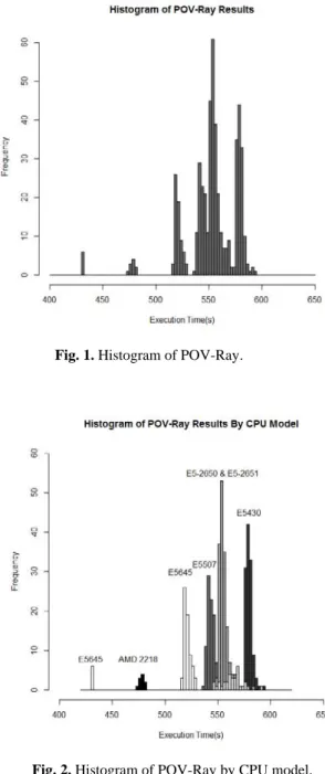
In Fig. 1, we present a histogram of the POV-Ray execution times, with an interval width of 2.5s. The histogram might be looked at as an emergent unimodal distribution with samples yet unseen at various intervals, but could also be seen as a multi-modal distribution. As discussed in section 2, we know that performance variation if often caused by differences in the CPU model underlying the instances, and we identified 6 different CPU models backing our instances: AMD 2281, Intel Xeon E5645, Intel Xeon E5507, Intel Xeon E5-2650, Intel Xeon E5-2651 and Intel Xeon E5430.
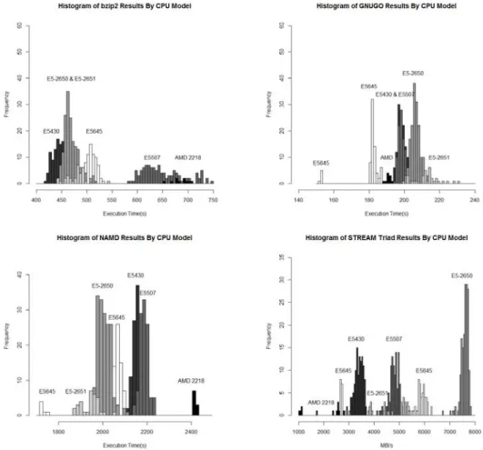
In Fig. 2, we present a histogram broken down by CPU model, and we see that the performance of POV-Ray is primarily determined by the CPU model the instance is running on, and there is little overlap in performance of the various CPU models, with the exception of the E5-2650 and E5-2561.
It is interesting to note that the very newest hardware platform in this set, the E5-2651 is outperformed by 4 of the older platforms. The AMD 2218 is a circa 2007 CPU model and outperforms all models here apart from an isolated number of E5645. It is often assumed that as Infrastructure Clouds introduce new platforms, these will outperform older generations, and such performance improvements will accrue to users without any increases in price. This is clearly not always the case.
Fig. 1. Histogram of POV-Ray.
4.2 Performance Variation by Application
POV-Ray results appear to depend on the CPU model, and here we have a best CPU model – the AMD 2218 (bar a few isolated E5645). It is natural to ask if we have identified a ‘best’ CPU model for all applications, and further, whether or not the ordering of CPU models by performance, is the same for different applications. Inter-estingly, this is not the case as the performance histograms for bzip2, GNUGO, NAMD and STREAM in Fig. 3 demonstrate, and so the relationship between CPU model and the nature of the application is important.
4.3 Performance Variation by Location
The physical composition of EC2 will evolve over time, for example as new Regions and AZs are added, and existing hardware is refreshed. As such, it is natural to ask if there are performance differences by location. Because identifiers such as us-east-1a potentially map to different locations for different accounts, we compare the mean results of the benchmarks across all these AZs for the instances for account A.
Table 1. Account A benchmark means across 5 AZs.
us-east-1a us-east-1c us-east-1d eu-west-1a eu-west 1b
POV-Ray(s) 559 551 569 519 558
Bzip2(s) 520 473 481 511 544
GNUGO(s) 196 203 198 184 198
NAMD(s) 2154 2009 2160 2104 2183
STREAM (MB/s) 4195 7268 3669 4253 3955
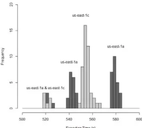
The percentage increase in mean execution time between the respective worst and best performing AZ is under 10% for POV-Ray, 15% for bzip2, and for STREAM the throughput difference is close to 100%. This would seem to support an argument that, with one or two exceptions, there is a little performance difference across AZs – and so no obvious advantage in choosing one over another. However, these numbers hide a lot of detail. The histogram below shows the POV-Ray results for east-1a and us-east-1c, which, from the table above, provide very similar mean performance.
We can see that both of these AZs have some overlap of instances which are perform-ing around 520s. AZ us-east-1a then has two levels of performance: one at just over 540s and one at 580s. Most instances in us-east-1c are performing around 550s. We can best understand this by looking the percentages of CPU models found in the us-east-1a and us-us-east-1a respectively.
Table 2. CPU model distribution
E5645 E5430 E5507 E-2650
us-east-1a 12% 50% 38% 0%
us-east-1c 12% 0% 0% 88%
Whilst mean performance is similar for both AZs, there does appear to be a strategy a user could adopt with us-east-1a to obtain better performance: keep instances backed by E5507, and throw away the E5430 instances – a deploy-and-ditch strategy. Over time, most instances would then perform at 545s or better. For us-east-1c, the only possibility for a similar strategy would be to keep E5645 and throw away E5-2650. With nearly 90% of the instances in this AZ backed by the E5-2650 this would clearly be much more expensive (the cost of an E5645-only strategy in us-east-1a would be a similar). Where performance consistency is important to a user, it is arguable that us-east-1c is better than us-east-1a.
4.4 Performance Variation By Account
As different accounts appear to have access to different AZs, obtainable performance can also differ by account. The accounts used in these experiments have mappings suggesting the following AZs in US-East-1 and EU-West-1:
Account A: us-east-1a, us-east-1c, us-east-1d, eu-west-1a, eu-west-1b and eu-west-1c Account B: us-east-1a, us-east-1b, us-east-1d, eu-west-1a, eu-west-1b and eu-west-1c
We compare performance for us-east-1a for both our accounts in Table 3:
Table 3. us-east-1a Account
POV-Ray(s)
Bzip2(s) GNUGO(s) NAMD(s) STREAM MB/s
A 559 520 196 2154 4195
B 551 469 205 2008 7342
For account A, there is an 11% increase in mean bzip2 execution time and 7% for NAMD. There is also a significant decrease in the memory bandwidth in A’s instanc-es as compared to B. Of the instancinstanc-es obtained by account B, 90% were backed by the E5-2650, and the remaining was E5645. Account A obtains a mix of E5430, E5645 and E5507 – but no E5-2650. It is possible that this is simply due to chance, and is a function of resource availability at the time of request. Another possibility is that
us-east-1a is a different location, and so a different set of resources, for both accounts. If this is the case, then for account B, performance will be consistent, but with no oppor-tunity for obtaining better performance than is offered by an E5-2650, whilst for ac-count A, such strategies are available.
5
Potential Opportunities for a CSB
Fixed prices for resources of the same type, together with a metered service, should offer users a consistent and predictable pricing for their Cloud usage. However, per-formance variation in instances of the same type results in variable and unpredictable costs. The absence of Service Level Agreements (SLAs) offering QoS terms with respect to compute performance presents an opportunity for a CSB who could deliver instances of known performance, at a price related to the performance. A CSB can exploit the fact that different CPU models are better, or worse, for different applica-tions, to provide a ‘match making’ service between a users application specific per-formance needs and available Cloud resources.
Whilst a user is of course free to engage in such work themselves, there is a cost in doing so, and this cost depends upon the various factors discussed in Section 4. Of course, there are also costs involved for a CSB. However, by dealing with a multiplic-ity of application needs (from perspective clients) over a larger range of Cloud re-sources a CSB is likely to be able make greater use of rere-sources obtained than an individual Cloud user. As such, the cost a CSB incurs in obtained instance of a de-sired performance level will, in general, be less than individual users. For example, a user wishing to run POV-Ray who obtains an instance backed by a E5430 may well look to ‘ditch’ this instance in favor of obtaining another CPU model. However, a CSB would view this instance as very good for bzip2 and reasonable for GNUGO.
Such a service could be advantageous to users in the following ways: (1) it offers better performance than a user may be able to obtain themselves; (2) it eliminates the variation due to differing resources (CPUs) being obtained; (3) it provides the re-quired performance when the user requires it, so offers performance on-demand. Of course, determining appropriate pricing schemes is now crucial, for both incentivizing users and allowing the CSB to run at a profit. Consequently, developing simulations of performance pricing are needed, and in turn this requires using a realistic model of how Clouds currently works - one which takes into account that performance varia-tion is a factor of (1) CPU model, (2) applicavaria-tion, (3) locavaria-tion, (4) account.
6
Conclusions and Future Work
In this paper, we have discussed the nature of variability in performance in Infrastruc-ture Clouds and how this presents opportunities for Cloud Service Brokers (CSB) in relation to pricing. We have shown that performance variation exists in various ways, for machine instances purportedly offering the same capability, across geographical regions and zones, across user accounts, and most importantly across heterogeneous hardware backing machine instances, and identified the kinds of issues that this raises
for end users. Further, we have demonstrated how such variability problems present in a real Public Infrastructure Cloud and how these can be application-specific.
From the data gathered from our experiments, we have been able to suggest how performance variation could be simulated such that a CSB could consider strategies for usefully re-pricing instances based on their performance in order to ensure profit-ability. The next step for this work is to use such a formulation and develop and eval-uate the simulation.
References
1. Regions, http://docs.aws.amazon.com/AWSEC2/latest/UserGuide/using-regions-availability-zones.html
2. AWS Service Event, http://aws.amazon.com/message/67457/
3. Rackspace Datacenters, http://www.rackspace.com/about/datacenters/ 4. EC2 Purchasing Options, http://aws.amazon.com/ec2/purchasing-options/ 5. Xen Credit Scheduler, http://wiki.xen.org/wiki/Credit_Scheduler
6. Rackspace Performance Cloud Servers, http://www.rackspace.com/knowledge_ center/article/what-is-new-with-performance-cloud-servers
7. D. Lilja: Measuring Computer Performance, New York, Cambridge University Press, (2000)
8. J. Hennessy and D. Patterson: Computer Architecture a Quantitative Approach, 5th Ed. Waltham, Elsevier, (2012)
9. Standard Performance Evaluation Corporation, http://www.spec.org 10. Bzip2, http://www.bzip.org
11. GNU Go, http://www.gnugo.org
12. Persistence of Vision, http://www.povray.org
13. NAMD Scalable Molecular Dynamics, http://www.ks.uiuc.edu/Research/namd/ 14. STREAM, Sustainable Memory Bandwidth in High Performance Computers,
http://www.cs.virginia.edu/stream/
15. M. Armbrust, A. Fox, R. Griffith, A.D. Joseph, R.H. Katz, A. Konwinski, G. Lee, D.A. Patterson, A. Rabkin, I. Stoica & M. Zaharia: Above the clouds: a Berkeley view of cloud computing, Technical Report EECS-2008-28, EECS Department, University of Califor-nia, Berkeley (2009).
16. S. Osterman, A. Iosup, N. Yigitbasi, R. Prodan, T. Fahringer, D. Epema: A performance analysis of EC2 cloud computing services for scientific computing, Cloud Computing, Lecture Notes of the Institute for Computer Sciences, Social-Informatics and Telecommu-nications Engineering, vol 34, pp 115-131 (2010).
17. K. Yelick, S. Coghlan, B. Draney, R.S. Canon: The Magellan Report on Cloud Computing for Science, http://www/alcf.anl.gov/magellan (2011).
18. S. Phillips, V. Engen, V., & J. Papay: Snow white clouds and the seven dwarfs, in Proc. of the IEEE International Conference and Workshops on Cloud Computing Technology and Science, pp738-745 (2011).
19. J. Schad, J. Dittrich, and J.-A. Quiane-Ruiz, “Runtime measurements in ´the cloud: Ob-serving, analyzing, and reducing variance,” Proc. VLDB Endow., vol. 3, no. 1-2, pp. 460– 471 (2010).
20. Ou, Z., et al,.: Exploiting Hardware Heterogeneity within the same instance type of Ama-zon EC2, presented at 4th USENIX Workshop on Hot Topics inCloud Computing, Boston, MA. (2012).