Denoising of Medical Images Using Dual Tree Complex Wavelet Transform

(1)

Procedia Technology 4 ( 2012 ) 238 – 244

C3IT-2012

Denoising of medical images using dual tree complex

wavelet transform

V Naga Prudhvi Raj

a

, Dr T Venkateswarlu

b

a_{Associate Professor,Dept. of EIE, VR Siddhartha Engineering College, Vijayawada, 520007, India} b_{Professor, University College of Engineering, Sri Venkateswara University, Tirupati, India}

Abstract

In Medical diagnosis operations such as feature extraction and object recognition will play the key role. These tasks will become difficult if the images are corrupted with noise. So the development of effective algorithms for noise removal became an important research area in present days. Developing Image denoising algorithms is a difficult task since fine details in a medical image embedding diagnostic information should not be destroyed during noise removal. Many of the wavelet based denoising algorithms use DWT (Discrete Wavelet Transform) in the decomposition stage are suffering from shift variance and lack of directionality. To overcome this in this paper we are proposing the denoising method which uses dual tree complex wavelet transform to decompose the image and shrinkage operation to eliminate the noise from the noisy image. In the shrinkage step we used semi-soft and stein thresholding operators along with traditional hard and soft thresholding operators and verified the suitability of dual tree complex wavelet transform for the denoising of medical images. The results proved that the denoised image using DTCWT (Dual Tree Complex Wavelet Transform) have a better balance between smoothness and accuracy than the DWT and less redundant than UDWT (Undecimated Wavelet Transform). We used the SSIM (Structural similarity index measure) along with PSNR (Peak signal to noise ratio) to assess the quality of denoised images.

Keywords: Discrete Wavelet Transform; Undecimated Wavelet Transform; Wavelet Shrinkage; Dual Tree Complex Wavelet Transform.

1. Introduction

Medical information, composed of clinical data, images and other physiological signals, has become an essential part of a patient’s care, whether during screening, the diagnostic stage or the treatment phase. Over the past three decades, rapid developments in information technology (IT) & Medical Instrumentation has facilitated the development of digital medical imaging. This development has mainly concerned Computed Tomography (CT), Magnetic Resonance Imaging (MRI), the different digital radiological processes for vascular, cardiovascular and contrast imaging, mammography, diagnostic ultrasound imaging, nuclear medical imaging with Single Photon Emission Computed Tomography (SPECT) and Positron Emission Tomography (PET). All these processes are producing

Open access under CC BY-NC-ND license.

(2)

ever-increasing quantities of images. These images are different from typical photographic images primarily because they reveal internal anatomy as opposed to an image of surfaces [11].

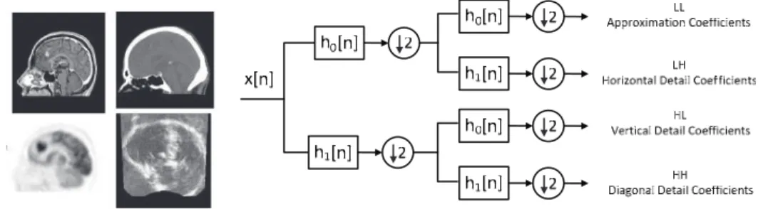
In Natural monochromatic or colour images, the pixel intensity of the image corresponds to the reflection coefficient of natural light. Whereas images acquired for clinical procedures reflect very complex physical and physiological phenomena, of many different types, hence the wide variety of images [11]. Each medical imaging modality (digital radiology, computerized tomography (CT), magnetic resonance imaging (MRI), ultrasound imaging (US)) has its own specific features corresponding to the physical and physiological phenomena studied, as shown in “Fig.1”. These medical mages have their own unique set of challenges. Although our focus in this paper will be on two-dimensional images, three-dimensional (volume) images, time-varying two-dimensional images (movies), and time-varying three-dimensional images are commonly used clinically as imaging modalities are becoming more sophisticated [11].

Fig. 1. (a) Sagittal slices of the brain by different imaging modalities; (b) 2D DWT single stage decomposition

(c) 2D DWT Multi stage decomposition

Spatial filters are traditional means of removing noise from images and signals [11]. Spatial filters usually smooth the data to reduce the noise, and also blur the data. Several new techniques have been developed in the last few years that improve on spatial filters by removing the noise more effectively while preserving the edges in the data. Some of these techniques used the ideas from partial differential equations and computational fluid dynamics such as level set methods, total variation methods [1], non-linear isotropic and anisotropic diffusion, Other techniques combine impulse removal filters with local adaptive filtering in the transform domain to remove not only white and mixed noise, but also their mixtures [11][3]. In order to reduce the noise present in medical images many techniques are available like digital filters (FIR or IIR), adaptive filtering methods etc. However, digital filters and adaptive methods can be applied to signal whose statistical characteristics are stationary in many cases. Recently the wavelet transform has been proven to be useful tool for non-stationary signal analysis [3][7]. Many denoising algorithms were developed on wavelet framework effectively but they suffer from four shortcomings such as oscillations, shift variance, aliasing, and lack of directionality. In this paper we will present a different class of methods which exploits the decomposition of the data into the dual tree complex wavelet basis and shrinks the wavelet coefficients in order to denoise the data [6],[7],[3].

LH1

HL1 HH1 LH2

HL2 HH2 LL2

(3)

While this is typically done using the more memory efficient decimated wavelet transforms, the use of non-decimated transforms will minimize the artifacts in the denoised data [7].

2. Dual tree complex wavelet transform

The dual tree complex wavelet transform is directionally selective and shift invariant in two and higher dimensions. The dual tree complex wavelet transform introduces the redundancy by a factor of

2

d_for

_d

dimensions which is lower than the redundancy introduced by UDWT (Undecimated

Wavelet Transform) [7]. Since last 20 years DWT (Discrete Wavelet Transform) has proven excellent tool for analysis of one dimensional signal’s by replacing the Fourier Transform’s infinitely oscillating sinusoidal basis functions with a set of locally oscillating functions called wavelets. But its performance is poor in the analysis of complex and modulated signals such as radar, speech, music, higher dimensional medical and geophysics data. In these areas the complex wavelet transform will give a better performance than critically sampled DWT.

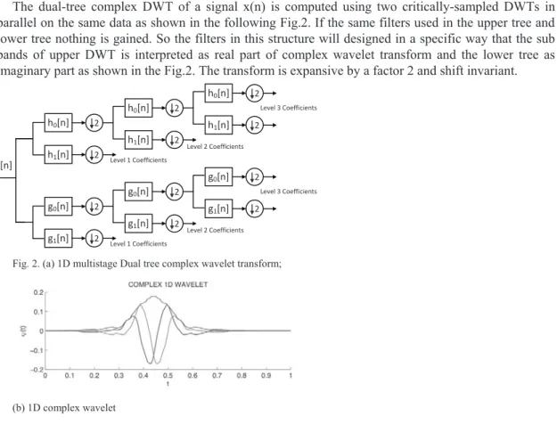
The dual-tree complex DWT of a signal x(n) is computed using two critically-sampled DWTs in parallel on the same data as shown in the following Fig.2. If the same filters used in the upper tree and lower tree nothing is gained. So the filters in this structure will designed in a specific way that the sub bands of upper DWT is interpreted as real part of complex wavelet transform and the lower tree as imaginary part as shown in the Fig.2. The transform is expansive by a factor 2 and shift invariant.

Fig. 2. (a) 1D multistage Dual tree complex wavelet transform;

(b) 1D complex wavelet

There are various methods to design the filters for dual tree complex wavelet transform. The detailed study of filter design is found in the article “The Dual-Tree Complex Wavelet Transform” by Nick G. Kingsbury [2]. The filters must satisfy the desired properties such as approximate half sample property, Perfect Reconstruction (Orthogonal or Biorthogonal), Finite support (FIR filters), and Vanishing moments/good stop band, Linear phase [2].

3. Denoising algorithm

The wavelet shrinkage is a signal denoising technique based on the idea of thresholding the wavelet coefficients. Wavelet coefficients having small absolute value are considered to encode mostly noise and very fine details of the signal. In contrast, the important information is encoded by the coefficients

h0[n] 2 h1[n] 2 h0[n] 2 h1[n] 2 h0[n] 2 h1[n] 2 Level 1 Coefficients Level 2 Coefficients Level 3 Coefficients g0[n] 2 g1[n] 2 g0[n] 2 g1[n] 2 g0[n] 2 g1[n] 2 Level 1 Coefficients Level 2 Coefficients Level 3 Coefficients x[n]

(4)

having large absolute value. Removing the small absolute value coefficients and then reconstructing the signal should produce signal with lesser amount of noise. The wavelet shrinkage approach can be summarized as follows [3], [4], [5], [6], [9]:

Consider the standard univariate non-parametric regression setting

( )

( ) for

1, 2,...,

i i i

X t

S t

V

N t

i

m

(1)

Where

X t

_i

( )

’s are assumed to come from Zero-Mean normal distribution,

N t

_i

( )

’s are independent

standard normal N(0,1) random variables and noise level

' '

V

may be known or unknown. The goal is

to recover the underlying function ‘S’ from the noisy data,’ X’ without assuming any particular parametric structure for ‘S’.

1. Calculate the wavelet coefficient matrix’ w’ by applying a wavelet transform ‘W’ to the data

( )

(

)

w W X

W S

W

V

N

(2)

2. Modify the detail coefficients of w to obtain the estimate

w

ˆ

of the wavelet coefficients of S.

ˆ

w

o

w

(3)

3. Inverse transform the modified detail coefficients to obtain the denoised coefficients.

1

ˆ

_{( )}

_ˆ

S W

w

₍₄₎

Thresholding methods can be grouped into two categories, global thresholds and level dependent thresholds. The former method chooses a single value for threshold T to be applied globally to all empirical wavelet coefficients while the later method uses different thresholds for different levels. In

this work we have used the universal threshold, which is a simple entropy measure totally depends on

the size of the signal: T = ı.sqrt(2*log(K)), where K is the size of the signal and T is the threshold

value. These thresholds require an estimate of the noise level

' '

V

.The usual standard deviation of the

data values is clearly not a good estimator, unless the underlying function ‘S’ is reasonably flat. Donoho

and Jhonstone considered estimating

' '

V

in the wavelet domain and suggested a robust estimate that is

based only on the empirical wavelet coefficients at the finest resolution level. The reason for considering only the finest level is that the corresponding empirical wavelet coefficients tend to consist mostly of noise. Since there is some signal present even at this level, Donoho and Jhonstone proposed a

robust estimate of the noise level

' '

V

(based on the (MAD) median absolute deviation) given by

Here w0, w1, etc... are detail coefficients at the finest level.

Shrinkage step: Let

' '

w

denote a single detail coefficient and

' '

w

ˆ

denote its shrink version. Let ‘T’

be the threshold and

D

T

(.)

denote the shrinkage function which determines how threshold is applied to

the data and

' '

V

ˆ

be the estimate of the standard deviation

' '

V

of the noise in Eq (1). Then

(5)

By dividing

' '

w

with

' '

V

ˆ

we standardise the

' '

w

coefficients to get

'

w

_s

'

and to this standardised

'

w

s

'

we apply the threshold operator. After thresholding the resultant coefficients are multiplied

: 1, 2,... 2 ˆ ( ) 0.6745 j k median w j mad V ½ ® ¾ ¯ ¿

ˆ

ˆ.

ˆ

T

w

V

D

V

§

· ¨

¸

©

¹

(5)

with

' '

V

ˆ

to obtain

' '

w

ˆ

. If

' '

V

ˆ

is built into the Thresholding model or if the data is normalised with

respect to noise standard deviation, equation for estimated value of

' '

w

is

ˆ

T

w D w

(6)

Another open question in the wavelet shrinkage algorithm is how to apply the threshold. The

so-called hard thresholding method zeros the coefficients that are smaller than the threshold and leaves the

other ones unchanged. In contrast, the soft thresholding scales the remaining coefficients in order to

form a continuous distribution of the coefficients centered on zero. Several varieties of soft thresholding

are described in the literature [3][4][6][7]. In our experiments we have used four thresholding techniques. They are Hard Thresholding, Soft Thresholding, Semi-Soft Thresholding, and Stein Thresholding and compared their efficiency of denoising the medical images based on PSNR (Peak Signal to Noise Ratio).

Table 1. Various thresholding operators

Hard Thresholding Soft Thresholding Semi-soft Thresholding

for all ( ) 0 T H w w D w otherwise ! ® ¯

( ) sgn( ) max 0;

s H

D w

w

w T

1 0 1 ( ) sgn( ) 1 TT SS w T w T D w w T w T T w w d ° ° ® ° ! ° ¯

Semi-soft thresholding is a family of non-linearity’s that interpolates between soft and hard thresholding. It uses both a main threshold T and a secondary threshold T1=mu*T. When mu=1, the semi-soft thresholding performs a hard thresholding, whereas when mu=infinity, it performs a soft thresholding.

Stein Thresholding: Another way to achieve a trade-off between hard and soft thresholding is to use a soft-squared thresholding non-linearity, also named a Stein estimator.

4. Results & Conclusions

In this paper we used the Universal threshold and applied it globally. We used MAD method to estimate the noise level. For DWT and UDWT based denoising we used ‘dB4’ and symlet family wavelets. Finally we used the Hard, Soft, Semi-soft, and Stein Thresholding functions for the shrinkage of wavelet coefficients and compared their efficiency of denoising the images based on PSNR (Peak Signal to Noise Ratio) and SSIM (Structural Similarity Index measure).

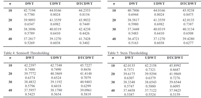
The tabulations were made ı vs PSNR

and

SSIM for DWT, UDWT and Dual Tree Complex

wavelets and four shrinkage functions as shown in the following tables. If the PSNR value is high it does not mean that the image is denoised in better way. Even the noise is removed it suffers from blurring and ringing effects when DWT is used. These artifacts are eliminated by using Dual tree Complex Wavelet Transform in place of DWT. The denoised images were shown in the Fig.3.

(6)

Table2: Hard Thresholding

Table 3: Soft Thresholding

ı DWT UDWT DTCDWT 10 42.7194 0.7780 44.0166 0.8024 44.2353 0.8154 20 39.9093 0.6547 41.3559 0.6982 43.9032 0.7449 30 38.3896 0.5789 40.0319 0.6410 42.4238 0.4426 40 37.2817 0.5269 39.1270 0.6038 41.7428 0.3402 ı DWT UDWT DTCDWT 10 40.7806 0.6944 44.0166 0.8024 45.9238 0.8475 20 38.5817 0.5980 41.3559 0.6982 42.0135 0.7387 30 37.3448 0.5483 40.0319 0.6410 40.3134 0.6508 40 36.4721 0.5163 37.1270 0.6038 39.4280 0.6277

Table 4: Semisoft Thresholding Table 5: Stein Thresholding

ı DWT UDWT DTCDWT 10 42.2397 0.7480 42.7348 0.7490 45.7227 0.8656 20 39.7772 0.6374 40.3869 0.6524 41.4148 0.7079 30 38.4832 0.5796 39.1192 0.6018 40.9403 0.6299 40 37.5957 0.5425 38.1780 0.5654 39.0961 0.5819 ı DWT UDWT DTCDWT 10 42.0135 0.7371 42.2158 0.7321 45.8992 0.8687 20 39.6175 0.6307 39.9294 0.6379 41.9869 0.7276 30 38.3348 0.5747 38.6543 0.5880 39.6544 0.6095 40 37.4458 0.5387 37.7122 0.5524 37.9425 0.5159

PSNR (Peak Signal to Noise Ratio)

PSNR is the peak signal-to-noise ratio in decibels (dB). The PSNR is only meaningful for data encoded in terms of bits per sample, or bits per pixel. For example, an image with 8 bits per pixel contains integers from 0 to 255.

(7)

The structural similarity (SSIM) index is a method for measuring the similarity between two images [8]. The SSIM index is a full reference metric, in other words, the measuring of image quality based on an initial uncompressed or distortion-free image as reference. SSIM is designed to improve on traditional methods like peak signal-to-noise ratio (PSNR) and mean squared error (MSE), which have proved to be inconsistent with human eye perception [8]. The SSIM metric is calculated on various

windows of an image. The measure between two windows x and y of common size N×N is :

(8)

Where

P

_x

the average of

' '

x

and

P

y

the average of

' '

y

x

V

_x2 the variance of

' '

x

and

V

_y2the variance of

' '

y

,

x

V

_xy the covariance of

' '

x

and

' '

y

,

x

c

₁

k L

₁

2,

c

₂

k L

₂

2, two variables to stabilize the division with weak denominator,

L the dynamic range of the pixel-values (typically this is

2

#bits per pixel

1

),

k

₁

0.01

and

2

0.03 k

by default. 10 2 1 20log B PSNR MSE § · ¨ ¸ © ¹

1 2 2 2 2 2 1 2 2 2 ( , ) x y xy x y x y c c SSIM x y c c P P V P P V V

(7)

Fig.3. (a) Original Image; (b) Image corrupted with noise; (c) Denoised image by DWT; (d) Denoised image by UDWT; (e) Denoised Image by DTCWT

From the above results it is found that the dual tree complex wavelet transform is outperforming in Denoising procedures without losing the useful information such as edges and textures with minimum amount of redundancy.

References

1. Yang Wang and Haomin Zhou, “Total Variation Wavelet-Based Medical Image Denoising”, International Journal of Biomedical Imaging, Hindawi Publication, Volume 2006 Article ID89095, pages 1-6, 2006.

2. Ivan W.Selesnick, Richard G.Baraniuk, Nick G. Kingsbury, “The Dual Tree Complex Wavelet Transform”, IEEE Signal Processing Magazine, November 2005.

3. Stephane Mallat, “A Wavelet Tour of signal Processing”, Elsevier, 2006.

4. D L Donoho and M. Jhonstone, “Wavelet shrinkage: Asymptopia? ”, J.Roy.Stat.Soc., SerB, Vol.57, pp. 301-369, 1995. 5. K.P Soman, K.I.Ramachandran, “Insight into Wavelets From theory to practice”, Prentice Hall India, 2004.

6. D L Donoho, “De-Noising by Soft-Thresholding”, IEEE Transactions on Information Theory, vol.41, No.3, May 1995. 7. Imola K. Fodor, Chandrika Kamath, “Denoising through wavlet shrinkage: An empirical study”, Center for applied

computing Lawrence Livermore National Laboratory, July 27, 2001.

8. Z. Wang, A. C. Bovik, H. R. Sheikh and E. P. Simoncelli, "Image quality assessment: From error visibility to structural similarity," IEEE Transactions on Image Processing, vol. 13, no. 4, pp. 600-612, Apr. 2004.

9. V N Prudhvi Raj, Dr T Venkateswarlu, “ECG Signal denoising using undecimated wavelet transfrom”, ICECT2011, Kanyakumari, India.

10. I.Daubechies, “Ten Lectures on Wavelets”, SIAM Publishers, 1992. 11. Rangaraj.M.Rangayyan, “Biomedical Image Analysis”, CRC press, 2005.

Original Image 50 100 150 200 250 50 100 150 200 250

Noisy Image (sigma=10)

50 100 150 200 250 50 100 150 200 250