Parameter estimation of breast tumour using
dynamic neural network from thermal pattern
Elham Saniei
a, Saeed Setayeshi
a,*
, Mohammad Esmaeil Akbari
b, Mitra Navid
ca
Energy Engineering and Physics Faculty, Amirkabir University of Technology, Tehran, Iran
b
Cancer Research Center, Shahid Beheshti University of Medical Sciences, Tehran, Iran
c
Medical Thermography Dept., Fanavaran Madoon Ghermez Co. Ltd., Tehran, Iran
G R A P H I C A L A B S T R A C T
Block diagram of the proposed model and Schema of applied dynamic neural network.
A R T I C L E I N F O Article history:
Received 9 February 2016
Received in revised form 27 May 2016 Accepted 29 May 2016
Available online 3 June 2016
Keywords:
Breast tumour
A B S T R A C T
This article presents a new approach for estimating the depth, size, and metabolic heat genera-tion rate of a tumour. For this purpose, the surface temperature distribugenera-tion of a breast thermal image and the dynamic neural network was used. The research consisted of two steps: forward and inverse. For the forward section, a finite element model was created. The Pennes bio-heat equation was solved to find surface and depth temperature distributions. Data from the analy-sis, then, were used to train the dynamic neural network model (DNN). Results from the DNN training/testing confirmed those of the finite element model. For the inverse section, the trained neural network was applied to estimate the depth temperature distribution (tumour position) * Corresponding author at: Tel.: +98 (21) 64540.
E-mail address:[email protected](S. Setayeshi). Peer review under responsibility of Cairo University.
Production and hosting by Elsevier
http://dx.doi.org/10.1016/j.jare.2016.05.005
2090-1232Ó2016 Production and hosting by Elsevier B.V. on behalf of Cairo University.
Neural network Thermal pattern Finite element model Pennes bio-heat equation Image
from the surface temperature profile, extracted from the thermal image. Finally, tumour param-eters were obtained from the depth temperature distribution. Experimental findings (20 patients) were promising in terms of the model’s potential for retrieving tumour parameters.
Ó2016 Production and hosting by Elsevier B.V. on behalf of Cairo University. This is an open access article under the CC BY-NC-ND license (http://creativecommons.org/licenses/by-nc-nd/ 4.0/).
Introduction
Breast cancer is the most common type of cancer in the world and survival chances vary by stage at diagnosis [1]. In risk assessment of patients suspected of having breast cancer, ther-mography plays a key role. Breast therther-mography is a valuable method for cancer diagnosis in early stages of tumour growth, when it is not yet recognizable by mammography. Patients with an abnormal thermogram have a high risk of developing breast cancer during their lifetime [2,3]. Thermography is a physiological test while mammography is an anatomical one
[3]. Thermovision techniques have been widely used to detect malignant breast tumours[4].
One basic question for breast thermography is how to quantify complex relationships between breast thermal pat-terns and underlying heat source parameters (size, depth and metabolic heat generation rate)[5]. Similar to other inverse problem applications, solving the breast thermography inverse problem is typically much more challenging, compared to its forward counterpart because of its intrinsically ill-posed nature.
Many researches have been conducted to understand rela-tionships between surface thermal patterns and underlying physiological or pathological parameters. Analysing surface temperature and tissue temperature profiles, Ng and Sud-harsan developed a 3-D direct numerical model of a breast with and without tumour[6,7]. They found that the tissue tem-perature profile was distorted at the tumour location, compa-rable well with in vivo tests. Mital and Pidaparti applied an evolutionary algorithm using artificial neural networks and Genetic Algorithms to estimate breast tumour parameters. Their algorithm was based on a simplified 2-D breast model and therefore, less practical for realistic data[8]. To estimate the metabolic heat generation rate of a tumour, Gonzalez per-formed a numerical simulation on the basis of the size and depth of the tumour achieved from X-ray mammography[9]. In more recent studies[8–10], an iterative optimization proce-dure based on forward thermography modelling techniques with spatial constraints, which requires a time-consuming computer calculation, is used to estimate tumour parameters. Also in most of the studies[6,7], the temperature distribution of body surface can be acquired as long as relevant data on the source of internal heat are known. However, in practice body surface temperature can be acquired through an infrared camera and the information of internal heat source should be approximated. This is an inverse problem.
The present study aimed to suggest a new solution to the inverse problem of breast thermography by using black box modelling. In order to address the inverse problem, surface temperature distribution, extracted from a breast thermal image and a dynamic neural network, was used. In order to validate the method, several cases with different tumour sizes and depths are presented. Fig. 1a shows block diagram of the proposed method.
Methodology
The proposed approach involved two steps. For the forward section, a finite element modelling was carried out. For this purpose, the Pennes bio-heat equation was solved to find the surface temperature distribution (STD) and depth temperature distribution at the tumour location (DTD). A 3D model of the breast similar to that of used by Ng and Sudharsan [6]was considered. Dynamic neural network was applied to map the relationship between the temperature profile over the breast model with the depth temperature profile at the tumour loca-tion. For the inverse section, the trained neural network was applied to estimate depth temperature distribution from sur-face temperature profile, extracted from a thermal image. Using this depth temperature distribution, the size and heat generation rate of the tumour were predicted via Eq.(1).
kDTbT¼qvrect a
2
ð1Þ whereTis the breast temperature distribution,ais the diame-ter of the heat source,rectis the rectangular function,bis the perfusion term, k is the thermal conductivity and qm can be regarded as the internal heat source. This equation is the 1-D static Pennes bio-heat equation. The dynamic bio-heat transfer process presented by Pennes is described in Eq. (2)
as follows: qc@T
@t ¼ rðk rTÞ þWbCbqbðTbTÞ þqm ð2Þ
whereqis density of the tissue,cis the heat capacity of the tis-sue,kis thermal conductivity of tissue andqmis the metabolic heat term (or heat that the tumour generates from its meta-bolic processes). xb,cb,qb, andTb represent blood perfusion rate, blood heat capacity, blood density, and arterial blood temperature, respectively[11]. At a steady state, time deriva-tive is zero in Eq.(2)and to simplify the heat-transfer model in Eq.(1), the diffusion termband internal heat sourceqmwere defined the same as in Eqs.(3)and(4).
b¼wbcbqb ð3Þ
qv¼wbcbqbTbþqm ð4Þ Analytical solution for the model is defined in the following equation: TðxÞ ¼ ðTmaxqv=bÞcosh ffiffiffi b k r x ! þqv=b x2 a 2; a 2 h i ð5Þ In the equations,T(x) means temperature distribution func-tion,xis the interval from the centre of the heat source to the point, andTmaxis the maximum temperature. Eq.(5)shows the temperature distribution within the heat. To find coefficients of Eq.(5), assumptions(6) and (7)are considered, meaning that centre of the heat source has the maximum temperature.
Tð0Þ ¼Tmax ð6Þ
dT
dxjx¼0¼0 ð7Þ
The breast tumour could be considered as a highly perfused tissue. Its blood perfusion rate (b) and effective thermal con-ductivity (k) are taken as 48 * 103W/m3and 0.48 W/m, respec-tively [7,11]. Therefore, by estimating the temperature distribution at the tumour location and fitting the obtained function (Eq.(5)) to it, heat generation rate and size of the heat source were obtained. Subsequently, the depth of the tumour was directly predicted by the relationship obtained from the numerical model. To specify the temperature distribution at the tumour location, dynamic neural network was used. Using dynamic neural networks to work out inverse thermal mapping
Black box modelling approaches are suitable when no prior information about a system is available. In black box modelling,
a general model structure must be selected, flexible enough to build models for a wide range of different systems[13]. Neural networks play an important role in the modelling. Dynamic neural networks are general dynamic nonlinear modelling archi-tectures[13]. In these architectures, dynamics using past values of system inputs and outputs are fed into the network. There are several ways to form dynamic neural networks from a static neural network such as multi-layer perceptron (MLP) and radial basis function (RBF) network. In all ways the static net-work is extended by an embedded memory which stores past output or input values or any other intermediate nodes.
If a tapped delay line is used in the output signal path, a feedback architecture can be constructed, where the inputs or some of the inputs of a feed-forward network consist of delayed outputs of the network. Fig. 1 shows an applied dynamic network constructed from a static multi-inputsingle-output network (MLP) and added tapped delay lines. In this dynamic model structure, a regressor vector is used, and the output of the model (yM) is described as a parameterized function of this regressor vector (Eq.(8))[14]: Fig. 1 Block diagram of the proposed inverse thermal modelling. (b) Schema of applied dynamic neural network.
yMðkÞ ¼fðH;uÞ ð8Þ whereHis the parameter vector andudenotes the regressor vector. The regressor can be formed from the past inputs and past model outputs as Eq.(9):
uðkÞ ¼½xðk1Þ;xðk2Þ;. . .;xðkNÞ;yMðk2Þ;. . .;yMðkPÞ
ð9Þ The corresponding structure is the neural network output error (NOE) model, the one used in the present article. As shown inFig. 1b, there is feedback from model output to its input in a NOE model.
In the present study, the feed-forward backpropagation network with feedback from output to input was used to con-struct the NOE network. The network has one hidden layer with Tanh activation function and a single saturated linear function in the output layer. The network number of inputs is 30 vectors, including 20 input dynamics (tapped delay lines) and 10 output ones. In what follows, a description of how the optimal network architecture was selected has been provided. In the identification framework, it is assumed that the inverse thermal model can be represented in a discrete input– output form by the identification structure: the input (x) of interest is the surface temperature distribution (STD) while the output (y) is the depth temperature distribution (DTD). These distributions are obtained by numerical simulation of a breast model during the forward phase so as to train neural networks.
Numerical simulations of a breast model
Pennes bioheat equation contains heat transfer by conduction via the tissue, metabolic heat generation of the tissue, and blood perfusion rate, whose strength is considered to be pro-portional to temperature differences between arteries and veins. This equation was used to model the dynamic heat transfer process within the tissue[12]. Finite element simula-tions were carried out using the commercially available COM-SOL Multiphysics.
Based on a study conducted by Jiang and his colleagues
[15], the gravity-induced geometric deformation can change breast temperature distribution because of shifted distances from the breast surface to the chest wall. Therefore, in this study, for a better representation of the actual breast, a special geometric shape was considered. An ellipsoid rotated 30 degrees around y-axis and cut from x–y plane were used as the desired shape. Similar to that of used by Ng and Sudershan
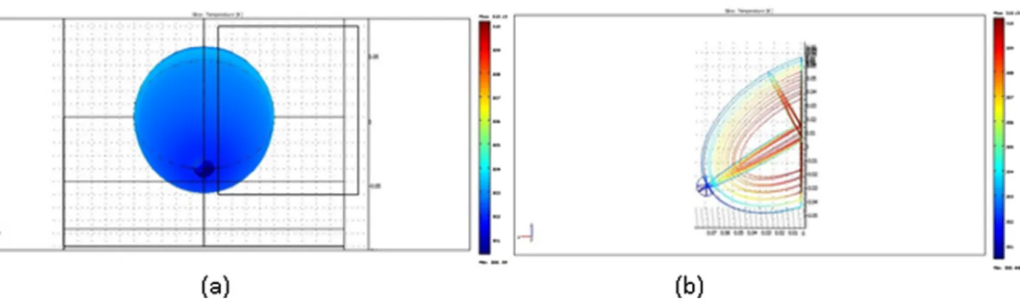
[6], it had four quadrants and four concentric tissue layers, representing the core glandular, subcutaneous glandular, fatty, and skin.Fig. 2a illustrates the desired shape schematically.
According to the average female breast geometry[11], the outer major and minor semi-axis lengths of the ellipsoid were set to 0.08 m and 0.05 m, respectively, and the distance between the layers was set on 0.005 m. Steady state solutions match experimental thermographic results by choosing the proper thermal properties [16]. Therefore, values of thermal conductivity (k), metabolic rates (qm), and blood perfusion terms (the product of specific heat capacity and blood mass flow rate) for various layers were taken from Werner and Buse
[17].
Sudharsan and Ng[18]reported that out of thousand cases screened, the percentage of women with carcinomas sizes of
11–15 mm, 16–20 mm, and 50 mm was respectively around 52%, 62%, and 95%. According to their findings, the average size of a tumour was 1.415 cm in spheroid shape when detected in clinics for the first time. Therefore, in the present study, the tumour was assumed to have a spherical shape and four tumour sizes with a range of 5 mm to 20 mm were considered. From Gautherie[11], the tumour metabolic heat generation rate and the doubling time are related as a hyperbolic function
qms¼cðW day=m
3Þ ð
10Þ whereqmis the tumour metabolic heat generation rate per unit volume (W/m3),sthe time required for the tumour to double its volume, also known as doubling time, andca constant and equal to 3.27106W day/m3. The relation between the tumour diameter, D, and the doubling time, s is shown in Eq.(11) [6,7,11].
D¼102exp 0½ :002134ðs50ÞðmÞ ð11Þ Since these simulations are performed for several tumour sizes, the correspondingqmfor each tumour size was calculated from Eq.(10)and(11). Thekandwbvalues of the cancerous tissue were taken to be 0.48 W/mC and 48 * 103W/m3 [11], respectively. In the present study, the off-axis tumour was con-sidered and the tumour depth was defined as the distance between the tumour surface and the breast surface.
The DTDs and STDs for tumours with four different diam-eters at a constant location are depicted inFig. 3a. Similarly,
Fig. 3b shows that temperature distributions of the tumour with 10 mm diameter in depth vary from 0.011 m to 0.035 m. As shown inFig. 3b, the increase in the tumour depth results in a significant decrease in the magnitude of the corresponding STD. Even if this minor temperature changes had been repre-sented by a pseudo-colour map, they could have hardly been detected by humans’ eyes[4].
The normal breast tissue was divided into sixteen layers with equal thickness, and then, the average temperature for each layer was calculated.Fig. 2b shows a cross-sectional view of the temperature distribution in each layer in a normal breast. The depth of the tissue layer versus the average temper-ature difference between the surface and depth in a normal breast model is illustrated inFig. 3c. The average temperature difference increases gradually from the surface to the chest wall base in a normal beast model.
As seen inFigs. 3a and 3b, by locating the tumour in each layer, the tumour induced contrast is added to the normal tem-perature of that layer. Therefore, to estimate tumour depth, the minimum (baseline) temperature in DTD is assumed to be the average temperature of the layer located at it. Finally, tumour depth was calculated usingFig. 3c.
Data preparation
Using the finite element analysis of the breast model, four tumour sizes (5 mm, 10 mm, 15 mm and 20 mm) at 10 different depths with 2 mm interval were simulated. For each tumour size and location, the depth temperature distribution (DTD) and the corresponding surface temperature distribution (STD) were extracted. These distributions were used for train-ing and testtrain-ing the dynamic neural network (overall 40 vectors, each vector has length around 70 samples). Since dynamic net-work is a sequential netnet-work, the samples of input–output data
pairs of static networks were replaced by input–output data sequences. These data sequences were divided into two subsets: 75% of the samples were assigned to the train set (30 vectors with around 2100 samples) and 25% to the test set (10 vectors with around 700 samples). Neural network training can be
made more efficient if certain pre-processing actions are per-formed on the network’s inputs and outputs. In this study, ini-tially, the linear trend was removed from the data in order to separate the tumour-induced thermal contrast from normal temperature distribution. This was carried out by computing Fig. 2 The rotated semi ellipsoid breast tissue model: (a) The normal surface temperature. (b) The temperatures of four concentric tissue layers with uniform thickness.
Fig. 3a The STDs and DTDs for different tumour sizes at constant depth: The red curves are STDs and the blue ones are DTDs.
Fig. 3b The STDs and DTDs for different tumour depths with constant size (Diam = 0.005 m): The red curves are STDs and the blue ones are DTDs.
the least-squares fit of a composite line to the data and sub-tracting the resulting function from the data.
Data adjustment
In order to apply the method to real data (thermal image), the model data had to be matched and normalized with thermal image data in both spatial and thermal scales. The minimum spatial distance between samples in thermal image is restricted by the camera field of view (FOV). In this study, the camera’s FOV (Thermoteknix Visir 640) was 19.5 * 25.8. In addition, participants were asked to stay 1 m away from the camera. Therefore, considering these parameters, vertical and horizon-tal dimensions of the image were calculated to be 0.4515 m and 0.34125 m, respectively. Considering resolution indexes (480 * 640) of the camera, the distance between samples in the image was 7.05 * 104m. This value was used as sampling interval in the model data. For this purpose, the interpolation function (interp1) of MATLAB software with cubic spline method was used.
For normalizing the thermal scale, the mapminmax func-tion of MATLAB software was applied to the image and model data. At the forward stage, the thermal range of all data was saved and data were mapped to the interval [1,+1] by applying the function to the model data. During the inverse stage, this function with saved conditions was reapplied to the image data so as to match it to the thermal scale.
Selection of optimal network structure
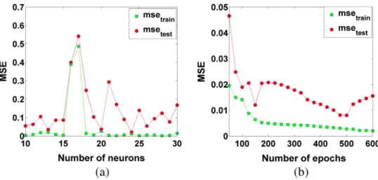
In order to avoid overtraining and obtain a system with acceptable performances, a number of neurons in the hidden layer and optimum number of epochs are crucial. Since deter-mining the dynamics and number of neurons and epochs are not independent on each other, so they are iteratively deter-mined. Initially, dynamics with forward selection method were selected by assuming a fixed number of neurons and epochs. Then, the optimum number of neurons with obtained dynam-ics and fixed epochs was determined. For this purpose, the number of neurons varied from 10 to 30 in 10 steps (Fig. 4a). Having trained the network with each number of neurons, the MSE of train and test data set was calculated.
Finally, the number of neurons in which the MSE of test data set had the minimum value was selected as an optimum num-ber of neurons. Similarly, with achieved dynamics and neu-rons, the optimum number of epochs was determined. For this purpose, the epoch number varied from 50 to 600 in 23 steps. InFig. 4b, the MSE of train and test data set was plotted versus epoch numbers. The procedure was iterated until these values remained fixed.
In the model, the simulator network has thirteen hidden layer neurons with Tanh activation functions and a single sat-urated linear function in the output layer. The Levenberg– Marquadt algorithm is applied to train the neural network. Five hundred (500) training iterations are performed, at the end of which the MSE is reduced to the order of 102. At this point, optimal network weights for the trained network are stored and used for validation. Training this neural network is a time consuming task. But it will not take too much time to test (the practical application) the trained network, an edge over iterative methods used in previous studies[8–10]. Valida-tion of the neural model on training data is shown inFig. 4c. As indicated inFig. 4c, the range of data presented to the neu-ral network indicates the entire range of data.
Neural network identification results in the forward step Once the neural network is trained with a suitable data set, it is ready to predict the DTD for a new data set not exposed to during the training phase. The network is validated for ten dif-ferent cases. As shown inFig. 4d, for each validation case, the output of the neural network model shows good agreement with simulation results with regard to R2 values (a measure of the goodness of fits). Simulation errors in the test data are shown in Fig. 4e. According to the results, the performance of the neural network is acceptable and simulation errors are not large.
Experimental data analysis
In order to apply the proposed method to the thermal image, thermography was conducted on twenty patients with histo-logically confirmed breast cancers with ages ranging from 22 to 55 years old (mean = 39 years, SD = 9 years) at the ‘‘Imam Fig. 3c Depth of tissue versus the average temperature difference between surface and depth.
Khomeini hospital” in Tehran, Iran.All procedures followed were in accordance with the ethical standards of the responsible committee on human experimentation (institutional and national) and with the Helsinki Declaration of 1975, as revised in 2008 (5). Informed consent was obtained from all patients for being included in the study.
The patients had tumour sizes ranging from 0.5 to 4 cm and tumour depths ranging from 1 to 3.5 cm. Infrared imaging was performed on all patients before they performed biopsy.
Breast thermal images were acquired by using the thermal camera (FLIR) with a spectral of 7–13lm. For this, partici-pants had to undergo 15 min of waist-up nude acclimation in a sitting position. A thermal image is captured from the frontal view of breasts and the corresponding temperature matrix is saved.
Temperature and humidity of the imaging room, with carpeted floor, must be controlled, free from heating sources. Relative humidity should fall between 4% and 75%[4]. The camera was fixed 90°to patients, and parallel to the ground when mounted on a parallax free stand[3,4].Fig. 5a shows the original thermal image.
There are four feature boundaries which enclose breasts, including left and right body boundaries and two lower bound-aries of breasts[19]. In order to extract these boundaries, the procedure explained in Saniei et al. [19] was applied. After
detecting target breast regions, corresponding temperature val-ues from temperature matrix were chosen as favourite temperatures.
Extraction of surface temperature distribution
To extract hot regions for detecting suspicious areas, different types of image segmentation methods can be applied. These methods are based on texture, colour, and intensity extracted from the thermal image[20,21]. Thermal image is expressed with pseudo-colour maps[22]. The graphical summary of tem-peratures is connected with little loss of information [4]. Accordingly, the present study used a processed temperature matrix for extracting hot regions.
In each breast’s temperature matrix, regions with degrees between maximum temperature and one degree lower the level were chosen as target areas. Since lower breast and armpit areas are intrinsically warmer than other parts, it is essential to eliminate them from suspicious areas. For this purpose, the extracted regions with distance less than 3 pixels from the breast boundaries were removed.
If the tumour shape is spherical, it will have a symmetrical bell-shape distribution at any position at the surface[23]and by choosing one line through the maximum temperature, this Fig. 4a and b (a) Effect of increasing the number of neurons on train and test error. (b) Effect of increasing the number of epochs on train and test error.
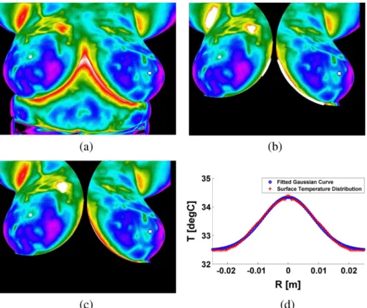
distribution can be achieved. But practically speaking, there are many lines (asymmetrical distribution in each direction) in tumour areas because of tumours’ asymmetrical shape. Therefore, just choosing one line for analysing is inappropri-ate. Since in the present study a two-dimensional area was analysed for extraction of STD, average distributions in differ-ent directions could be calculated. Therefore, the correspond-ing signal, which is a mean temperature distribution, reveals an uncertainty in estimating tumour’s parameters. Considering this, in the study, we used the approach proposed by Liu and colleagues for a better approximation of the distribution[24]. At first, coordinate of the maximum temperature was cho-sen as the centre to draw rectangles. Each rectangle has the same gap and every rectangle is divided by 30 lines, which is all through the rectangle centre. The number of rectangles is proportional to the maximum diameter of the suspicious region. Then every single line should be analysed to a value. The procedure continues with averaging whole 30 values to an average value. Finally, this value should be set as the rect-angle’s value. InFig. 5b–d the segmented hot region and its corresponding STD for a patient with right breast cancer are shown.
Finally for normalization of extracted STD as explained in Section ‘Numerical simulations of a breast model’, the
map-minmax function with saved conditions of model data was applied to map image data to interval [1,+1].
Experimental results and discussion
After the normalization process, the trained dynamic neural network was used to estimate DTD. Since DTD is the temper-ature distribution at the tumour surface and its surrounding tissue, in order to find tumour parameters the portion of tem-perature distribution, which matches with Eq. (5)the most, should be considered. Thus, by cutting data from the begin-ning and end in some steps and fitting Eq.(5)to it, the best function with minimum mse (mean square error) was chosen. Then, the coefficients of desired function were extracted to esti-mate the size and heat generation rate of tumours (Eq. (5)). Finally, by selecting the baseline temperature of DTD as the mean temperature layer and subtracting it from the mean tem-perature of the surface by using the graph introduced in
Fig. 3c, the depth was estimated.
Table 1 shows actual and estimated tumour sizes and depths for participants in the study. Also, the calculated meta-bolic heat generation rate is presented.Fig. 6a shows a com-parison of estimated and actual tumour diameters for all Fig. 4d Comparison of output of trained DNN with finite element simulation.
cases. Comparison of estimated and actual tumour depths is presented inFig. 6b. To estimate the model’s accuracy, a cor-relation coefficient (R2) was run. The corcor-relation coefficient,
which indicates how strong the linear relationship between two variables is, was found to be 0.84 and 0.71, respectively, for size and depth. Absolute errors in depth and size were Fig. 5 (a) The original image. (b) Segmentation of hot regions (the white regions). (c) Elimination of unwanted regions. (d) STD of the suspicious region.
Table 1 Results from parameter estimation procedure to determine embedded tumour parameters using surface temperature distribution.
Patient Age Pathological Pathological Estimated Estimated Heat generation rate (mW/cm3) # Tumour size (cm) Tumour depth (cm) Tumour size Tumour depth
1 42 1.1 2 0.95 1.89 68.642 2 29 3 1 2.7 1.02 26 3 33 2.4 2 1.98 1.7 40.973 4 38 1.2 2 1.5 2.47 56. 233 5 55 0.8 1 0.7 0.8 74.085 6 25 2 2.5 2.42 2.11 35.481 7 42 0.75 1 0.89 0.85 51.322 8 40 2.5 1.5 1.59 1.103 22.121 9 37 3.5 2 3.1 1.7 19.997 10 46 1.3 1 1.06 1.52 51.082 11 44 0.6 1.5 0.76 1.701 60.83 12 35 0.7 1.8 0.6 2 58.93 13 40 0.5 1 0.65 0.9 117.29 14 44 4 1.5 3.45 1.64 7.92 15 50 1.5 1 1.1 0.8 40.522 16 22 1.3 1.8 1.06 1.4 44.71 17 32 0.5 1.5 0.41 1.7 120.8 18 33 2.7 3.5 2 2.8 19.08 19 30 0.8 1.5 0.66 1.2 68.45 20 47 1.8 3 1.2 2.1 40.2
within 0.31 cm and 0.2 cm, respectively. Results showed that the depth estimation error was larger than the size estimation error. Also, deep seated tumours had higher error than other cases.
This less accurate estimation of tumour depth may be due to applying a simple breast model which did not account for gravity induced geometry, non-uniform layer thickness, differ-ent tumour shapes, and departure of individual thermal prop-erties from the population average used in this study. For increasing the accuracy of the suggested method, it is favour-able to analyse shape progress of tumours with stack-based layering theory[25]in future works.
Practical constraints of this method (accuracy and resolu-tion of thermograms) could be also other error sources. Because of restricted accuracy of thermal cameras or inade-quate knowledge about the emission coefficient, accuracy of temperature measurements is restricted. As reported in Ng’s study[4], the temperature of objects in a thermal image depen-dents on the angle of view because the emission coefficient of an object will change when infrared measurements are taken at various angles.
Findings of the study suggest that it is possible to determine required parameters from a pool of surface temperature data. In comparison with previous studies[8–10], the method
pro-posed in the study is more time effective. In general, findings were in agreement with actual parameters.
Conclusions
Thermography is a non-invasive, nonionizing, and efficient method for an early diagnosis of breast cancer. One basic ques-tion here is how complex relaques-tionships between breast thermal patterns and underlying heat source parameters can be quanti-fied. Using a thermography-based skin surface temperature profile, the present article introduced a simple methodology for estimation of breast tumour parameters. Data obtained from numerical simulations coupled with an approximate model and a dynamic neural network were used to address the inverse problem.
According to the analysis of the clinical cases with correla-tive theories, this method is practicable with certain usable val-ues. However, there have been several aspects which need to deal with, for example, the gravity induced geometry deforma-tion, non-uniform layer thickness and the departure of individ-ual thermal properties from the population average will have some impacts on the result of analyses. As a future work, the accuracy and reliability of the system can be improved by increasing the number of images.
Fig. 6a Comparison of actual tumour size with estimated tumour size.
The authors would like to thank Fanavaran Madoon Ghermez Co., for providing high-resolution thermal camera for taking the breast thermograms.
References
[1]Lawson RN. Implications of surface temperatures in the diagnosis of breast cancer. Can Med Assoc J 1956;75(4):309–10. [2]Gautherie M, Gros CM. Breast thermography and cancer risk
prediction. Cancer 1980;45(1):51–6.
[3]Etehadtavakol M, Ng EYK. Breast thermography as a potential non-contact method in the early detection of cancer: a review. Mech Med Biol J 2013;13(02):1330001.
[4]Ng EK. A review of thermography as promising non-invasive detection modality for breast tumor. Int J Therm Sci 2009;48 (5):849–59.
[5]Jiang L, Zhan W, Loew MH. Toward understanding the complex mechanisms behind breast thermography: an overview for comprehensive numerical study. In: SPIE medical imaging. International society for optics and photonics, 79650H-79650H.
[6]Ng EYK, Sudharsan NM. An improved three-dimensional direct numerical modelling and thermal analysis of a female breast with tumour. Proceedings of the institution of mechanical engineers, Part H: J eng in med 2001;215(1):25–37.
[7]Ng EY, Sudharsan NM. Computer simulation in conjunction with medical thermography as an adjunct tool for early detection of breast cancer. BMC Cancer 2004;4(1):17.
[8]Mital M, Pidaparti RM. Breast tumor simulation and parameters estimation using evolutionary algorithms. Model Simul Eng 2008 [Article N°4].
[9]Gonza´lez FJ. Non-invasive estimation of the metabolic heat production of breast tumors using digital infrared imaging. Quant InfraRed Thermogr J 2011;8(2):139–48.
[10]Jiang L, Zhan W, Loew MH. Modelling thermography of the tumorous human breast: From forward problem to inverse problem solving. Biomedical imaging: from nano to macro. IEEE international symposium on 2010:205–8.
overview for comprehensive numerical study. In: SPIE medical imaging. International Society for Optics and Photonics; 2011, 79650H-79650H.
[16]Ng EYK, Sudharsan NM. Effect of blood flow, tumour and cold stress in a female breast: a novel time-accurate computer simulation. Proceedings of the Institution of Mechanical Engineers. Part H: J Eng Med 2001;215(4):393–404.
[17]Werner J, Buse M. Temperature profiles with respect to inhomogeneity and geometry of the human body. J Appl Physiol 1988;65(3):1110–8.
[18]Sudharsan NM, Ng EYK. Parametric optimization for tumour identification: bioheat equation using ANOVA and the Taguchi method. Proceedings of the institution of mechanical engineers. Part H: J Eng Med 2000;214(5):505–12.
[19]Saniei E, Setayeshi S, Akbari M E, Navid M. A vascular network matching in dynamic thermography for breast cancer detection. Quant InfraRed Thermogr J 2015;12(1):24–36. [20]EtehadTavakol M, Sadri S, Ng EYK. Application of K-and
fuzzy c-means for color segmentation of thermal infrared breast images. J Med Syst 2010;34(1):35–42.
[21]Golestani N, EtehadTavakol M, Ng EYK. Level set method for segmentation of infrared breast thermograms. EXCLI J 2014;13:241–51.
[22]EtehadTavakol M, Ng EYK, Lucas C, Sadri S, Gheissari N. Estimating the mutual information between bilateral breast in thermograms using nonparametric windows. J Med Syst 2011;35 (5):959–67.
[23]Sudharsan NM, Ng EYK. The surface temperature distribution of a breast with and without tumour. Computer Methods Biomech Biomed Eng 1999;2(3):187–99.
[24]Liu Y, Li KY, Zhang XL, Sun SR, Wan YW. Analyzing method of the inner heat source in breast based on infrared imaging and clinical application. In: 1st international conference on bioinformatics and biomedical engineering. p. 853–6.
[25]Dorrah HT. Consolidity: stack-based systems change pathway theory elaborated. Ain Shams Eng J 2014;5(2):449–73.