Unsupervised and supervised data classification via
nonsmooth and global optimization
1A. M. Bagirov, A. M. Rubinov, N.V. Soukhoroukova and J. Yearwood
School of Information Technology and Mathematical Sciences, The University of Ballarat, Vic 3353, Australia.
Abstract
We examine various methods for data clustering and data classification that are based on the minimization of the so-called cluster function and its modifications. These functions are nonsmooth and nonconvex. We use Discrete Gradient methods for their local mini-mization. We consider also a combination of this method with the cutting angle method for global minimization. We present and discuss results of numerical experiments.
Key words: clustering, classification, cluster function, nonsmooth optimization, global op-timization
1
Introduction
With the rapid increase in the availability of data for exploration and analysis it is important to develop techniques that efficiently perform data clustering and data classification. In the first case there is a need to get insight into the data and find out things about it in as objective a way as possible. This type of approach is usually classed as exploratory data analysis and includes clustering. The second concerns learning or identifying the extent to which the data conforms to known or hypothesized models.
Clustering or cluster analysis involves the identification of subsets of the data that are similar. The subset usually intuitively corresponds to points that are more similar to each other than they are to points from another cluster. Points in the same cluster have the same label. Clustering is carried out in an unsupervisedway by trying to find subsets of points that are similar without having a predefined notion of the cluster. We can say that the identification of these clusters with labels is data driven rather than determined by a particular model or view of the data.
Classification involves the supervised assignment of data points to predefined and known classes. Here, there is a collection of classes with labels and the problem is to label a new observation or data point as belonging to one or more of the classes. Usually the known classes of examples constitute atraining setand are used to learn a description of the classes. This can then be used to assign new examples to classes. The classes are determined by some a priori knowledge about the dataset.
1
1.1 Clustering
According to Jain [51], the clustering task usually involves the following steps: 1. representation of the data;
2. deciding on a similarity measure or distance metric that is most appropriate for the task in the domain;
3. performing the clustering; 4. cluster description; 5. evaluation.
Data representation is the task of deciding the number of features available, their nature and scale, the size of the dataset and the number of clusters or classes. Feature selection is the process of selecting a set of features that are the most effective subset to use with the clustering algorithm. Feature selection methods are used to identify the most informative features, to remove some uninformative or noisy features and reduce the dimension of the problem under consideration. Feature extraction or feature combination is the use of transformations of the feature set to produce a set of features that are able to be effectively used by the clustering algorithm.
In many problems of cluster analysis, there is little prior information available about the data, and as few assumptions about the data as possible can be made. It is under these restrictions that clustering methodology appropriate for the exploration of interrelationships among data points can be used to make assessments of their structures.
The notion of clustering is relatively flexible as the aim is to identify and reveal clusters or groups in an exploratory data analysis sense. An important concept is that of a cluster representative also called cluster profile, classification vector, cluster label, or centroid. It is simply an object that summarises and represents the objects in the cluster. It should be close to every object in the cluster in some average sense. The similarity of the objects to the objects is measured by a matching function or similarity function.
The notion of similarity is crucial in the definition of clustering. Similarityis usually measured by some dissimilarity measure such as a metric defined on the dataset. However there are other ways of approaching the definition of similarity. For example, Finnie and Sun [41] define a similarity relation as an equivalence relation. This would then imply that similarity is a transitive notion which is stronger than what we usually expect in the notion of similarity. Most clustering algorithms use a number of empirically determined parameters such as:
• the number of clusters
• a minimum and maximum size of each cluster
• a threshold value on the matching function, below which an object will not be included in a cluster
• a control on overlap between clusters
1.2 Clustering Techniques
In clustering, data or observations are usually represented asfeature vectorsand the individual scalar components of a feature vector x = (x1, . . . xn) are called features or attributes. The dimensionality of the data or the dataset is n.
In selecting or developing clustering techniques the method should exhibit some theoretical soundness. This may be assessed by certain criteria of adequacy. Some criteria that have been suggested by Jardine and Sibson [52] are:
1. the method produces a clustering which is unlikely to be altered drastically when addi-tional objects are incorporated - stability under growth;
2. the method is stable in the sense that small perturbations in the description of the objects lead to small changes in the clustering;
3. the method is independent of the initial ordering of the objects. 1.2.1 Hierarchical Clustering
A hierarchical algorithm produces a dendrogram presenting a nested grouping of data and similarity levels at which the clusters change. Most hierarchical clustering algorithms are variants of the single link [85], the complete link [56] and minimum variance [88, 71] algorithms. The single-link approach takes as the distance between two clusters, the minimum of the distances between all pairs of points in the two clusters (one from the first cluster, the other from the second). The complete-link algorithm takes the distance between clusters as the
maximum of all pairwise distances between points in the two clusters. The complete-link algorithm produces compact clusters [8] whereas the single link algorithm tends to produce clusters that are elongated due to a chaining effect [72].
1.2.2 Partitional Algorithms
A partitional clustering algorithm produces a single partition of the data with no hierarchical structure. This means that the algorithm usually requires the number of clusters to be speci-fied. They usually optimize a criterion function defined on the dataset. Most algorithms have traditionally been run multiple times with different starting states and the best configuration produced is the one used as the clustering. The most frequently used objective function is the squared error criterion
fk(x) = k X j=1 nj X i=1 ka(ij)−xjk2,
where k is the number of clusters, nj is the number of records in the cluster j, j = 1, . . . , k, a(ij) is the i-th element of the clusterj,i= 1, . . . , nj and xj is the centroid of thejth cluster: xj = (1/nj)Pni=1j a
(j)
i . This has been found to work well with isolated and compact clusters. The k-means algorithm is the most commonly used algorithm using this criterion [66] The k-means algorithm randomly chooses k cluster centres and iteratively reassigns data points to clusters based on the similarity between the pattern and the cluster centers until
there is no further reassignment or the squared error no longer decreases significantly. It is popular because it is easy to implement with time complexity O(n). It suffers from being sensitive to the selection of the initial clustering partition or cluster centres. Several variants of the k-means algorithm have been reported in the literature [3], many of them focussing on the selection of a good initial partition.
1.2.3 k-Nearest Neighbour Clustering
In this approach, each unlabelled data point is assigned to the cluster of its knearest labelled neighbours as long as the average distance to the kneighbours is below a threshold [60]. 1.2.4 Connectionist techniques
Artificial neural networks (ANNs) have been used extensively for both classification and clus-tering [83]. The most common ANNs used for clusclus-tering include Kohonen’s learning vector quantization (LVQ) and self organizing map (SOM) [58] and adaptive resonance theory (ART) models [33]. These networks have simple architectures with single layers and the weights are learnt by iteratively changing them until a termination criterion is satisfied. These learning or weight changing procedures are similar to some used in classical clustering approaches. For example the procedure used in the LVQ is similar to the k-means algorithm.
The SOM is often used because it generates an intuitive two dimensional map of a multidimen-sional dataset but it generates a suboptimal partition if the initial weights are not properly selected.
There are two major concerns for ANN learning:
• stability - no point in the training set changes its class after a finite number of learning steps
• plasticity - the ability of the algorithm to adapt to new data
For stability the learning rate should decrease to zero as iterations proceed but this affects the plasticity.
Shang and Wah [84] describe a global optimization approach for the determination of network weights with layered feed-forward networks and attribute the finding of better local minima to the global search stage.
1.2.5 Mixture Models
In the mixture model approach to cluster analysis the underlying assumption is that the data are drawn from a mixture of an initially specified number k of groups in some proportions
π1, . . . , πk. That is, the data come from a population whose distribution is the mixture probability density function
f(y; Ψ) = k
X
i=1
where the k components correspond to thekgroups. Here the vector Ψ of unknown parameters consists of the mixing proportions πi and the elements of theθi knowna priorito be distinct. On specifying a parametric form for each component p.d.f ci(y;θi), Ψ can be estimated
by maximum likelihood or some other method. Once the mixture model has been fitted, a probabilistic clustering of the data into k clusters can be obtained in terms of the fitted posterior probabilities of component membership for the data. An outright assignment of the data into the k clusters is achieved by assigning each data point to the component to which it has the highest estimated posterior probability of belonging.
Most of the work in this area has assumed that the individual components of the mixture density are Gaussian and in this case the parameters of the individual Gaussians are to be estimated. More recently, the Expectation Maximization (EM) algorithm has been applied to this problem of parameter estimation [65].
1.2.6 Evolutionary Approaches
One of the most well known heuristic approaches to global optimization is the genetic al-gorithm. Genetic algorithms (GAs) [49, 44] are an example of a set of approaches known as evolutionary approaches motivated by the ideas of natural selection and evolution. These approaches use evolutionary operators such asselection, recombinationandmutationon a pop-ulation usually encoded as chromosomesto obtain a globally optimal partition of the dataset. In GAs the selection operator propagates solutions from one generation to the next based on their fitness. Selection operators usually use a probabilistic scheme where chromosomes with higher fitness have a higher probability of being reproduced in the next generation.
Points in the search space (chromosomes) are represented as bit strings. The crossover oper-ator as a form of recombination exchanges subsequences of these bit strings between parents and is effective at exploring the search space and mutation acts as a fine tuning for the explo-ration process. GAs and other evolutionary strategies have been used to solve the clustering problem by viewing it as a minimization of the squared error criterion. Theoretical issues of convergence of these approaches are discussed in Fogel [42].
Whereas most traditional clustering techniques (such as k means, c-means and ANNs ) per-form a local search to optimize the objective function GAs perper-form a global search. One of the main problems in the use of GAs in clustering is the representation of the problem using bit strings. There have been many approaches (see Raghavan and Birchand [74], Bhuyan et al. [32] and Jones and Beltramo [55]) to the representation and crossover problems but most restrict the use of GAs on practical datasets to a small number of clusters. Representations which are of low order and short in defining length are required. Babu and Murty [7] im-plement a hybrid approach where the GA is used to find good initial cluster centres and the
k-means algorithm is used to find the final partition.
Another problem with GAs is their sensitivity to the selection of various parameters such as the population size and the mutation and crossover probabilities. This problem has been studied (for example see Grefenstette [45]) but there are still difficulties in achieving good results on specific problems. There have been claims that hybrid genetic algorithms incorporating problem specific heuristics are effective for clustering [55].
In many cases GA approaches perform better thank-means orc-means. However, all of these approaches suffer from sensitivity to the selection of the control parameters. For each specific
problem, there needs to be fine tuning of the parameter values to suit the application. 1.2.7 Fuzzy Clustering
Traditional or hard clustering approaches generate partitions or groups where each data point belongs to one and only one cluster. Fuzzy clustering extends the idea into the multi-label
domain where data points may be simultaneously in many clusters. Fuzzy clustering extends this notion to associate each data point with with every cluster using a membership function. The output of these algorithms is therefore a clustering rather than a partition. A fuzzy algorithm would usually select an initial fuzzy partition of thendata points intokclusters by initialising then×kmembership matrixU. Compute the value of a fuzzy objective function such as f(U) = n X i=1 k X j=1 uijkxi−cjk2
where cj =Pni=1uijxi is thejth fuzzy cluster centre and reassign data points to clusters to
reduce this objective function.
In a fuzzy clustering of data, larger values of the membership function for particular clusters indicate higher confidence in the assignment of that data point to that cluster. A hard clus-tering can be obtained from a fuzzy clusclus-tering by deciding on threshold values for membership values. A common fuzzy clustering algorithm is the fuzzy c-means (FCM) algorithm. It is usually better at avoiding local minima, than the k-means algorithm but can still converge to local minima of the squared error criterion. The design of the membership functions is an important problem in fuzzy clustering.
1.2.8 A simulated Annealing Approach
The simulated annealing approach is a sequential stochastic search technique modelled on the annealing of crystals. Simulated annealing algorithms are designed to avoid and recover from solutions which are local minima of the objective function. The technique achieves this by accepting with some probability a new solution of lower quality for the next iteration. The probability of acceptance is governed by a parameter called the temperature which is varies from a starting value at the first iteration to a final value at the final iteration. A simulated annealing clustering algorithm randomly selects an initial partition of the dataset, values for the initial and final temperatures and computes the squared error. Points are reassigned to clusters on the basis of the square error value either with a temperature dependent probability or not. At each iteration the value of the temperature is reduced.
Simulated annealing can be slow to reach an optimal solution. Optimal solutions require the temperature to be decreased very slowly over iterations. Selim and Al-Sultan [82] have studied the effects of the control parameters. Simulated annealing is statistically guaranteed to find the global optimal solution [2].
1.3 Data Classification
Classification is the supervised assignment of data points to predefined and known classes. Here, there is a collection of classes with labels and the problem is to label a new observation
or data point as belonging to one or more of the classes. The objective in many cases (where the data can be represented as real valued) is to learn a function f : Rn → yi :i= 1. . . n from the training data. Here the known classes of examples in the training set are represented by the labels yi. This function can then be used to assign new examples to classes. The problem is to estimate f so that the predicted label f(x) is the true label y for examples
x, y) which were generated from the same underlying probability distribution. The problem as represented above determines a classification function or classifier f that predicts many classes but only assigns a single class to each data point. There are classification problems that require a fuzzy prediction and these are usually termed multi-label classification problems. Furthermore classifiers are usually binary but the more general multi-class problem can be solved by the learning of several binary classifiers.
Convex programming technique also can be applied for data classification. We consider here only support vector machine technique.
The field of data classification is very large and covers a broad range of areas including biology, information science and bio-informatics. A good review of machine learning, neural and statistical approaches including decision tree algorithms such as C4.5 can be found in Michie et al [67].
1.3.1 Support Vector Machines
From statistical learning theory it is crucial that the class of classifier functions must be restricted to one with an appropriate capacity for the available training data. One such measure of capacity is theVC dimension- a measure of the function complexity. For a classifier to generalize from the training data to unseen examples it should be from a class of functions whose capacity can be computed and the algorithm should keep the capacity low as well as fit the training data.
Support vector machine classifiers are based on the class of hyperplanes
hw, xi+b= 0
w, x∈Rn, b∈IR corresponding to binary decision functions
f(x) = sign (hw, xi+b).
It is possible to prove that the optimal hyperplane, defined as the one with the maximal margin of separation between the two classes comes from the function class with the lowest capacity. This hyperplane can be constructed by solving a constrained quadratic optimization problem whose solution has w has an expansion in terms of a subset of the training data that that lie closest to the boundary. These training points, called support vectors, carry all relevant information about the classification problem. It is simple to show that the margin is inversely proportional to kwk and that the problem is:
minimize(hw, wi) subject to yi[hw, xii+b]≥1. The final decision function can be written as
where the index i covers only the support vectors. That is, if all data points other than the support vectors were removed, the algorithm would find the same solution. This property of
sparseness is important in the implementation and analysis of the algorithm. The quadratic programming problem and the final decision function depend only on inner products between data and this permits the generalization of this approach to the nonlinear case via kernel functions.
The main idea underlying kernel methods is the embedding of the data into a higher dimen-sional vector space. This allows the use of linear algebra techniques and geometry to detect structure in the data [80].
SVMs have achieved impressive results in classification tasks including text categorization [54], handwriting digit recognition [36] and with gene expression data for gene function prediction [31]. They have out performed most other approaches in most problem areas.
2
Cluster analysis via nonsmooth optimization
2.1 Introduction
Clustering is theunsupervised classification of patterns.
In cluster analysis we assume that we have been given a set A of a finite number of points of
n-dimensional space IRn, that is
A={a1, . . . , am}, whereai ∈IRn, i= 1, . . . , m.
There are different types of clustering such as partitional, packing, covering and hierarchical clustering. In this paper we will consider partitional clustering.
The subject of cluster analysis is the partition of the setAinto a given numberkof overlapping or disjoint subsetsAi, i= 1, . . . , k with respect to predefined criteria such that
A= k
[
i=1
Ai.
The sets Ai, i= 1, . . . , k are called clusters.
There exist different approaches to clustering including agglomerative and divisive hierarchical clustering algorithms as well as algorithms based on mathematical programming techniques. Descriptions of many of these algorithms can be found, for example, in [40, 50, 86]. An excellent up-to-date survey of existing approaches is provided in [51] and a comprehensive list of literature on clustering algorithms is available in this paper.
The clustering problem is said to behard clusteringif every data point belongs to one and only one cluster. Unlike hard clustering, the clusters are allowed to overlap in the fuzzy clustering
approach. In this paper we generally consider the hard unconstrained clustering problem, that is, we additionally assume that
Ai\Aj =∅, ∀i, j= 1, . . . , k, i6=j.
and no constraints are imposed on the clusters Ai, i = 1, . . . , k. Thus every point a ∈A is contained in exactly one and only one set Ai.
Many authors reduced the clustering problem to the following optimization problem (see, for example, [25, 26, 86]): minimize ϕ(C, x) := 1 m k X i=1 X a∈Ai kxi−ak22 (2.1) subject to C ∈ C, x= (x1, . . . , xk)∈IRn×k, (2.2) where kxk2 is the Euclidean norm, C = {A1, . . . , Ak} is a set of clusters, C is a set of all possiblek-partitions of the setAandxi is the center of the clusterAi, i= 1, . . . , k. (We shall discuss the notion of the system of centres of clusters later on.) The following problem also can be considered instead of (2.1)–(2.2):
minimize ϕ1(C, x) := 1 m k X i=1 X a∈Ai kxi−ak (2.3) subject to C ∈ C, x= (x1, . . . , xk)∈IRn×k. (2.4) The problem (2.3)–(2.4) depends on the choice of a norm: different norms can lead to dif-ferent centers of clusters. Since clustering is a ”flexible” notion, the use of difdif-ferent norms is acceptable.
The following form of (2.1)–(2.2) is more suitable for the application of optimization tech-niques: minimize g(x, w) := 1 m m X i=1 k X j=1 wijkxj−aik2 (2.5) subject to x= (x1, . . . , xk), xj ∈IRn, j = 1, . . . , k, (2.6) and k X j=1 wij = 1, i= 1, . . . , m, wij = 0 or 1, i= 1, . . . , m, j = 1, . . . , k, (2.7)
where k is the number of clusters (given), m is the number of available patterns (given),
xj ∈IRn is the j-th cluster’s center (to be found),wij is the association weight of patternai with cluster j (to be found), given by
wij =
1 if pattern iis allocated to cluster j ∀i= 1, . . . , m, j= 1, . . . , k, 0 otherwise.
Here wis anm×kmatrix. This is a mixed problem (it contains both continuous and integer variables).
The objective function g(x, w) of (2.5) has many local minima. Different methods of mathe-matical programming can be applied to solve this problem. Some review of these algorithms can be found in [47] with dynamic programming, branch and bound, cutting planes and the
k-means algorithms being among them. The dynamic programming approach can be effec-tively applied to the clustering problem when the number of instances m≤20,which means that this method is not effective for solving real-world problems (see [53]). Branch and bound algorithms are effective when the database contain only hundreds of records and the number of clusters is not large (less than 5) (see [39, 46, 47, 59]). For these methods the solution
of large clustering problems is out of reach. This leads to the usage of local techniques and different heuristics for solving large clustering problems. One of the popular techniques is the well-known k-means algorithm, which serves for the search of local minima of a problem that is equivalent to (2.1)–(2.2).
Much better results have been obtained with metaheuristics for global optimization, such as simulated annealing, Tabu search and genetic algorithms [75]. The simulated annealing approaches to clustering have been studied, for example, in [30, 82, 87]. Application of tabu search methods for solving clustering is studied in [1]. Genetic algorithms for clustering have been described in [75]. The results of numerical experiments, presented in paper [5] show that even for small problems of cluster analysis when the number of entities m≤100 and the number of clusters k≤5 these algorithms take 500-700 (sometimes several thousands) times more CPU time than the k-means algorithms. For relatively large databases one can expect that this difference will increase. This makes metaheuristic algorithms of global optimization ineffective for solving many clustering problems.
An approach to clustering analysis based on bilinear programming techniques has been de-scribed by Mangasarian in [63]. If a polyhedral distance, such as the 1-norm distance, is used, the cluster analysis problem can be formulated as that of minimizing the product of two linear functions on a set determined by satisfying a system of linear inequalities. The
k-median algorithm consisting of solving a few linear programs leads to a stationary point. The paper [16] describes a global optimization approach to clustering and demonstrates how the supervised data classification problem can be solved via clustering. A detailed presenta-tion of the main ideas from [16] can be found in [18]. The objective funcpresenta-tion in the problem from [18] is both nonsmooth and nonconvex and this function has a large number of local minimizers. Problems of this type are quite challenging for general-purpose global optimiza-tion techniques. Due to the large number of variables and the complexity of the objective function, general-purpose global optimization techniques as a rule fail to solve such problems. Objective functions of optimization problems that are equivalent to (2.1)–(2.2) usually have very many shallow local minima, which do not provide a good description of the dataset. However, as mentioned above, global optimization techniques are highly time-consuming. It is very important, therefore, to develop clustering algorithms based on optimization techniques that compute “deep” local minimizers. Such minimizers provide a good enough description of the dataset under consideration. Indeed, since clustering is a flexible notion, a deep local minimizer may satisfactory describe the clustering structure of this dataset. A different ap-proach, which can be successfully used for supervised classification, is to change the setting of the optimization problem under consideration and consider a series of simpler problems (step-by-step approach). Some versions of this step-by-step approach can also be used for clustering.
Datasets under consideration usually contains two types of features (coordinate of a vector): continuous and categorical. Continuous features usually reflect results of some measurements. A feature is called categorical, if it is either nominal or ordinal. A variable is a “nominal” one if its values only numerical codes of possible different states of the corresponding feature. If the states of a nominal variable can be arranged in a meaningful order, the term “ordinal variable” is used.
Our experience demonstrates that optimization algorithms work much better when a dataset contains only vectors with continuous features. However optimization algorithms can also be
used for some datasets with categorical features (see, for example, Subsection 3.10).
2.2 The nonsmooth optimization approach to clustering
Here we describe an approach to clustering from [18]. This approach leads to a nonsmooth and non-convex optimization problem, which is equivalent to (2.3)– (2.4), but simpler from the computational point of view.
We consider ann-dimensional space IRnequipped with a normk · k. As a rule we assume that
k · k=k · kp, p≥1, where kxkp = n X l=1 |xl|p !1/p , 1≤p <+∞.
The l-th coordinate of a vector x∈IRn is denoted byxl.
Consider a set A of m n-dimensional vectors a = (a1, . . . , an). The aim of clustering is to represent this set as the union of k clusters. We accept the hypothesis that each cluster can be described by a point that can be considered as its center. So we need to locate a cluster’s center in order to adequately describe the cluster itself. Thus, we would like to find kpoints that serve as centers of k clusters A1, . . . , Ak. First we need to give the formal definition of the centres of a finite system of finite mutually disjoint sets A1, . . . , Ak, having in mind that these sets are unknown and we know only their union.
Consider an arbitrary set X, consisting of k points x1, . . . , xk. The distance d(a, X) from a point a∈A to this set is defined by
d(a, X) = min s=1,...,kkx
s−ak.
The deviation d(A, X) from the setA to the setX can be calculated as
d(A, X) = X a∈A d(a, X) = X a∈A min s=1,...,kkx s−ak.
We say that the set ¯X= (¯x1, . . . ,x¯k) is the set of centres ofkclusters of the setAifd(A,X¯)≤
d(A, X) for each X = (x1, . . . , xk). Thus the search for centres of clusters (hence, the search for the clusters) can be reduced to the following unconstrained minimization problem:
minimize Ck(x1, . . . , xk) subject to (x1, . . . , xk)∈IRn×k, (2.8) where Ck(x1, . . . , xk) = 1 m X a∈A min s=1,...,kkx s−ak. (2.9)
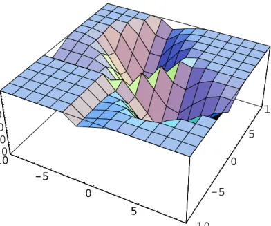
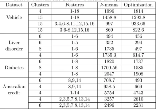
The functionCk defined by (2.9) will be called thecluster function. Figure 1 illustrates a plot of the cluster function C2 in IR1 for a dataset with 20 points.
Ifk >1, the cluster function is nonconvex and nonsmooth. It can be shown that this function has very many shallow local minimizers, which are close each to other.
Note that the number of variables in the optimization problem (2.8) isk×n. If the numberk
-10 -5 0 5 10-10 -5 0 5 10 0 10 20 30 40 50 -10 -5 0 5 10
Figure 1: Cluster function in IR2
problem. Moreover, the form of the objective function in this problem is complex enough not to be amenable to the direct application of general-purpose global optimization methods. Therefore, in order to ensure the practicality of the nonsmooth optimization approach to clustering, proper identification and use of local optimization methods is very important. Clearly, such an approach does not guarantee a globally optimal solution to problem (2.8). However, because clustering is a flexible notion, we do not need to obtain the exact solution of (2.8), it is enough to have a good approximation of this solution. This approximation can be accomplished by a “deep” enough local minimum of the cluster function. We can suppose that a deep local minimizer provides a good enough clustering description of the dataset under consideration. Thus we will be concerned with the search for “deep” local minima. The local method for non-smooth optimization that we use (see Section 4) can avoid saddle points and even some shallow local minimizers. Combination of this method with some global techniques can help to attain a deep local minimizer.
The following version of the problem (2.8) can be considered: minimize 1 m X a∈A min s=1,...,kkx s−ak2 subject to (x1, . . . , xk)∈IRn×k, (2.10) where k · kis 2-norm.
It is shown in [25] that problems (2.1)–(2.2), (2.5–2.7) and (2.10) are equivalent. The number of variables in problem (2.5)–(2.7) is (m+n)×k whereas in problem (2.10) this number is only n×kand the number of variables does not depend on the number of instances. It should be noted that in many real-world databases the number of instancesmis substantially greater than the number of features n. On the other hand the coefficients wij are integer in hard clustering problems, that is the problem (2.5)–(2.7) contains both integer and continuous variables. We have only continuous variables in the nonsmooth optimization formulation
of the clustering problem. All these circumstances can be considered as advantages of the nonsmooth optimization formulation (2.8) and its version (2.10).
2.3 Cluster function as a tool for measuring the fitness of a collection of points
Very often we have different candidate vectors X = (x1, . . . , xk) which contend to be con-sidered as centres of clusters. It is an important task to compare these candidates. We now describe the simplest situation where we need such a comparison. Assume that we use a cer-tain local method for the search for centers of clusters. We can run this method many times from different initial points. As a rule we obtain different results. How is the best among them chosen?
We can use the cluster function for the comparison. Assume that a norm k · k is fixed and we consider the cluster function f generated by this norm. It follows directly from the definition of the cluster function, that the candidateX∗= (x1∗, . . . , xk∗) is better suited for the role of centres of clusters than candidate X = (x1, . . . , xk) in the sense of the norm k · k if
Ck(x1∗, . . . , xk∗)< Ck(x1, . . . , xk).
2.4 k-means algorithm
The k-means algorithm is one of the effective algorithms for solving clustering problems on large datasets. Different versions of this algorithm have been studied by many authors (see [86]). This algorithm is based on the the minimization of the variation within clusters and the maximization of the variation between clusters. The variation depends on the chosen norm. Usually the norm k · k2 is used for this purpose, however versions of k-means with different norms also can be used. For simplicity we describe the simplest version of this method (see, for example, [69]) which was developed by MacQueen in 1967 (see [61]). In this paper we use this version and also its modification, wherek · k1 is used instead of k · k2.
The method starts with a user-specified value of k (number of clusters) points. To sort m
observations into k clusters with a given normk · k , we use the following procedure. 1. Take any kobservations as the centers of the first kclusters.
2. Assign the remaining m−k observations to one of the k clusters on the basis of the shortest distance (in the sense of the norm we choose) between the observation and the center of the cluster.
3. After each observation has been assigned to one of thekclusters, the centers are recom-puted (updated) as the centroids of found clusters.
Stopping criteria: there is (almost) no observation, which moves from one cluster to another.
k-means is a very fast algorithm and it is suitable for solving clustering problems in large databases. This algorithm gives good results when there are only a few clusters but dete-riorates when there are many [47]. If k · k2 is used then k-means achieves a local minimum of problem (2.1)( see [81]), however experiments show that the best clustering found with
k-means may be more than 50 % worse than the best known one [47]. This is because, the
k-means, like the majority of local methods, is very sensitive to the choice of the initial point. These experiments shows that k-means usually leads to a shallow local minimum of (2.1), which does not describe the cluster structure well.
2.5 An optimization clustering algorithm
A meaningful choice of the number of clusters is very important for clustering analysis. It is difficult to definea priorihow many clusters represent the setAunder consideration. In order to increase the knowledge generating capacity of the resulting clusters, the decision maker has to start from a small enough number of clusters k and to gradually increase the number of clusters for the analysis until certain termination criteria motivated by the underlying decision making situation as satisfied. From an optimization perspective this means that if the solution of the corresponding optimization problem (2.8) is not satisfactory, the decision maker needs to consider problem (2.8) with k+ 1 clusters and so on. This implies that one needs to solve repeatedly arising global optimization problems (2.8) with different values of k - a task even more challenging than solving a single global optimization problem. In order to avoid this difficulty, we suggest a step-by-step calculation of clusters.
The main idea of the proposed algorithm (see [22]) is to use the results obtained at a certain step for finding a good initial state for the next step. Note the cluster function for k = 1 is convex, so we can use convex programming techniques if k= 1.
The proposed approach has two distinct important and useful features:
• it allows the decision maker to successfully tackle the complexity of large datasets as it aims to reduce the number of data instances (records) of the dataset under consideration without loss of valuable information
• it provides the capability of calculating clusters step-by-step, gradually increasing the number of data clusters until termination conditions are met, that is it allows one to calculate as many cluster as a dataset contains with respect to some tolerance.
Algorithm 2.1 An algorithm for solving a cluster analysis problem.
Step 1. (Initialization). Select a tolerance ε > 0 and an positive integer k0 as the starting number of clusters. Select a starting point x0 = (x01, . . . , x0n, . . . , xk0
1 , . . . , xkn0) ∈ IRn×k0 and solve the minimization problem (2.8) with k = k0. Let x1∗ ∈ IRn×k0 be a solution to this problem and C1∗ be the corresponding objective function value. Setk=k0.
Step 2. (Computation of the next cluster center). Select a point x0 ∈ IRn and solve the following minimization problem of the dimension n:
minimize C¯k(x) subject to x∈IRn (2.11) where ¯ Ck(x) = X a∈A minnkx1∗−ak, . . . ,kxk∗−ak,kx−ako.
Step 3. (Refinement of all cluster centers). Let ¯xk+1,∗ be a solution to problem (2.11). Take
xk+1,0 = (x1∗, . . . , xk∗,x¯k+1,∗) as a new starting point and solve (2.8) with the objective function Ck+1.
Step 4. (Stopping criterion). Let xk+1,∗ be a solution to the problem (3.4) andCk+1,∗ be the corresponding value of the objective function. If
Ck∗−Ck+1,∗
C1∗
< ε
then stop, otherwise set k=k+ 1 and go to Step 2.
In Step 1 the centers of the firstk0 clusters are calculated. In particular, one can takek0 = 1, then the center of the entire set A will be calculated. In Step 2 we calculate a center of next (k+ 1)-st cluster, assuming previous k cluster centers to be known. Note that the number of variables in problem (2.11) is n which is substantially less the number of variables when all cluster centers are calculated simultaneously. In Step 3 the refinement of all k+ 1 cluster centers is carried out. It is quite possible that the starting point xk+1,0 calculated in the previous Step 2 is not far from the solution to problem (2.8), so it takes only a moderate number of iterations to calculate this solution. Such an approach allows significant reduction in the computational time for solving problem (2.8).
It is clear that Ck∗ ≥0 for allk≥1 and the sequence {Ck∗} is decreasing:
Ck+1,∗ ≤Ck,∗ for all k≥1.
Hence after ¯k >0 iterations the stopping criterion in Step 4 will be satisfied.
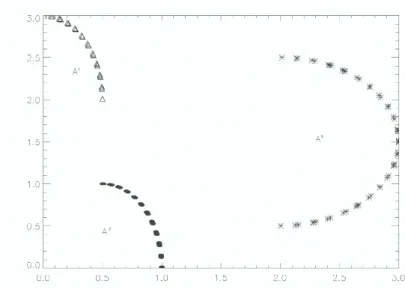
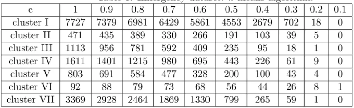
One of the important questions when one tries to apply Algorithm 2.1 is the choice of the tolerance ε >0. Large values of εcan result the appearance of large clusters whereas small values can produce small and artificial clusters. In order to explain this, let us consider an artificial dataset on IR2 as shown in Figure 2. There are three isolated clusters in this dataset given by the following formulae, respectively:
A1 = ak ∈IR2 :ak= (ak1, ak2), ak1 = 1 2|sin(k)|, a k 2 = 2 +|cos(k)|, k = 1, . . . ,50 , A2 = ak∈IR2 :ak= (ak1, ak2), ak1 = 1 2(1 +|sin(k)|), a k 2 =|cos(k)|, k = 1, . . . ,50 , A3 =nak∈IR2 :ak= (ak1, ak2), ak1 = 2 +|cos(k)|, ak2 = 1.5 + sin(k), k= 1, . . . ,50o.
If ε = 10−1 then Algorithm 2.1 exactly calculates these three clusters, if ε= 10−2 then this algorithm divides the third cluster into three clusters. When ε is smaller we have further division of these clusters. So if ε is small enough we obtain some artificial clusters. The results of numerical experiments show that the best values for εareε∈[10−1,10−2].
Figure 2: Three clusters in IR2
2.6 Results and discussion
To verify the effectiveness of the clustering algorithm a number of numerical experiments with middle-sized and large datasets have been carried out on a Pentium-4, 1.7 GHz, PC.
First we consider three standard test problems to compare our algorithm with k-means and metaheuristics: the tabu search (TS) method, a genetic algorithm (GA) and a simulated annealing (SA) method. We use the results obtained using these algorithms and presented in [5] for comparison. These methods have been applied to problem (2.5)– (2.7) which is equivalent to (2.10).
We have used the well-known ’German towns” and two ’Bavaria postal zones’ test datasets (see Appendix).
Results of the numerical experiments are presented in Tables 1-3. In these tables we give the values of local (and possible global) minima obtained by the different algorithms for different number of clusters. These values are given as mf(x∗) where m is the number of instances and x∗ is a local minimizer.
Table 1: Results for German towns database
Number of k-means TS GA SA Algorithm 2.1 clusters
2 121425.75 121425.75 121425.75 121425.75 121425.75 3 78127.50 77008.62 77008.62 77233.67 77233.67 4 51719.90 49600.59 49600.59 49600.59 49600.59 5 40535.70 39452.81 39511.05 39511.05 39511.05
for all number of clusters. The results from this algorithm and SA are similar. Tabu search is better than Algorithm 2.1 for three and five clusters, however the results are close. The genetic algorithm is slightly better than Algorithm 2.1 for three clusters. We can see that Algorithm 2.1 finds solutions which are similar or very close to the solutions obtained by the global optimization techniques. This means that this algorithm can calculate “deep” local minima of the objective function in a clustering problem.
Table 2: Results for the first Bavarian postal zones dataset.
Number of k-means TS GA SA Algorithm 2.1
clusters
2 6.49245E11 6.02546E11 6.02547E11 4.63008E11 6.02547E11 3 3.63652E11 3.63652E11 3.63653E11 3.63653E11 2.94507E11 4 2.78805E11 1.23421E11 1.04475E11 1.04873E11 1.04475E11 5 2.60158E11 7.96901E10 5.97614E10 8.38579E10 5.97614E10
From Table 2 we can see that Algorithm 2.1 again gives better results than the k-means algorithm. This algorithm achieves the best results for all values of k, except k= 2.
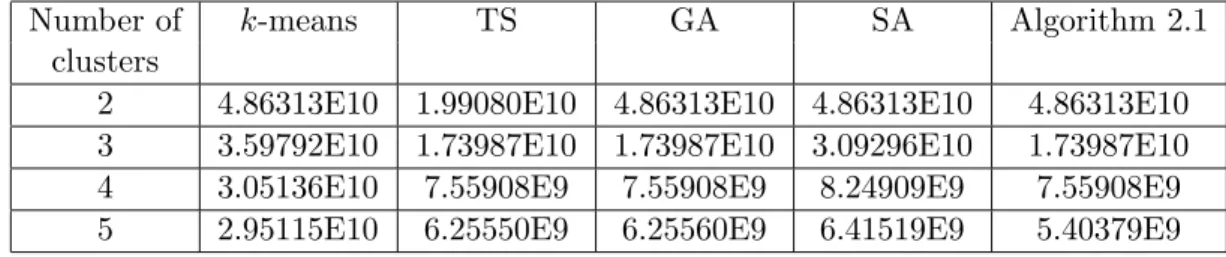
Table 3: Results for the second Bavarian postal zones dataset.
Number of k-means TS GA SA Algorithm 2.1
clusters
2 4.86313E10 1.99080E10 4.86313E10 4.86313E10 4.86313E10 3 3.59792E10 1.73987E10 1.73987E10 3.09296E10 1.73987E10 4 3.05136E10 7.55908E9 7.55908E9 8.24909E9 7.55908E9 5 2.95115E10 6.25550E9 6.25560E9 6.41519E9 5.40379E9
The results presented in Table 3 show that for this dataset, Algorithm 2.1 achieves better results than the k-means algorithm. Moreover this algorithm gives the best results for k = 3,4,5.
Based on the results presented in Tables 1-3 we can conclude that at least for these three datasets, Algorithm 2.1 works better than the k-means algorithm and achieves close, similar and sometimes better results than tabu search, genetic and simulated annealing algorithms, using significantly less CPU time. These results confirm that the proposed algorithm, as a rule, finds “deep” local minima or sometimes a global minimum of the objective function in a clustering problem.
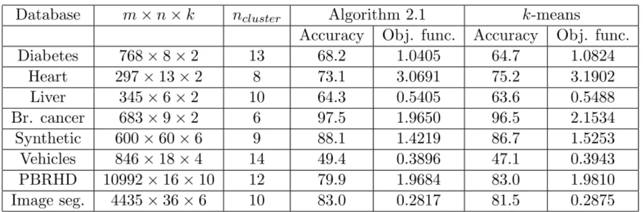
Finally, we applied our algorithm to calculate clusters in some databases with known classes. We used the diabetes, liver disorder, heart disease, breast cancer, vehicles, synthetic, pen-based recognition of handwritten digits (PBRHD) and image segmentation datasets in nu-merical experiments. Descriptions of these datasets can be found in Appendix.
First, we normalized all features. This was done by a nonsingular matrix so that mean values of all features were 1.
we applied Algorithm 2.1 to calculate clusters. Then the k-means algorithm was applied with the same number of clusters as calculated by Algorithm 2.1.
Results of the numerical experiments are given in Table 4. In this table we present the characteristics of a dataset where m is the number of instances, n number of attributes (features), k the number of classes. We also present the accuracy and the value of objective function achieved by Algorithm 2.1 and k-means. In situations where instances are already labelled, we can compare the clusters with the “true” class labels. We use the notion of cluster
purity defined in [38] as:
P(C) = 1 nC max i=1,...,l n i C
to evaluate accuracy. In this expression nC =|C|is the cardinality of the clusterC,niC is the number of instances in the cluster C that belong to class i andl is the number of classes.
Table 4: Results of clustering in databases with known classes Database m×n×k ncluster Algorithm 2.1 k-means
Accuracy Obj. func. Accuracy Obj. func. Diabetes 768×8×2 13 68.2 1.0405 64.7 1.0824 Heart 297×13×2 8 73.1 3.0691 75.2 3.1902 Liver 345×6×2 10 64.3 0.5405 63.6 0.5488 Br. cancer 683×9×2 6 97.5 1.9650 96.5 2.1534 Synthetic 600×60×6 9 88.1 1.4219 86.7 1.5253 Vehicles 846×18×4 14 49.4 0.3896 47.1 0.3943 PBRHD 10992×16×10 12 79.9 1.9684 83.0 1.9810 Image seg. 4435×36×6 10 83.0 0.2817 81.5 0.2875
The results presented in Table 4 show that Algorithm 2.1 gives better results for all datasets, except the vehicles dataset where the results are almost similar. We can see that, as a rule, the smaller the value of the objective function the better the description of the dataset. However, this is not true always but in these cases the difference is very small. Note that the values of the objective function appearing in the table are given after scaling and dividing by the number of instances. The effect of this is that the actual differences are much larger than appearing in the table.
Remark 2.1 Often it is implicitly assumed that classes coincide with some clusters (or the union of some clusters) in all datasets with known classes. Of course this is only an assumption that should be checked. For some datasets the accuracy of the results of clustering in Table 4 are not very high, which shows that there is now straightforward relation between classes and clusters in these datasets. We shall explain this situation later on (see Subsection 3.10).
2.7 The k-means algorithm and the minimization of the cluster function
Most local methods are very sensitive to the choice of the initial point. In some cases it is reasonable to consider the result, obtained by one local method, as the initial point for another one. Since the k-means method is very fast, very often it used for initialization
Table 5: Medium-size datasets: k-means and optimization Dataset Clusters Features k-means Optimization
4 1-18 1996 1814 Vehicle 15 1-18 1458.8 1293.8 15 3,4,6-8,11,12,15,16 997 933.66 15 3,6-8,12,15,16 869 822.6 6 1-6 494 456 Liver 6 1-5 352 294 disorder 8 1-6 1735 497 4 1-6 1735.3 614.7 6 1-8 1820 1737 Diabetes 8 1-8 1709.56 1585 4 1-8 2047 1908 6 8,9,14 708.7 493 Australian 4 8,9,14 958.5 669 credit 4 1-14 5754 4743 4 2,3,5,7,8,13,14 3257 2610 6 2,3,5,7,8,13,14 2496 2231
of more computationally expensive methods. We consider a combination of k-means with non-smooth local optimization (Discrete gradient method, see Section 4).
For testing the efficiency of the combination of k-means and Discrete Gradient method, we use four well-known medium-size test datasets: Australian credit dataset, Diabetes dataset, Liver disorder dataset and Vehicle dataset. The description of these datasets can be found in Appendix. We studied these datasets, using different subsets of features and different numbers of clusters and without any division of them into classes.
We calculated the value of the cluster function for initial points x obtained by the k-means algorithm and then for the points ¯x obtained by Discrete Gradient method starting from x. The results are shown in Table 5. The second column in this table shows the number of clusters, the features, which are taken into account, are included in the third column, the 4th and 5th columns contain values of cluster function corresponding to points x found by
k-means (4th column) and points ¯x obtained by Discrete Gradient method starting from x
(5th column). We used either all features or some subsets of features that were found by the feature selection procedure, that is described in Subsection 3.3.
We came to the conclusion, that the combination of the k-means method and the Discrete Gradient method often works efficiently and produces better results than thek-means method only. Sometimes this improvement is not so significant, but for the liver disorder dataset (8 clusters and 4 clusters) and the Australian Credit dataset (6 clusters with features 8,9,14) this improvement is good enough.
We also considered the continuation of this process. We ran thek-means method from the ini-tial point, obtained after the nonsmooth optimization method. Empty clusters appeared after the second iteration, and the results were not so good. So, for the medium-size datasets under consideration we found, that it is reasonable to make only one iteration for the combination method.
2.8 Clusters and their structure
A cluster with known centre xj can be described as the set of points a∈A such that
kxj −ak ≤min i6=j kx
i−ak. Consider points a∈Asuch that
kxj−ak ≤cmin i6=j kx
i−ak
where c > 0. If c is small enough then we can assign a to the cluster j with the greater confidence. Let φj(a) = min{c >0 :kxj−ak ≤cmin i6=j kx i−ak}, µj(a) = 1 1 +φj(a) . Then 0< µj(a)≤1, µj(a) = 1 ⇐⇒ a=xj, µj(a)≥1/2 ⇐⇒ kxj −ak ≤min i6=j kx i−ak.
We can considerµj as a membership function for the fuzzy clusterj. Thus each point belongs to each cluster in a fuzzy sense. Clearly if µj(a) is closer to one then the confidence that a belongs to the cluster j is greater.
For a better understanding of the structure of the cluster j we need to consider the sets
{a∈A:kxj−ak ≤clmin i6=j kx
i−ak}
with different cl≤1 (for examplecl = 1,0.9,0.8, . . . ,0.1.) Often these sets with small enough cl are either empty or “almost empty”. This can be interpreted in the following way: the cluster j is located in a certain ring; there are (almost) no points of this cluster, which are close to its centre. We can describe this situation by saying that the cluster is concentrated in its periphery and sparse and its centre. Points, which are in the outer periphery, can be considered as questionable. A change of the norm is more likely to lead to the change of the membership for these points.
We can use the structure of clusters in order to estimate the quality of a given candidate
X = (x1, . . . , xn) as the centres of clusters. The candidate X
∗ is more appropriate than X, if clusters corresponding to X∗ are more concentrated in the vicinity of their centres. This approach is a complementary to the estimation of centres of clusters by means of cluster function.
The results of numerical experiments demonstrate that the minimization of the cluster func-tion with initial points obtained byk-means algorithm often improves the structure of clusters. We considered the following datasets: emergency, pen-based recognition of handwritten dig-its, image segmentation and letters dataset (see Appendix for their description). We found the clusters within the datasets without any division into classes. We present here one of the brightest examples (for Emergency dataset with 7 clusters). We used the normk · k1.
Table 6: Emergency dataset. k-means algorithm. c 1 0.9 0.8 0.7 0.6 0.5 0.4 0.3 0.2 0.1 cluster I 7727 7379 6981 6429 5861 4553 2679 702 18 0 cluster II 471 435 389 330 266 191 103 39 5 0 cluster III 1113 956 781 592 409 235 95 18 1 0 cluster IV 1611 1401 1215 980 695 443 226 61 9 0 cluster V 803 691 584 477 328 200 100 43 4 0 cluster VI 92 88 79 73 68 56 44 26 8 1 cluster VII 3369 2928 2464 1869 1330 799 265 59 1 0 Table 7: Emergency. Discrete gradient algorithm.
c 1 0.9 0.8 0.7 0.6 0.5 0.4 0.3 0.2 0.1 cluster I 4034 3612 2892 2188 1975 1741 1499 1202 777 174 cluster II 921 847 759 614 429 288 183 92 27 12 cluster III 2901 2478 2060 1651 1238 922 701 438 169 14 cluster IV 1584 1372 1194 987 725 496 316 179 76 5 cluster V 1966 1737 1451 1114 785 528 302 146 48 4 cluster VI 123 112 101 94 88 76 56 39 11 2 cluster VII 3657 3268 2477 2067 1849 1559 1290 932 527 111
In Table 6 and Table 7 we present the structure of clusters, obtained by the k-means method and the nonsmooth optimization algorithm, respectively. An initial point for optimization is the set of centers of clusters that were found by the k-means method.
Notice that the Discrete gradient algorithm reached another location for the centres. Many points within the clusters moved from the periphery of the clusters to their centres. The value of the objective function, multiplied by the number of points in dataset was decreased from 22446.3 to 19408.4.
2.9 Generalized cluster functions and complexity reduction for large-scale datasets
Due to the highly combinatorial nature of clustering problems, two characteristics of a given dataset can severely affect the performance of a clustering tool: the number of data records (instances) and the number of data attributes (features). In many cases the development of effective tools requires the reduction of both the number of features and the number of instances without loss of knowledge generating ability. We firstly consider the reduction of the number of instances. The reduction of the number of features will be discussed later on (See Subsection 3.3 and Subsection 3.4).
Large-scale datasets usually contain a huge number of points located in a bounded set. Thus many points from this dataset are very close to each other. Let A ⊂ IRn be a finite set. Assume that a certain small neighborhood of a point b∈IRn contains mb points from A. We can approximate each of these points by b and replace the corresponding part of the cluster function by the simple term mbminikxi−bk.
for each a ∈ A there exists b ∈ B with the property ka−bk < ε. We say that a collection (Ab)b∈B of subsets of A is anε-disjoint cover of A if
ka−bk< ε, (a∈Ab), Ab∩Ab0 =∅(b6=b0), A= [
b∈B Ab.
Let mb be the cardinality of Ab. Replacing each a ∈ Ab with b in the presentation of the cluster functionCk we obtain the following function
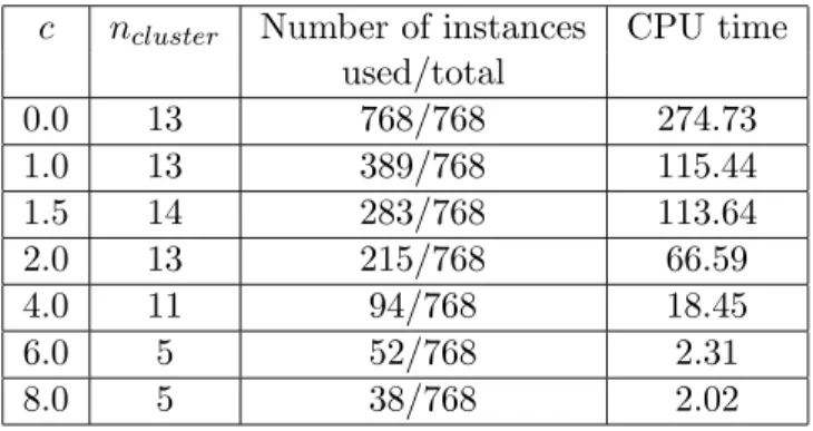
˜ Ck(x1, . . . , xk) = 1 m X b∈B mbmin(kx1−bk, . . . ,kxk−bk), which will be called the generalized cluster function.
-30 -20 -10 10 20 30 82.5 87.5 90 92.5 95
Figure 3: Generalized cluster function in IR1
Figure 3 illustrates a plot of a function of one variable f(x) = ˜C2(x,x¯2) with fixed ¯x2, where ˜
C2 is a generalized cluster function in IR1 for a dataset with 23 points.
We shall use generalized cluster functions for the approximation of cluster functions. Since the notion of cluster is flexible, we can consider an appropriate approximation of the cluster function, which can even be not very exact. The following assertion holds (see [77]).
Proposition 2.1 Let (Ab)b∈B be an ε-disjoint cover of A and C˜k be the generalized
clus-ter function corresponding to this cover. Then |Ck(x1, . . . , xk)−C˜k(x1, . . . , xk)| < ε for all (x1, . . . , xk)∈(IRn)k.
Proposition 2.1 allows us to substitute the given dataset A for a smaller dataset B. The minimization of the generalized cluster function ˜Ckcorresponding to this set will give us some points (x1, . . . , xk). We can consider these points as centres ofkclusters of the setA. Then a cluster Aj corresponding to centrexj can be described as the union of setsAb over allbsuch that kb−xjk ≤mini6=jkb−xik.
We now suggest a simple scheme for the construction of an ε-disjoint cover of A with the given tolerance ε. Let A={ai}i=1,...,m be a given dataset. (Such a representation of the set
A means that we consider this set with a certain order relation: for each point a ∈ A we indicate its number. The procedure described below depends on the order relation given on the set A. However, as was found from calculations, this dependance is not significant.) Let D = (dij))i,j=1,...,m be a symmetric matrix with dij = kai−ajk. We shall consider the following procedure: select the first vector a1, remove from the dataset all the vectors for which d1j ≤ε, and assign to this vector the numberm1 of removed vectors. Denote a1 =b1. Then select the next remaining vector b2 and repeat the above procedure for this vector,etc. As the result of this procedure we get a subset B = {bj}l
j=1 of the given set A and the set (mj)lj=1, wheremj is the number of removed vectors at the stepj. The cardinalitylofB can be significantly less then the cardinality m of A. For the search for clusters of the set A we shall apply the generalized cluster functions
˜ Ck(x1, . . . , xk) = 1 m l X j=1 mjmin(kx1−bjk, . . . ,kxk−bjk).
In this scheme a selected vector bj serves as the representative of the set Aj of all points removed at the step j.
Remark 2.2 Different versions of this approach are also possible. For example we can use a point bj only for the determination of the set Aj. The centroid of this set can be chosen as its representative.
For implementation of the scheme under consideration we need to suggest an appropriate choice of the tolerance ε. We consider two different approaches to this choice.
2.10 Complexity reduction for large-scale datasets: first approach
For each i, i= 1, . . . , m, calculate
ri = min j6=i dij, where dij =kai−ajk. Let r0 = 1 m m X i=1 ri. Select ε=cr0 with c >0.
The results of numerical experiments reported below suggest that such a procedure allows one to significantly reduce the number of instances in the dataset.
In this scheme a key element is the choice of the parameter c. We can give some recom-mendations on the choice of this parameter using the results of numerical experiments. The dependence of the number of clusters on this parameter can be studied and we use three databases: diabetes, heart disease and liver disorder databases in numerical experiments. The description of these databases can be found in the Appendix. We applied the Algorithm 2.1 to the entire dataset without dividing it into classes. We took the tolerance εfrom Step 3 in Algorithm 2.1 equal to 10−2 and repeated the computations for differentc. Results of numerical experiments are given in Tables 8-10. In these tables we present the number of clus-ters ncluster calculated by the algorithm, the number of instances remained after application of the scheme for particular value of the parameter c and CPU time.
Table 8: Results of numerical experiments for the diabetes database
c ncluster Number of instances CPU time used/total 0.0 13 768/768 274.73 1.0 13 389/768 115.44 1.5 14 283/768 113.64 2.0 13 215/768 66.59 4.0 11 94/768 18.45 6.0 5 52/768 2.31 8.0 5 38/768 2.02
The results presented in Table 8 show that for the diabetes dataset we can take c ∈ [0,4]. Further decrease of c leads to sharp changes in the cluster structure of the dataset. We can see that there are differences in the number of clusters whenc∈[0,4]. But forc∈[0,2] these differences arise because of small clusters. We can also see that for c∈[1.5,4] the number of instances and CPU time reduce significantly.
Table 9: Results of numerical experiments for the heart disease database
c ncluster Number of instances CPU time used/total 0.0 8 297/297 75.59 1.0 7 152/297 26.73 1.5 6 122/297 14.43 2.0 5 107/297 8.25 4.0 5 65/297 5.05 6.0 5 41/297 3.34 8.0 5 28/297 3.22
The results presented in Table 9 show that appropriate values for the heart disease dataset are c ∈[0,1.5], because further decrease in c leads to changes in the cluster structure of the dataset. We can again see that these values of c allow significant reduction in the number of instances and CPU time.
From the results presented in Table 10 we can conclude that appropriate values of c for the liver disorder dataset are c∈[0,2]. Differences in the number of clusters whenc∈[0,2] arise because of small clusters which contain less than 5 % of all instances.
Thus using results of numerical experiments on these three datasets we can conclude that appropriate values for the parameter c arec= 0∈[0,2] and preferable values are c∈[1.5,2] because in the latter case we can remove the maximum number of instances from a dataset without serious changes in the cluster structure of the dataset.
Table 10: Results of numerical experiments for the liver disorder database
c ncluster Number of instances CPU time used/total 0.0 10 345/345 57.66 1.0 12 129/345 37.48 1.5 11 97/345 24.95 2.0 13 79/345 37.16 4.0 8 43/345 4.33 6.0 7 34/345 3.13 8.0 7 29/345 2.67
2.11 Another approach to complexity reduction for large-scale datasets
Let ε be a given tolerance. Proposition 2.1 shows that the generalized cluster function ˜Ck approximates the cluster functionCkwith the absolute errorε. Since we are mainly interested in the relative error, it is appropriate to choose ε=εh where
εh =hCk(x1, . . . , xk)
and x = (x1, . . . , xk) is a point close enough to a global minimum. We can choose x as the result of thek-means algorithm starting from a certain initial point. The procedure with such a choice of εh will be called theεh-cleaning procedure.
Numerical experiments have been carried out with some datasets of medium size and large-scale datasets. We give here only results for the liver disorder, diabetes and heart disease datasets (Table 11) and emergency dataset (Table 12). Descriptions of all these datasets can be found in the Appendix. Here we consider the centroid of the class of the removed points as its representative. (See Remark 2.2.) We use the combination of k-means with the Discrete Gradient method for the minimization of the generalized cluster function. We also use both norms k · k1 and k · k2. Different norms give different results but they are quite comparable. The following observation is of a certain interest. Assume that one of the norm k · k1 ork · k2 is fixed and a set of centers of clusters y = (y1, . . . , yk) is found by the k-means algorithm starting from a point x= (x1, . . . , xk). Let Ck be the cluster function with respect to either
k · k1 or k · k2 (this does not depend on the fixed norm). Applying the Discrete Gradient algorithm with the initial pointy for minimization ofCk we can find a pointz= (z1, . . . , zk). We considered many initial points x and could not find an example where the inequality
Ck(x)> Ck(y)> Ck(z) does not hold, even if the norms, which was used for k-means and for the definition of Ck, did not coincide.
In the Table 11 we present results for both norms and only for one tolerance εh. In the Table 12 we present results only fork · k1 with differentεh. The results obtained for different number of clusters 2 ≤k≤10 are similar, so we present the results only for k= 7. We ran the programs with different εh in order to find the tolerance which allows reduction of the number of observations and keeps the approximation of the cluster-function reasonable. In both tables the column Size describes the size of the dataset after εh−cleaning. The columnDistancecontains the information about the differencedh between centres of clusters
Table 11: Choice ofεand clustering. Medium size datasets. 4 clusters. Dataset Norm h Size Distances Change of clusters
Liver (345) 1 0.9 133 0.73 0, -0.057, -0.079, 0.081 Liver (345) 2 0.9 78 0.61 0,075, -0.077, -0.032, 0.013 Diabetes (768) 1 0.6 290 1.46 -0.047, 0.075, -0.004, 0.008 Diabetes (768) 2 0.6 200 1.59 0.102, 0.042, -0.018, 0.138 Heart (297) 1 0.9 57 3.87 0, -0.027, 0.036, -0.010 Heart (297) 2 0.9 106 0.48 0, 0, 0, 0
Table 12: Choice of εand clustering. Emergency dataset.
h Size Distance Change of clusters
0 15 186 0 0, 0, 0, 0, 0, 0, 0 0.1 5989 1.09 0.009, -0.102, 0.009, -0.021, 0.009, 0.024, -0.09, -0.007 0.2 2740 1.00 -0.010, 0.007, 0.012, 0.011, -0.025, 0.008, 0.009 0.3 1487 1.07 0.075, -0.035, -0.009, 0.008, 0.158, -0.049, -0.153 0.4 938 1.53 -0.390, 0.150, 0.255, -0.016, 0.302, 0.098, -0.032 0.5 652 2.32 -0.289, 0.238, 0.165, 0.017, 0.340, 0.139, -0.066
with and without εh-cleaning: dh = 1kPki=1kx¯i −x¯ihk. Here k is the number of clusters; ¯xi are the centres of clusters of the original dataset, obtained by the minimization of the cluster function, and ¯xih the centers obtained by the minimization of the generalized cluster functions corresponding to εh. The column Change of clusterscontains the numbers Rih, i = 1, . . . , k that characterize the change of the size of each cluster. By definition
Rhi = Nor−N i clear Ni or ,
where Nori is the number of points within the cluster i, that obtained by the minimization of the cluster function, and Ncleari is the number of points within this cluster, obtained by the minimization of the generalized cluster functions. Table 11 contains also the columns
Dataset, where the name of the dataset and its size (in brackets) are shown and the column
N orm.
Table 12 demonstrates that even reducing the size of the Emergency dataset by more than 10 times we get satisfactory results. The obtained results also show that even very rough approximation of the cluster function leads to satisfactory results.
Comparing Table 11 and Table 12 we can suggest that the percentage of points that can be removed without destroying the structure of datasets heavily depends on the size of the dataset under consideration: for a larger dataset this percentage is bigger. Indeed, it follows from the following simple observation: if two datasets are located in the same volume then points from a larger dataset are closer to each other. This conclusion allows us to hope that
εh cleaning procedure can be successfully used for clustering very large datasets.
The following conclusion is also of interest. Two different approaches to choosing ε: the first approach is based on the minimal distance between the points and the second one controls the relative error left almost the same number of points after “cleaning”.
2.12 Geometry of finite sets
Clusters can describe the structure of finite sets of points. It is important also to describe some different characteristics of finite sets, which can help in the study of these sets and also classification problems related to them. We give an example of such characteristics (see [79] for details).
Example 2.1 Let A be a finite set of points. We describe this set by a collection of hyper-planes.
Consider vectors l1, . . . , lk withklik= 1 and numbersbi (i= 1, . . . , k). LetHi={x: [li, x] = bi} and H = ∪iHi. Then the distance between the set Hi and a point aq is d(aq, Hi) =
|[li, aq]−bi|and the distance between the set H and aq is d(aq, H) = min
i |[li, a q]−b
i|. The deviation of X from A is
X q∈Q d(aq, H)≡X q∈Q min i |[li, a q]−b i| Consider the function
Lk((l1, b1), . . . ,(lk, bk)) = X q∈Q min i |[li, a q]−b i|. A solution of the following constrainedmin-sum-min problem
min (l1,b1)∈IRn+1,...,(lk,bk)∈IRn+1 X q∈Q min i |[li, a q]−b i| subject to kl1k= 1, . . . ,klkk= 1
describes theskeleton of the set A, which is formed byk hyperplanes.
It is easy to give some examples of finite sets, for which skeletons are a better description of the set than clusters. Skeletons can also find some applications in classification.
3
Supervised classification via clustering
3.1 Introduction
The aim of supervised data classification is to establish rules for the classification of some observations assuming that the classes of data are known. To find these rules, an investigator can use known training subsets of the given classes. The construction of a classification pro-cedure may also be a pattern recognition propro-cedure, a discrimination propro-cedure or supervised learning procedure. Those problems arise in a wide range of human activity.
There are many methods for data classification, which are based on quite different approaches (statistics, neural networks, methods of information theory etc). Excellent review of these
approaches, including their computational investigation and comparison, can be found in [67]. Statistical approaches to classification are described in [64].
One of the most promising approaches to data classification is based on methods of mathe-matical optimization. For supervised classification, where we have a database, which consists of at least two classes and there is a training set for each class, there are two different ways for the application of optimization. The first, which we shall callouter, is based on the separation of the given training sets by means of a certain (not necessary linear) function. The outer approach is currently the most popular. (See, for example, [28, 29, 63], where problems of quadratic and bilinear programming are used for classification and then linear programming techniques are applied for the solution of these problems.) The second (inner) approach con-sists of describing clusters for the given training sets. The data vectors are assigned to the closest cluster and correspondingly to the set, which contains this cluster. The description of this approach can be found in the recent paper [18]. Numerical experiments demonstrate that for supervised classification of databases of a small to medium size, the inner approach gives a more precise description of databases than the outer approach. We examine the inner approach in this section. For the implementation of this approach one needs to solve a com-plex problem of nonsmooth and nonconvex unconstrained optimization, either local or global. In spite of the nonsmoothness and nonconvexity of the objective function, local methods are much simpler and more applicable, than global ones.
On the other hand global methods give more precise descriptions of clusters. A deterministic method for solving global optimization problems (the cutting angle method) has recently been developed [6, 19, 20, 23]. Some modifications of the cutting angle method and its combination with a local search ([21]) were successfully applied to classification. Our numerical experiments with real-world databases of small to medium size show that the inner approach to the supervised classification problem based on optimization techniques gives results close to the best known ones obtained by different methods. (see Section 3.8).
3.2 The inner approach to classification
Assume that we have a dataset consisting of l classes A1, . . . , Al. Assume that the class Aj consists of kj clusters. We can use the minimization of the cluster function Ckj in order to
find centers of these clusters and then use these clusters for classification. From the first view this approach is not suitable. Indeed, actually we reduce the more simple problem of super-vised classification to the series of more complicated problem of unsupersuper-vised classification. However, the presence of known classes substantially facilitates the search for clusters. The cluster function Ck depends on n×k variables, where n is the number of attributes (features) and k is the number of clusters. If classes are known, we can apply a certain feature selection procedure (see Subsection 3.3) for diminishing the number of features, hence we can use only n1 < n features. Second, we can determine the centers of clusters step by step. This means that we consider a series of k problems of the dimension n1 instead of one problem of the dimension n1×k. The solution of this series is much easier then solving one high-dimensional problem. We now explain why step by step procedure can be used for supervised classification.