Adjoint-Based Aerodynamic Optimisation of Wing Shape Using Non-uniform Rational B-Splines

Wing Shape Using Non-Uniform Rational

B-splines

Xingchen Zhang, Rejish Jesudasan and Jens-Dominik M¨uller

Abstract Numerical shape optimisation with adjoint CFD is applied using the NURBS based Parametrisation method with Continuity Constraints (NSPCC) for aerodynamically optimising three dimensional surfaces. The ONERA M6 wing is re-parametrised with NURBS surfaces including weight adjustments to repre-sent the three dimensional wing accurately, resulting in fewer control points and smoother variation of curvature. The NSPCC CAD kernel is coupled with the in-house flow and adjoint solver STAMPS and a gradient-based optimiser to minimise the drag of the ONERA M6 wing in transonic Euler flow conditions. Optimisation results are presented for the B-Spline and NURBS parametrisations.

1 Introduction

Numerical shape optimisation has attracted widespread interest in recent years. This is mainly driven by engineering design facing ever-increasing requirements in per-formance, environmental impact and life-time cost. To satisfy these needs, large design spaces with many degrees of freedom need to be explored systematically, which can only be achieved through numerical optimisation.

Gradient-free optimisation methods such as Genetic Algorithms (GA) or Evo-lutionary Algorithms (EA) are very established, especially for linear structural

op-Xingchen Zhang

School of Engineering and Materials Science, Queen Mary University of London, Mile End Road, London, E1 4NS, UK e-mail: [email protected]

Rejish Jesudasan

School of Engineering and Materials Science, Queen Mary University of London, Mile End Road, London, E1 4NS, UK e-mail: [email protected]

Jens-Dominik M¨uller

School of Engineering and Materials Science, Queen Mary University of London, Mile End Road, London, E1 4NS, UK e-mail: [email protected]

timisation where the computational cost of an evaluation is low. However, these methods require a large number of function evaluations when going beyond 50-100 design variables, and this cost becomes prohibitive when used with expensive CFD models.

The convergence of gradient-based methods on the other hand suffers much less from large design spaces and they have been adopted as the method of choice for shape and topology optimisation with CFD. This replaces the hurdle of computa-tional cost with the challenge to compute the gradients for all components in the simulation chain, i.e. not only the flow solver, but also the parametrisation. Gradient computation can be easily implemented using finite differences, however this incurs truncation or round-off errors that can be difficult to control. Alternatives are the complex step method [1] or algorithmic differentiation [2, 3] which can produce ex-act derivatives, but the computational cost scales linearly with the number of design variables. The adjoint method allows to compute the gradients of an objective with respect to an arbitrary number of design variables at constant cost and has hence be-come the method of choice in CFD [4, 5]. However, implementing an adjoint solver is not trivial, both the continuous approach [6] as well as the discrete one [7, 8, 9] require a significant effort.

One of the key issues in shape optimisation is the parametrisation of the geom-etry, because it will determine the design space and thus the optimisation result. Current parametrisation methods can roughly be distinguished as CAD-free and CAD-based ones. In the CAD-free approaches, the parametrisation has no link back to the CAD geometry, which makes these approaches easy to implement. Examples are mesh deformation through Radial Basis Functions [10], Free-form Deformation with volume splines [11] and node-based approaches [12, 13, 14]. The downside of these approaches is that at the optimal result needs to be transcribed back to CAD which is often cumbersome and may lose relevant features of the optimised shape.

In CAD-based methods, the parametrisation of the shape is part of the CAD model which is kept inside the design loop. Hence the resulting optimal shape is directly available for further analysis or manufacturing. The main difficulty for gradient-based optimisation is that we also need to compute derivatives of the para-metric CAD model.

The parametrisation can be defined explicitlyin a parametric CAD system, as often done to generate a family of parts in different sizes or for manual design space exploration. While this approach has the advantage that geometric constraints such as thicknesses or radii can be directly built into the design space, typically these parametrisations either do not have sufficient freedom to capture relevant modes, or require important human knowledge about the flow and incur significant user effort to set up, which ultimately negates the benefits of numerical optimisation. Derivative computation of the explicitly parametrised CAD model can then either through finite-differencing, which incurs the typical problems of finite differences with truncation errors and choice of step size. Robinson et al [15] avoid problems of robustness due to patch renumbering by approximating the surfaces with triangula-tions (STL), which in turn has issues with projection near sharp corners.

Gradients can also be computed by applying automatic differentiation to the source code of the CAD system, which addresses issues of accuracy and will al-low use of the efficient reverse mode [16]. This approach still requires to define a suitable CAD parametrisation.

Alternatively, a CAD-based parametrisation can also be definedimplicitly, i.e. to arise from the CAD model’s generic description such as the collection of NURBS patches in the STEP or IGES standards. The positions and weights of the control points (CP) of the NURBS patches can be used as design variables.

In this work, the QMUL in-house CAD kernel, termed NURBS-based parametri-sation with continuity constraint (NSPCC) [17, 18] is used to parametrise the geom-etry, and is integrated into the CAD-based optimisation loop. This approach offers a number of advantages. Firstly only a subset of CAD functionality is needed which can straightforwardly be implemented in light-weight standalone tools, which in turn significantly simplifies the derivative computation with automatic differentia-tion tools [17]. Secondly the implicit parametrisadifferentia-tion through control points typi-cally produces a suitably rich design space without need for manual setup [19]. On the downside, a methodology needs to be introduced for imposition of geometric constraints, such as continuity constraints between NURBS patches or thickness, box and radii constraints. This can be achieved effectively with a test-point method-ology [17, 20]. The design space is in most cases excessively rich, however when using the adjoint approach to evaluate the gradients, this is not an inconvenient. Pro-vided that the design space remains coarser than the CFD mesh, gradient regularisa-tion is not required, as opposed to mesh-based parametrisaregularisa-tions [12]. However, rich design spaces may lead to shapes with mildly oscillatory modes that are not detri-mental to the objective function, hence not penalised by the flow solver, but may be undesirable as they are visually unappealing or affect another discipline/behaviour that is not modelled. This aspect is addressed in this paper.

In this paper we will present a methodology that uses as free parameters not only the positions of the NURBS control points, but also their weights. This enables to ac-curately represent shapes with coarser control lattices, resulting in smoother changes of curvature which can be important in the design of turbo-machinery blades or tran-sonic wings.

The remaining part of this paper is structured as follows: Section 2 introduces the adjoint approach briefly, then Sec. 3 provides information on NURBS and also the NSPCC approach. The approximation of ONERA M6 wing using NURBS will be presented in Sec. 4, followed by the optimisation results in Sec. 5. Finally, the conclusion will be given in Sec. 6.

2 Adjoint approach

Let us consider the Navier-Stokes equations as

whereRis the conservative residual of flow equations,Uare state variables andaaa

is a set of design variables. Taking the derivative of (1) with respect toaaa, we have:

∂R ∂U ∂U ∂aaa+ ∂R ∂aaa =0, (2)

which can be written as

Au=f, (3)

whereAis the Jacobian ∂_∂R_U,uis the perturbation field, i.e. the change of the flow field with respect toaaaandfis the change in residual w.r.t changes in shape,∂R

∂aaa.

The sensitivity of the objective functionJwith respect to the design variablesaaa

can then be formulated as: dJ daaa = ∂J ∂aaa+ ∂J ∂U ∂U ∂aaa = ∂J ∂aaa+gTu, (4) wheregT₌ ∂J

∂U. In (4), the computation of the partial derivative∂aaa∂J is not expensive.

Similarly, the source term f in (3) is computationally inexpensive, but depends on the design variableai. However computinguinvolves solving a linear system solve

for each componentaiofaaa, a cost which will become prohibitive if the number of

design variables is large.

On the other hand, the sensitivity of the objective dJ

daaa can be obtained without

computing the perturbation fielduwith the adjoint method. Using the solution of (3),u=A 1f, in (4) and transposing one obtains

dJ daaa T =_∂aaa∂J T + (gTA 1f)T =_∂aaa∂J T +fTA Tg (5) By transposing the second term on the right hand side, we have:

fT_A T_{g (6)}

The right-most matrix-vector productA T_{gcan be interpreted as a linear equation}

similar to equation (3) for a new variablev,

AT_{v=g. (7)}

With a solution for the adjoint variablevwe can rewrite (5) as dJ

daaa = ∂J

∂aaa+vTf. (8)

The adjoint equivalence then states

gT_{u= (A}T_v)T_u=vT_Au=vT_{f. (9)}

Since the adjoint variablevdepends only on the flow field through the transposed JacobianAT_{and on the objective throughg, (8) allows to compute the entire}

sensi-tivity vector _daaadJ with a single system solve of (7). Hence the cost of computing the gradient becomes independent of the number of design variables.

Using the chain rule of calculus, the differentiation of the objective function can be broken down into a number of steps, aligned with the computational workflow,

∂J ∂aaa = ∂J ∂xV ∂xv ∂xs ∂xs ∂aaa (10)

with the volume grid coordinatesxV, which in turn are linked to perturbations of

the surface grid coordinatexBthrough a mesh deformation algorithm, which in turn

are affected by modifications of the CAD parametersaaa. The first term on the right hand side∂J/∂xVis computed by differentiating the flow solver, the second term

∂xv/∂xs by differentiating the the volume mesh smoothing, while the third term

∂xs/∂aaarequires a differentiation of the CAD model parametrisation.

In our work we employ Automatic Differentiation (AD) Software tools Tapenade [21] to produce the adjoint code and assemble the routines in a hand-written driver code to improve performance [9].

3 Parametrisation

Parametrisation of geometry is crucial in shape optimisation as it will affect the design space. There are various parametrisation methods which can generally be distinguished as CAD-free and CAD-based methods. In this work, we focus on the CAD-based approach using boundary representation (BRep), where NURBS is the standard way to express geometries.

3.1 NURBS surface patches

Non-Uniform Rational B-splines (NURBS) are widely used to describe geometries. A NURBS patch is a 3D surface defined as [22]:

S(u,v) = n  i=0 m  j=0Ni,p(u)Nj,q(v)wi,jPi,j n  i=0 m  j=0Ni,p(u)Nj,q(v)wi,j 0u,v1 (11)

where Pi,j are the control point coordinates, wi,j their corresponding weights,

Ni,p(u)andNj,q(v)thep-th andq-th degree B-spline basis functions defined in the

following knot vectors: {0, . . . ,0 | {z } p+1 ,up+1, . . . ,ui, . . . ,ur p 1,1, . . . ,1 | {z } p+1 }

{0, . . . ,0 | {z } q+1 ,vq+1, . . . ,vj, . . . ,vs q 1,1, . . . ,1 | {z } q+1 }

wherer=n+p+1 ands=m+q+1.Ni,p(u)andNj,q(v)are given by the following

expression: Ni,0(u) = ⇢ 1i f uiu<ui+1 0otherwise Ni,k(u) =_u(u ui) i+k uiNi,k 1(u) + (ui+k+1 u) ui+k+1 ui+1Ni+1,k 1(u) (12)

NURBS hold many geometric properties, making them very suitable to describe geometries in shape optimisation problems. Some of them are:

• Local modification. If a control point is perturbed, only a part of the geometry will be affected.

• Generalisation. NURBS can be used to describe very wide range of geometries, including circular and conic shapes, which the B-splines can not express exactly. • Strong convex hull property.

• Affine invariance.

A NURBS surface can be expressed in the so-called homogeneous form:

Sw(u,v) = n

Â

Â

Ni,p(u)Nj,q(v)Pwi,j 0u,v1 (13)

wherePw

i,j= (wi,jxi,j,wi,jyi,j,wi,jzi,j,wi,j). This homogeneous form is very similar

to a spline surface, therefore if written in this form, most of the algorithms for B-spline surfaces can straightforwardly be applied to NURBS. In this way, the weights can also be used in shape optimisation problems.

3.2 NSPCC approach

NSPCC is an in-house lightweight CAD kernel, which uses an implementation in Fortran90 of NURBS patches which can then be differentiated using the source-transformation AD-Tool Tapenade [23]. Xuet al[17] considered B-splines and used the coordinates of the control pointsPi j to derive the design variables. Zhang et

al. [18] extended NSPCC from B-splines to NURBS and also include the weights

wi jin the design space.

The important contribution of NSPCC to CAD-based parametrisation based on the BRep is the formulation of geometric constraints, e.g. G0-G2 continuity at NURBS patch interfaces. The constraint equations are formulated numerically at a sufficiently large number of test-points [18] and the derivatives of these equations are computed using AD. The design space is the kernel of this matrix of constraint derivatives and is evaluated using singular value decomposition. The design vari-ables are ultimately the singular vectors of the SVD basis for the kernel. Details of

the NSPCC approach can be found in [17, 20]. Using the homogeneous form (13) then allows to extend the constraint framework straightforwardly from B-Splines to NURBS.

The scale and effect of the design variables will have a significant influence on the convergence toward the optimum. Considering e.g. a curve aligned with thex -axis. Control point movements in the curve-normaly direction will have a much stronger effect on the shape than movements in the tangentialx-direction. Simi-larly, the weights have scalings around unity, while the scaling of the coordinates entirely depends on the measurement units used for the coordinate values. In the NSPCC approach, the scaling strategy from [24] is applied to control points such that a variation of the scaled control points inxdirection between±1 causes around ±10% variation of the root chord length, and a variation of scaled control points in ydirection yields±10% deformation of the maximum thickness of root profile.

NSPCC uses the STEP file [25] as input and output for the geometry. The al-gorithm is hence independent of any internal proprietary parametrisation inside a particular CAD system.

4 M6 wing profile approximation using NURBS

The M6 wing [26] is a typical example of a geometry that cannot be represented ex-actly in CAD, hence defining a CAD model for the M6 requires a trade-off between fidelity and complexity. A similar case is the approximation of a cylindrical shape with B-splines, the standard choice for approximation in CAD systems. A low tol-erance of deviation between B-spline surface and the analytic cylindrical shape will result in a B-spline approximation with very many control points. On the other hand, a NURBS-representation allows to match a cylinder exactly with 6 distinct control points for a circular section. Lepineet al.[27] fitted NURBS to reduce the num-ber of control points for 2D aerofoils. In this work, we directly approximate the 3D wing shape with NURBS in the NSPCC framework. This has two major advantages. Firstly, even though the cost of computing the derivatives is constant with the ad-joint approach, the lower number of control points will make it easier for optimiser to converge the KKT system. Secondly, and more importantly, the smaller number of control points will result in a smoother variation of curvature along the profile, which is an essential quality in the design of transonic wings and turbomachinery blades.

As a first step, we compare the approximation of datum M6 wing shape using B-Spline and NURBS representations. The M6 wing created with 26 B-splines control points for each section (see Fig. 3) according to the description in [26] is used as the target shape [28, 29]. The wing parametrised with different numbers of NURBS control points are used as starting point. Then the cost function of this optimisation problem is defined as the root-mean-squared difference between initial and target geometries, i.e.:

J= s 1 N N

Â

whereXInitialiandXTargeti are surface points sampled on the initial and target wing

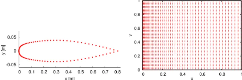
geometry, respectively.Nis the number of sample points. To improve the surface fidelity in regions of high curvature a cosine spacing as shown in Fig. 1 is used which concentrates the sampling points near the leading edge than near the trailing edge, as shown in Fig. 1.

-0.05 0 0.05 0 0.1 0.2 0.3 0.4 0.5 0.6 0.7 0.8 y [m] x [m] 0 0.2 0.4 0.6 0.8 1 0 0.2 0.4 0.6 0.8 1 v u

Fig. 1 Cosine spacing sample points. Left: points of one section. Right: points in parametric space.

For the M6 fitting in this study, 5000 surface points are sampled on each geome-try, 100 points in the chordwise and 50 points along the spanwise direction.

The initial wing geometries with different number of NURBS control points are driven towards the target shape by performing optimisation using the L-BFGS method [30, 31]. The gradients are calculated using AD, i.e. the derivative of the objective function w.r.t the design variables, i.e. the 2-D coordinates of the control points in the profile plane and their weights.

The objective function values (14) resulting from the optimisation with varying numbers of control points is given in Fig. 2. It can be observed that the objective value continues to drop with increased number of control points. We use the typi-cally accepted value of 10 4_{to determine an acceptable fit.}

Fig. 2 Fidelity of NURBS

approximation with varying number of control points.

1e-6 1e-5 1e-4 1e-3 12 14 16 18 20 22 24 Approximation error

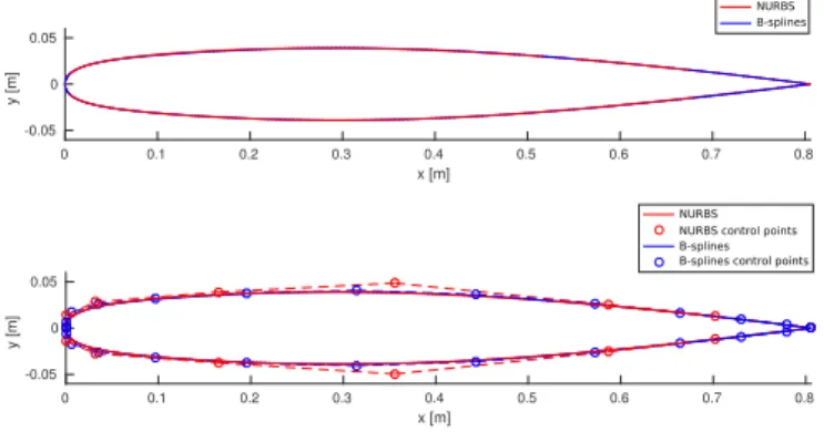
The M6 wing described using 26 B-spline control points and 16 NURBS control points are presented in Fig. 3. The comparison of one section is shown in Fig. 4.

Fig. 3 ONERA M6 wing with 26 B-spline (left) and 16 NURBS control points (right).

0 0.1 0.2 0.3 0.4 0.5 0.6 0.7 0.8 x [m] -0.05 0 0.05 y [m] NURBS B-splines 0 0.1 0.2 0.3 0.4 0.5 0.6 0.7 0.8 x [m] -0.05 0 0.05 y [m] NURBS NURBS control points B-splines B-splines control points

Fig. 4 Comparison of ONERA M6 wing root section using 26 B-spline and 16 NURBS control

points. Upper: shape of section. Lower: shape of section, control points and optimised weights. The results clearly demonstrated that by using NURBS, the number of control points required to describe the M6 wing with a given surface and curvature fidelity is significantly reduced.

5 Drag minimisation of the M6 wing

5.1 In-house solver: STAMPS

The in-house solver STAMPS [32, 29] (Source-Transformation Adjoint Multi-physics Solver) is used to perform flow analysis and provide the sensitivity of the objective function w.r.t. surface mesh node positions,∂J/∂xV. STAMPS is a

com-pressible flow solver using a vertex-centred Finite Volume Method (FVM). A dis-crete adjoint solver which is derived using the AD tool Tapenade is also included in STAMPS to provide sensitivities [9].

5.2 Case set up

The optimisation of the ONERA M6 wing in the transonic regime and inviscid flow are performed. Some set up information are listed as following:

• Mesh: tetrahedron, 135204 nodes.

• Flow conditions:Ma=0.84, Angle of attack (AoA)=3.06 ,T•=300K,p•=

101325Pa.

• Mesh deformation method: inverse distance weighting (IDW) [33].

• Control points at the leading and trailing edge are frozen to fix the AoA. Other control points can move vertically and along the chordwise direction. Weights of free control points can also change.

• Cost function: drag with lift constraints, defined as:

J=D+c⇤(L L⇤₎2_{, (15)}

whereDis the drag force,cis the penalty coefficient chosen as 0.0001,Lis lift force, andL⇤_{is the initial lift, which is 11104.21Nhere.}

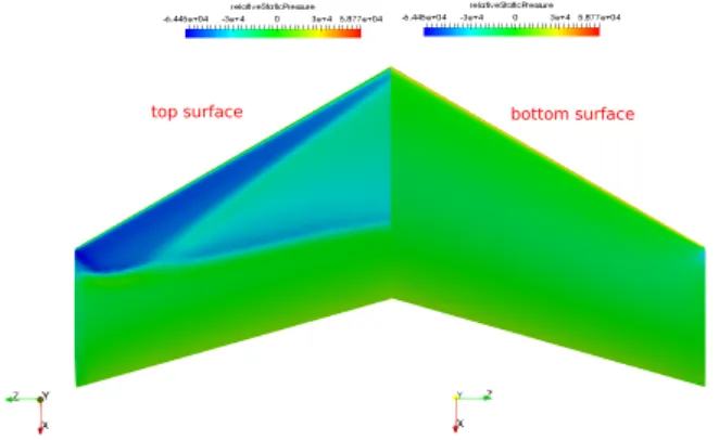
The pressure contours of the baseline geometry are shown in Fig. 5. As you can see, the typical ‘lambda’ shock on the top surface is very clear.

top surface bottom surface

Fig. 5 Baseline geometry pressure contours on top and bottom surface beformation optimisation.

5.3 Optimisation results

To investigate the effect of parametrisation on optimisation results, the M6 wing described using 26 B-splines and 16 NURBS control points for each section are used in the optimisation. The steepest descent method with Armijo line search is utilised as the optimiser [34].

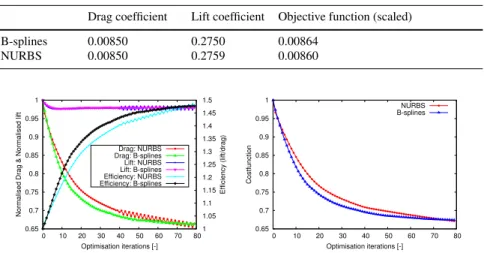
The comparison of drag, lift, efficiency (lift/drag ratio) and objective function during the optimisation are shown in Fig. 6. In both cases, the drag values are re-duced by over 30%. In the NURBS case, the optimised wing loses 1.64% of lift, which is slightly better than of B-spline case (1.98%). The loss of some lift is as ex-pected, because the penalty part in the objective function is not very strict such that more drag reduction can be achieved. Exact values of final drag and lift are listed in Table 1. Note that the NURBS case optimisation has been stopped at the same num-ber of iterations as the B-spline case, however the gradient values of the NURBS case are still much larger and further improvement with more design iterations can be expected.

Table 1 Final drag and lift coefficients

Drag coefficient Lift coefficient Objective function (scaled)

B-splines 0.00850 0.2750 0.00864 NURBS 0.00850 0.2759 0.00860 0.65 0.7 0.75 0.8 0.85 0.9 0.95 1 0 10 20 30 40 50 60 70 80 1 1.05 1.1 1.15 1.2 1.25 1.3 1.35 1.4 1.45 1.5

Normalised Drag & Normalised lift

Efficiency (lift/drag) Optimisation iterations [-] Drag: NURBS Drag: B-splines Lift: NURBS Lift: B-splines Efficiency: NURBS Efficiency: B-splines 0.65 0.7 0.75 0.8 0.85 0.9 0.95 1 0 10 20 30 40 50 60 70 80 Costfunction Optimisation iterations [-] NURBS B-splines

Fig. 6Left: The comparison of normalised drag, lift and efficiency (lift/drag ratio). Right: The

comparison of cost function.

B-splines NURBS

The comparison of pressure contours on upper surface after optimisation is pre-sented in Fig. 7, which clearly indicates that in both cases the shocks on the upper surface are reduced significantly. This is also well illustrated in Fig. 8 where the pressure coefficients on both upper and lower surface at different spanwise posi-tions are given.

-0.04 -0.03 -0.02 -0.01 0 0.01 0.02 0.03 0.04 0.1 0.2 0.3 0.4 0.5 0.6 0.7 0.8 0.9 y [m] x [m] Original NURBS B-splines

(a) 19.9% span: section shape

-1 -0.8 -0.6 -0.4 -0.2 0 0.2 0.4 0.6 0.8 1 0.1 0.2 0.3 0.4 0.5 0.6 0.7 0.8 0.9 -Cp [-] x [m] Original NURBS B-splines (b) 19.9% span: Cp -0.04 -0.03 -0.02 -0.01 0 0.01 0.02 0.03 0.04 0.3 0.4 0.5 0.6 0.7 0.8 0.9 1 y [m] x [m] Original NURBS B-splines

(c) 43.9% span: section shape

-1 -0.8 -0.6 -0.4 -0.2 0 0.2 0.4 0.6 0.8 1 1.2 0.3 0.4 0.5 0.6 0.7 0.8 0.9 1 -Cp [-] x [m] Original NURBS B-splines (d) 43.9% span: Cp -0.03 -0.02 -0.01 0 0.01 0.02 0.03 0.4 0.5 0.6 0.7 0.8 0.9 1 1.1 y [m] x [m] Original NURBS B-splines

(e) 64.8% span: section shape

-1 -0.8 -0.6 -0.4 -0.2 0 0.2 0.4 0.6 0.8 1 1.2 0.4 0.5 0.6 0.7 0.8 0.9 1 1.1 -Cp [-] x [m] Original NURBS B-splines (f) 64.8% span: Cp

Fig. 8 Comparison of cross section and pressure coefficient at different span-wise position

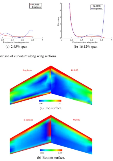
The comparison of wing profiles at different spanwise positions are given in Fig. 8. One can see that the optimised shape of in the B-splines case has a large curvature variation near the trailing edge. A clearer comparison of curvature is presented in Figs. 9 and 10, which show the curvature of the two wing sections.

and the mean curvature [35] of optimised surfaces, respectively. These figures clearly demonstrate that the optimisation using a NURBS parametrisation produces a smoother shape. The possible reason is that, when fewer control points are used, the possibility of producing noisy surface is reduced. As a consequence, the aero-dynamic performance is better, since in the transonic flow the aeroaero-dynamic per-formance is very sensitive to the shape of geometry. It is expected that when fully converged, the NURBS parametrisation will produce a lower drag since we have a much smoother variation of curvature. The smoother curvature variation will be more important in viscous flow, as strong changes in curvature will lead to rapid pressure changes which will adversely affect the boundary layer.

0 0.2 0.4 0.6 0.8 1

Position on the wing section 0 1 2 3 4 5 Curvature NURBS B-splines (a) 2.45% span 0 0.2 0.4 0.6 0.8 1

Position on the wing section 0 1 2 3 4 5 Curvature NURBS B-splines (b) 16.12% span

Fig. 9 Comparison of curvature along wing sections.

B-splines NURBS

(a) Top surface.

B-splines NURBS

(b) Bottom surface.

6 Conclusions

In this paper, NURBS have been demonstrated as an appropriate parametrisation method for wing shape optimisation. NURBS associate a weight with each control point additional freedom in controlling shapes, and have hence been shown to be capable to represent shapes accurately with fewer control points. This helps to pro-duce surface with smaller curvature variation. The optimisation results of ONERA M6 wing with both B-splines and NURBS parametrisation in transonic inviscid flow based on adjoint method have been presented. It has been shown that the optimisa-tion using a NURBS-based wing parametrisaoptimisa-tion has a smoother shape with smaller variation of curvature, which is beneficial for aerodynamic performance. This can be important in the design of turbo-machinery blades or transonic wings.

Finally, the effectiveness of CAD-based optimisation coupling the lightweight NSPCC approach with adjoint method has also been demonstrated.

Acknowledgements The first author would like to thank the China Scholarship Council

(No. 201306230097) and Queen Mary University of London for funding this research. The second author acknowledges the support from the IODA project (http://ioda.sems.qmul.ac.uk), funded by the European Union HORIZON 2020 Framework Programme for Research and Innovation under Grant Agreement No. 642959.

References

1. W. Squire and G. Trapp. Using complex variables to estimate derivatives of real functions.

SIAM-Review, 10(1):110–112, 1998.

2. A. Griewank and A. Walther.Evaluating Derivatives: Principles and Techniques of

Algorith-mic Differentiation. SIAM, Philadelphia, PA, second edition edition, 2008.

3. U. Naumann. The art of differentiating computer programs: an introduction to algorithmic

differentiation. SIAM, 2011.

4. O. Pironneau. On optimum design in fluid mechanics. Journal of Fluid Mechanics, 64:97– 110, 1974.

5. A. Jameson. Aerodynamic design via control theory.Journal of Scientific Computing, 3:233– 260, 1988.

6. A. Jameson. Optimum aerodynamic design using CFD and control theory. AIAA paper, 1729:124–131, 1995.

7. M. B. Giles, M. C. Duta, J.-D M¨uller, and N. A. Pierce. Algorithm developments for discrete adjoint methods.AIAA Journal, 41(2):198–205, 2003.

8. D. Jones, F. Christakopoulos, and J.-D. M¨uller. Preparation and assembly of adjoint CFD codes.Computers and Fluids, 46(1):282–286, 2011.

9. F. Christakopoulos, D. Jones, and J.-D. M¨uller. Pseudo-timestepping and validation for auto-matic differentiation derived code.Computers and Fluids, 46(1):174–179, 2011.

10. S. Jakobsson and O. Amoignon. Mesh deformation using radial basis functions for gradient-based aerodynamic shape optimization.Computers and Fluids, 36(6):1119 – 1136, 2007. 11. J.A. Samareh. Aerodynamic shape optimization based on free-form deformation.AIAA, paper

4630:1–13, 2004. DOI:10.2514/6.2004-4630.

12. A. Jameson and A. Vassberg. Studies of alternative numerical optimization methods applied to the brachistochrone problem.Computational Fluid Dynamics Journal, 9(3), 2000.

13. Stephan Schmidt, Caslav Ilic, Nicolas Gauger, and Volker Schulz. Shape gradients and their smoothness for practical aerodynamic design optimization. DFG SFB 1253 Preprint-Number SPP1253-10-03 http://, Universit¨at Erlangen, April 2008.

14. A. Jaworski and J.-D. M¨uller. Toward modular multigrid design optimisation. In C. Bischof and J. Utke, editors,Lecture Notes in Computational Science and Engineering, volume 64, pages 281–291, ”New York, NY, USA”, 2008. Springer.

15. T.T. Robinson, C.G. Armstrong, H.S. Chua, C. Othmer, and T. Grahs. Sensitivity-based opti-mization of parameterised CAD geometries. In8th World Congress on Structural and

Multi-disciplinary Optimisation, Lisbon, 2009.

16. S. Auriemma, M. Banovic, O. Mykhaskiv, H. Legrand, J.D. M¨uller, and A. Walther. Opti-misation of a U-bend using CAD-based adjoint method with differentiated cad kernel. In

ECCOMAS Congress, 2016.

17. S. Xu, W. Jahn, and J.-D. M¨uller. CAD-based shape optimisation with CFD using a discrete adjoint.International Journal for Numerical Methods in Fluids, 74(3):153–168, 2014. 18. X. Zhang, Y. Wang, M. Gugala, and J.-D. M¨uller. Geometric continuity constraints for

adja-cent NURBS patches in shape optimisation. InECCOMAS Congress 2016, volume 2, 2016. 19. R. Jesudasan, X. Zhang, M. Gugala, and J.D. Mueller. CAD-free vs CAD-based

parametrisa-tion method in adjoint-based aerodynamic shape optimizaparametrisa-tion. InECCOMAS Congress 2016, 2016.

20. S. Xu, D. Radford, M. Meyer, and J.-D. M¨uller. CAD-based adjoint shape optimisation of a one-stage turbine with geometric constraints. ASME Turbo Expo 2015, June 2015. GT2015-42237.

21. L. Hasco¨et and V. Pascual. Tapenade 2.1 user’s guide. Technical Report 0300, INRIA, 2004. 22. L. Piegl and W. Tiller. The NURBS Book. 2nd, 1997.

23. L. Hasco¨et and V. Pascual. The Tapenade Automatic Differentiation tool: Principles, Model, and Specification.ACM Transactions On Mathematical Software, 39(3), 2013.

24. Simon Painchaud-Ouellet, Christophe Tribes, Jean-Yves Tr´epanier, and Dominique Pelletier. Airfoil Shape Optimization Using a Nonuniform Rational B-Splines Parametrization Under Thickness Constraint.AIAA Journal, 44(10):2170–2178, 2006.

25. M. J. Pratt. Introduction to ISO 10303 - the STEP Standard for Product Data Exchange.

Journal of Computing and Information Science in Engineering, 1(1):102, 2001.

26. V Schmitt and F Charpin. Pressure distributions on the onera-m6-wing at transonic mach numbers.Experimental data base for computer program assessment, 4, 1979.

27. J. L´epine, F. Guibault, J.-Y. Tr´epanier, and F P´epin. Optimized nonuniform rational B-spline geometrical representation for aerodynamic design of wings. AIAA journal, 39(11):2033– 2041, 2001.

28. M. Gugala, S. Xu, and J-D. Mueller. Node-based vs CAD-based Approach in CFD Adjoint-based Shape Optimisation. International Conference on Engineering and Applied Sciences Optimization, Kos, Greece, 2014.

29. M. Gugala. Output-based mesh adaptation using geometric multi-grid for error estimation. PhD thesis, Queen Mary University of London, October 2017.

30. J. Nocedal. Updating quasi-newton matrices with limited storage.Mathematics of computa-tion, 35(151):773–782, 1980.

31. D. Liu and J. Nocedal. On the limited memory bfgs method for large scale optimization.

Mathematical programming, 45(1):503–528, 1989.

32. J.-D. M¨uller, M. Gugala, S. Xu, J. H¨uchelheim, P. Mohanamuraly, and O. R. Imam-Lawal. In-troducing STAMPS: an open-source discrete adjoint cfd solver usingg source-transformation ad. In11th ASMO UK/ISSMO/NOED2016: International Conference on Nuemerical

Optimi-sation Methods for Enggineering Design, 2016.

33. J.A.S Witteveen and H. Bijl. Explicit mesh deformation using inverse distance weighting interpolation. In19th AIAA Computational Fluid Dynamics, page 3996. 2009.

34. M. Bartholomew-Biggs. Nonlinear optimization with engineering applications, volume 19. Springer, 2008.

35. M Spivak. A comprehensive introduction to differential geometry, houston, tx: Publish or perish, 1999.