Volume 19
Article 1
2019
Environmental Degradation and Economics
Growth: Testing the Environmental Kuznets Curve
Hypothesis (EKC) in Six ASEAN Countries
Zhen Yang (Rex) Chng
Minnesota State University, MankatoFollow this and additional works at:
https://cornerstone.lib.mnsu.edu/jur
Part of the
Development Studies Commons
,
Economics Commons
, and the
Environmental
Studies Commons
This Article is brought to you for free and open access by the Undergraduate Research Center at Cornerstone: A Collection of Scholarly and Creative Works for Minnesota State University, Mankato. It has been accepted for inclusion in Journal of Undergraduate Research at Minnesota State University, Mankato by an authorized editor of Cornerstone: A Collection of Scholarly and Creative Works for Minnesota State University, Mankato.
Recommended Citation
Chng, Zhen Yang (Rex) (2019) "Environmental Degradation and Economics Growth: Testing the Environmental Kuznets Curve Hypothesis (EKC) in Six ASEAN Countries,"Journal of Undergraduate Research at Minnesota State University, Mankato: Vol. 19 , Article 1.
Undergraduate Research Center.
I/We certify have followed the accepted standards of scientific, creative, and academic honesty and
ethics.
I understand that my article submission will be blind-reviewed by faculty reviewers who will recommend
acceptance for publication; acceptance with revisions; or reject for publication.
I understand that as author, I retain the right to present any part of the research in any form in other
publications.
The JUR has the right to reproduce and reprint published submissions for instructional or promotional
purposes.
For complete details, see
Journal of Undergraduate Research at Minnesota State University, Mankato policies
page.
Mentor Agreement:
I have reviewed the submission, and I support its inclusion in the JUR (The Journal of Undergraduate
Research at Minnesota State University, Mankato). I understand that I will be acknowledged as the
faculty mentor for the student author(s). To the best of my knowledge, the student has followed the
accepted standards of scientific, creative, and academic honesty and ethics.
ENVIRONMENTAL DEGRADATION AND ECONOMIC GROWTH: TESTING
ENVIRONMENTAL KUZNETS CURVE HYPOTHESIS IN SIX ASEAN COUNTRIES
Zhen Yang (Rex) Chng, Minnesota State University, Mankato, USA ABSTRACT
Environmental issues have been widely reported in recent years. From climate change to plastic waste, environmental quality is deteriorating at an unprecedented speed in human history. Environmental degradation is believed to have tied to the different stages of a country’s economic growth, as the Environmental Kuznets Curve (EKC) hypothesis suggested. Despite the proliferation of research about the EKC hypothesis, no consensus has been reached in the field regarding the validation of the hypothesis. This paper employs time-series methods to empirically investigates the impacts of economic growth, trade openness, energy consumption, and foreign direct investment on environmental degradation in six selected ASEAN countries, from the period between 1971 to 2013, to examine the validity of the EKC hypothesis. First, Augmented Dickey-Fuller (ADF) and Phillips-Perron (PP) tests were applied to test the stationarity of selected variables, Johansen Cointegration test and ARDL bound testing for cointegration test, ARDL models were constructed to find the potential long- and short-run relationships. The results showed the presence of EKC in Singapore, Thailand, and Vietnam, and no evidence of EKC was found in Malaysia, Philippines, and Indonesia.
Keywords: Environmental Kuznets Curve, ASEAN, Environmental Degradation, Economic
Growth, CO2 Emissions, Energy Consumption, Trade, Foreign Direct Investment
I. INTRODUCTION
Environmental issues have been widely reported in recent years. From climate change to plastic waste to deforestation, environmental quality is deteriorating at an unprecedented speed in human history, as many countries put economic growth as their top priority at the expense of the environment. Global warming has been reported to be posing severe threats to the future of humanity. The primary cause of this global phenomenon is contributed by the emissions of greenhouse gases, with carbon dioxide (CO2) emissions sharing the largest portion. There has been a 60 percent increase in global CO2
emissions from 1990 to 2013, which causes a rise of 0.8 degrees Celsius in mean global temperature when combining with other greenhouse gases (Khokhar, 2017). A similar report from Intergovernmental Panel on Climate Change (2014) explained that 78 percent of CO2 emissions in the shared
greenhouses gases comes from the fossil fuel combustion from 1970 to 2010. Environmentalists have repeatedly warned that the consequences of the rising temperature will be a disaster if the levels of CO2 and other greenhouse gas emissions are left uncapped and continue to rise.
As global warming becomes a dire issue, a great number of researches in the past decades has been focused on examining the link between CO2 emissions levels and the pace of environmental
degradation. By using CO2 emissions level as a proxy of environment, some studies revealed that the
deterioration of environment is associated with the economic growth of a country (Azomahou et. Al, 2006; Mladenović et al, 2016). To dive deeper into the complexity of the subject, some researchers also incorporated exogenous factors such as trade openness, foreign direct investment, energy usage, and population growth in their study along with growth rate, in searching for a better understanding of this problem and for environmental policies implications. Regardless of the growing research in the realm, the conclusion of economic growth affectingenvironmental degradation due to the CO2 emissions
release from economic activities remains an enigma, as each study applied a slightly different strategy or method while researching this topic.
This paper, therefore, intends to investigate the relationship between environmental degradation and economic growth with the presence of energy consumption, trade openness, and foreign direct investment in six selected Southeast Asia countries.
(A) ENVIRONMENTAL KUZNETS CURVE (EKC) HYPOTHESIS
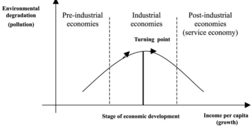
Environmental degradation is believed to have tied to the stages of economic growth. Environmental experts argued that pursuing solely on economic growth will put the environment in jeopardy. An early piece of research by Grossman and Krueger (1991,1995) investigated the nexus of environmental degradation and economic growth. They noticed that there exists an inverted U-shaped curve identical to the Kuznets curve, and named it the Environmental Kuznets Curve (EKC). Kuznets (1955) proposed that economic inequality will first increase and then decrease after reaching the highest point where the economy continues to develop throughout the process, showing an inverted U-shaped curve among the relationship of economic inequality and income per capita. Analogously, the EKC hypothesis suggested that the environment will initially deteriorate as an economy takes off. However, the environment quality of a country will start improving once the income level hit a turning point. In other words, the hypothesis implies there is a self-fixing mechanism between environmental degradation and economic growth, which the best solution to solving a country’s environmental deterioration is its economic growth.
Equally important, some studies also suggested the relationship between environmental quality and growth is an N-shaped or inverted N-shaped curve, instead of an inverted U-shaped curve (Churchil, Inekwe, Ivanovski, & Smyth, 2018), or more generally, the shape of curves may vary as each country develops in a different pace (Hwa, Li, Khan, & Hong, 2016). The inverted U-shaped curve which EKC proposed is illustrated in figure 1
Figure 1. Environmental Kuznets Curve Sources: Panayotou (1993)
Since the 1990s, a proliferation of empirical studies has attempted to examine the relationship between economic growth and environmental quality in different countries under the EKC hypothesis. Although many studies have repeatedly examined the EKC hypothesis, validation of the hypothesis remains inconclusive because the results vary from one study to another. This is mainly due to the selection of variables, countries, and timespan, or more specifically, the specification of the econometrics model constructed in each study (Ahmad, at al., 2017; Harbaugh, Levinson, and Wilson, 2002). Nevertheless, the EKC hypothesis provided a basic framework to how environmental degradation related to economic growth. As a reason, this paper intends to investigate the impacts of economic growth, foreign direct investment (FDI), trade liberalization, and energy consumption on the environmental degradation in six selected countries of the Association Southeast Asia Nations (ASEAN), from the period of 1971 to 2013, to examine the validity of the EKC hypothesis.
(B) ASEAN CONTEXT
With more than 600 million population and plenty of natural resources, Southeast Asia is regarded as one of the fast-growing regions in the world for the past couple of decades. The regional economic bloc-ASEAN was first established in 1967, with the notions of promoting economic collaboration, maintaining regional peace and stability, and enhancing cultural exchange among its member states. According to Wood (2017), published on World Economic Forum, “If ASEAN were a country, it would be the seventh-largest economy in the world, with a combined GDP of $2.6 trillion in 2014. By 2050 it is projected to
rank as the fourth-largest economy”. As a region now experiencing a high economic growth, ASEAN nations are in dire dilemma of choosing between sacrificing the environment by prioritizing the robust growth or protecting the environment by forgoing the economic boom.
An extensive amount of literature about the EKC hypothesis in the context of ASEAN have been predominantly focusing on the five founding members (Singapore, Malaysia, Indonesia, Thailand, & Philippines) of the organization, the rest of the member states (Vietnam, Laos, Myanmar, Cambodia, and Brunei) are often being excluded mainly due to the incompleteness of the data available for research. Because of this, painting a full picture of the environmental condition vis-à-vis to the growth rate in ASEAN can be difficult without including most of its member states. For this reason, the goal of this paper is to study the effects of growth, FDI, trade, energy usage with respect to the environmental quality under the assumption of the EKC hypothesis, to understand which variables are significant to the environmental degradation in the selected ASEAN nations.
II. LITERATURE REVIEW
Vast amounts of studies have examined the impacts of economic growth, FDI, trade, and energy usage on environmental degradation, which are represented by CO2 emission in many studies, and claimed
that there is indeed an inverted U-shaped relationship as the EKC hypothesis suggested. On the contrary, some researchers questioned the validity of the EKC hypothesis, as their studies found only a little empirical evidence to support the inverted U-shaped relationship between economic growth and environmental degradation.
Narayan and Narayan (2010) studied the EKC hypothesis on 43 developing countries based on the income elasticity in short- and long-run, which they found that 35 percent of the selected countries showed a reduction in CO2 emission level as income increased, and the emission was lower in the
long-run as opposed to in the short-long-run as suggested by EKC hypothesis. The research of Apergis and Ozturk (2015) in Vietnam from 1990 to 2011, supported the existence of an inverted-U shaped relationship between CO2 emission and income per capita. In their panel study regarding the linkage of
economic growth, financial and instructional development on environmental degradation, Tamazian and Rao (2010) found that economic development did lower the environmental quality, but the degradation began to reduce when both financial and institutional variables were taken into account, which confirmed that EKC hypothesis is valid.
Conversely, Adu and Denkyirah (2017) incorporated CO2 emission and combustible renewable waste
as their indicators of the environment when examining the EKC hypothesis. The result concluded that economic growth negatively impacts in West Africa in the short-run as the two pollutants increased along the economy, but no significant decrease was found in both pollutant indicators in the long-run, meaning that EKC hypothesis is illegitimate. Harbaugh, Levinson, and Wilson (2002) used three types of air pollutants (SO2, smoke, and TSP) as the environmental variable and national income level to test
the robustness of the EKC hypothesis, they argued that there were no significant amounts of empirical evidence available to justify the EKC hypothesis because both pollutions and growth are sensitive to sample selections and model specifications.
In the realm of energy consumption, Beak and Kim (2013) studied the environment and economic growth by looking at the level of energy consumption, as well as the fossil fuels and nuclear energy in electricity production in Korea. Their study showed that the environment started to degrade when income per capita increased, the degradation has improved since the last couple of decades while the economy continues to grow, which subsequently proved the existence of EKC hypothesis in this case. Furthermore, Gokmenoglu and Taspinar (2016) tested the EKC hypothesis in Turkey from 1974 to 2010 by incorporating CO2 emission, energy consumption, FDI, and growth rate. The results indicated that
the air pollution decreases when GDP increases in the long-run, whereas a reverse relationship between the two variables is true in the short-run, thus concluded that EKC hypothesis is valid. Ahmad et al. (2017), on the other hand, applied Autoregressive Distributed Lag (ARDL) method to test the EKC hypothesis in Croatia across a timespan of 20 years. They used CO2 emission as the
dependent variable for the environment to find the relationship with economic growth, and their result showed the hypothesis only holds in the long-run and with no conclusive evidence available in the short-run. Similarly, Le and Quah (2018) explored the nexus of CO2 emission, energy consumption and
economic growth in fourteen selected countries in Asia-Pacific. Their study discovered that the EKC hypothesis holds in high-income countries, whereas the opposite of the hypothesis was true for low-
and middle-income countries, which showed that economic growth reduced the CO2 emission rather
than increased it in the short-run. Lastly, Pau, Yu, and Yang (2011) researched the relationship between environment, growth, and energy consumption in Russia from 1990 to 2007 by using CO2 emission
level as an environmental indicator. The results showed that economic growth has an insignificant impact on CO2 emission, which rejected the EKC hypothesis. They also stated that enforcing effective
economic and energy policies could reduce the CO2 emission level without suppressing economic
development.
Several studies have found that EKC hypothesis is valid when incorporated FDI and/or trade into the model. Twerefou, Danson-Mensah, and Bokpin (2017) investigated the impacts of globalization on the environment quality by using growth, foreign direct investment (FDI), and trade as their indicators. They validated the EKC hypothesis in their study as there exists a positive relationship between the environment and economic growth, which portended that the expansion of globalization will inevitably cause the environmental quality to deteriorate in Sub-Saharan Africa countries. Additionally, Hitam and Borhan (2012) examined the pollution and FDI in Malaysia for the period of 1965 to 2010 and stated that environmental degradation was linked to the level of FDI, which higher level of FDI will have harmful effects on the environment, therefore concluded that the EKC hypothesis is true. The research of Hwa, Li, Khan, and Hong (2016) concluded that the EKC hypothesis exists in the five founding members of ASEAN when including FDI and trade as controlled variables. Their results, however, suggested that the relationship between CO2 emission and economic growth in both short- and long-run has shown an
inverted-S shaped, rather than the orthodox inverted U-shaped.
In contrast, Zhu, Duan, Guo, and Yu (2016) utilized a panel quantile regression method to search for the effects of growth, FDI, and energy consumption on CO2 emission level in five selected ASEAN
nations. Their study revealed that the effects of each variable on CO2 emission level were
heterogeneous in different quantiles, which indicated that there were no consistent results able to validate the EKC hypothesis holds for all five of the ASEAN nations. In a time-series data analysis of Pakistan, Ahmed and Long (2012) deployed CO2 emission level as the environment variable and
investigated its relationship with growth, energy consumption, trade, and population density. Their study found that EKC hypothesis holds in the long-run because all explanatory variables were statistically significant to the CO2 emission level, but no relationship was found in the short-run, which failed to
prove the existence of EKC hypothesis.
To contribute to the existing EKC hypothesis literatures, this paper attempts to research the environment-income nexus with the presence of energy consumption, foreign direct investment, and trade openness in selected ASEAN countries, from 1971 to 2013, by applying time-series econometric tools.
III. THE EMPIRICAL FRAMEWORK & DATA
(A) EMPIRICAL MODEL
This paper employs time-series methods to examine the environment-income-energy-trade-FDI nexus in selected ASEAN countries. Following the empirical research in environmental economics, a time-series empirical model of which constructed to evaluate EKC hypothesis in each ASEAN country is expressed as:
(𝑙𝑛𝐶𝑂2)𝑡 = β0+ β1(𝑙𝑛𝐺𝐷𝑃𝑝𝑐)𝑡+ β2(𝑙𝑛𝐺𝐷𝑃𝑝𝑐) 2
𝑡+ β3 (𝑙𝑛𝐸𝐶)𝑡+ β4 (𝑙𝑛𝐹𝐷𝐼)𝑡+ β5 (𝑙𝑛𝑇𝑅)𝑡+ 𝑡 (1) where the 𝐶𝑂2 is the carbon dioxide emission level in period 𝑡, measures by metric tons per capita. It also serves as a proxy for environmental degradation. All dependent and independent variables are transformed into logarithm form to interpret the elasticity of the parameters. 𝐺𝐷𝑃𝑝𝑐 represents income per capita, measures in constant 2010 US dollar. 𝐸𝐶 is energy consumption measured in kg of oil equivalent per capita per capita. Moreover, 𝐹𝐷𝐼 is the net inflow of foreign direct investment calculated
in constant 2010 US dollar, whereas 𝑇𝑅 represents trade level measuring as the sum of export and import to GDP ratio in constant 2010 US dollar. Lastly, β0and 𝑡 are the constant term and standard error term.
GDP per capita (𝐺𝐷𝑃𝑝𝑐), energy consumption (𝐸𝐶), net inflow of foreign direct investment (𝐹𝐷𝐼), and trade openness (𝑇𝑅) are all expected to have a positive relationship with the level of CO2 emission
level (𝐶𝑂2), whereas the square of GDP per capita (𝐺𝐷𝑃𝑝𝑐2) is presumed to be negatively related to CO2
emission level. According to Twerefou, Danson-Mensah, and Bokpin (2017), three potential outcomes may occur when regress the empirical model:
(1) When β1> 0 and β2= 0, there exists a linear relationship between CO2 emission and
economic growth, suggesting that an increasing growth rate leads to an increasing in CO2 emission.
(2) When β1< 0 and β2> 0, there exists a U-shaped relationship between CO2 emission and
economic growth.
(3) When β1> 0 and β2< 0, there exists an inverted U-shaped curve and validate EKC hypothesis. Moreover, the estimation of turning point in EKC hypothesis can be expressed as followed 𝐺𝐷𝑃𝑝𝑐∗ =
−(β1 /2β2). As the income per capita (GDPpc) is represented in logarithm form, the peak of GDPpc∗ can be calculated by using the formula proposed by de Bruyn and Opschoor (1998), which specified as 𝐺𝐷𝑃𝑝𝑐∗ = 𝑒−(β1/2β2) .
(B) UNIT-ROOT TEST & COINTEGRATION TEST
Two different unit-root tests, augmented Dickey-Fuller (ADF) test and Philips-Perron (PP) test, are used to examine if all variables have presence of unit root. The null hypothesis of both tests is stated as variable has unit-root, which means the variable is non-stationary. If the parameters of the variables are not statistically significant, then the null hypothesis can be rejected. All variables are expected to be non-stationary at level, 𝐼(1) process, and stationary after converting to first difference, 𝐼(0) process. After performing both stationary tests, Johansen cointegration test is utilized to check whether there exhibit combinations of cointegration among the chosen variables. The null hypothesis of Johansen cointegration states that there is no cointegration among selected variables in the long-run. If null hypothesis is rejected, then the existence of long-run relationship among the variables can be established.
(C) AUTOREGRSSIVE DISTRIBUTION LAG (ARDL) MODEL
To further the test of cointegration, Autoregressive Distribution Lag (ARDL) method is applied for this regard. ARDL method developed by Pesaran et al. (2001) is particularly useful in testing the cointegration among variables.
Several studies (Saboori, Sulaiman, & Mohd, 2012; Saboori & Sulaiman, 2013; Gokmenoglu & Taspinar, 2016; Ahmad et al., 2017) employed ARDL method to test cointegration mainly because of three major advantages. Firstly, the conventional cointegration techniques such as Johansen cointegration test and Engle-Granger cointegration test require all independent variables to be at a same level of time-series process, for example, they must all be at 𝐼(1) process. ARDL method, on the other hand, does not require all variables to have the same process, it can be applied whether the variables are 𝐼(1), 𝐼(0), or a mixture of both, but no variables can be in 𝐼(2). Second reason is that the impacts of independent variables on dependent variable in both long- and short-run can be assessed simultaneously, which makes distinguishing long- and short-run effects relatively effortless. Lastly, Pesaran and Shin (1998) found that consistency in the OLS estimators of the short-run parameters and the ARDL based estimators of the long-run coefficients in small sample sizes.
𝑙𝑛(𝐶𝑂2)𝑡=0+ ∑1k 𝑙𝑛(𝐶𝑂2)𝑡−𝑘 𝑛 𝑘=1 + ∑2k 𝑙𝑛(𝐺𝐷𝑃𝑝𝑐)𝑡−𝑘 𝑛 𝑘=0 + ∑3k 𝑙𝑛 (𝐺𝐷𝑃𝑝𝑐) 2 𝑡−𝑘 𝑛 𝑘=0 + ∑4k 𝑙𝑛(𝐸𝐶)𝑡−𝑘 𝑛 𝑘=0 + ∑5k 𝑙𝑛(𝐹𝐷𝐼)𝑡−𝑘 𝑛 𝑘=0 + ∑6k 𝑙𝑛(𝑇𝑅)𝑡−𝑘 𝑛 𝑘=0 +1𝑙𝑛(𝐶𝑂2)𝑡−1 +2𝑙𝑛(𝐺𝐷𝑃𝑝𝑐)𝑡−1+3𝑙𝑛 (𝐺𝐷𝑃𝑝𝑐) 2 𝑡−1+4 𝑙𝑛(𝐸𝐶)𝑡−1+5 𝑙𝑛(𝐹𝐷𝐼)𝑡−1+6𝑙𝑛(𝑇𝑅)𝑡−1 + 𝑡 (2) where in equation (2) 1k, 2k, 3k, 4k, 5k, and 6k represent the short-run error-correction dynamics, 1, 2, 3, 4, 5, and 6 show the long-run dynamics, 0 is constant term, and 𝑡 is white noise error term. The null hypothesis of ARDL bound testing for cointegration is 𝐻0:1=2=3=4=5= 0, which suggest no cointegration, and the alternative hypothesis is 𝐻0:1 2 3 4 5 0. Pesaran et al. (2001) introduced two set of critical values for which known as lower bound and upper bound. The former is for 𝐼(0) variables, whereas the latter considers 𝐼(1) variables. When the computed F-statistics is smaller than lower bound critical value, then null hypothesis cannot be rejected, and null hypothesis can be rejected when the F-statistics is greater than upper bound critical value. If the F-statistics fall between lower and upper bound, then the result is inconclusive.
When the F-statistics fall in the inconclusive zone, Banarjee et al. (1998) explained the long-run relationship can be established if the error-correction term is negative and significant statistically. Corroborating with Banarjee et al. (1998), Saboori and Sulaiman (2013) suggested that substituting all lagged level variables with error-correction term, and then test if the coefficients are statistically significant. After establishing the existence of long-run relationship, error-correction model (𝐸𝐶𝑀) is employed to estimate the short-run coefficients and error-correction term. Equation (3) shows the general formula of 𝐸𝐶𝑀: 𝑙𝑛(𝐶𝑂2)𝑡=0+ ∑1k 𝑙𝑛(𝐶𝑂2)𝑡−𝑘 𝑛 𝑘=1 + ∑2k 𝑙𝑛(𝐺𝐷𝑃𝑝𝑐)𝑡−𝑘 𝑛 𝑘=0 + ∑3k 𝑙𝑛 (𝐺𝐷𝑃𝑝𝑐) 2 𝑡−𝑘 𝑛 𝑘=0 + ∑4k 𝑙𝑛(𝐸𝐶)𝑡−𝑘 𝑛 𝑘=0 + ∑5k 𝑙𝑛(𝐹𝐷𝐼)𝑡−𝑘 𝑛 𝑘=0 + ∑6k 𝑙𝑛(𝑇𝑅)𝑡−𝑘 𝑛 𝑘=0 +∗ 𝐸𝐶𝑇𝑡−1+ 𝑡 (3) where ∗ 𝐸𝐶𝑇𝑡−1 is the error-correction term representing the speed of adjustment in which how fast the variables adjust to the long-run equilibrium level. In addition, diagnostic tests such as normality, serial correlation, and heteroskedasticity tests are applied in order to ensure the goodness-of-fit of the estimated models.
(D) DATA
This paper applied annual data across a timespan of 43 years, from 1971 to 2013, in the six selected ASEAN nations, which are Singapore, Malaysia, Indonesia, Thailand, Philippines, and Vietnam. All data collected are secondary data. Carbon dioxide emissions (𝐶𝑂2) and energy consumption (𝐸𝐶) are extracted from the World Development Indicator (WDI), GDP per capita (𝐺𝐷𝑃𝑝𝑐) and inward foreign direct investment (𝐹𝐷𝐼) are collected from United Nations Conference on Trade and Development (UNCTAD), and trade (𝑇𝑅) data is gathered from International Monetary Fund (IMF). Due to the severe lack of data availability in Cambodia, Myanmar, Brunei, and Lao Republic, these four countries are excluded in this analysis. Table 1 provides a summary for the definition, notation, measurement, and expected sign of all variables.
Table. 1 - Definition, notation, and expected sign of variables
Variables Types of
variables Notation Measurement Expected sign
Carbon dioxide
emissions Dependent CO2
Carbon dioxide emissions (metric
tons per capita)
No prediction
GDP per capita Independent GDP GDP per capita
(constant 2010 US$) Positive
GDP per capita squared Independent GDP2 Squared of GDP per capita (constant 2010 US$) Negative Energy consumption Independent EC
Energy use (kg of oil equivalent per capita) Positive Foreign direct investment (net inflow) Independent FDI Foreign direct investment, net inflows (constant 2010 US$) Positive Trade Independent TR (Export+Import)/GDP
(constant 2010 US$) Positive
IV. EMPIRICAL RESULTS
(A) UNIT-ROOT TEST & COINTEGRATION TEST
Two unit-root tests, augmented Dickey-Fuller test and Phillips-Perron test, were performed to examine the stationarity of all selected variables. The summary of the unit-root test results is presented in Table 2. The results obtained from ADF test and PP test highly suggested that all series have unit-root at level, which means that they are non-stationary and are 𝐼(1) process. Furthermore, the results also showed that all variables become 𝐼(0) process after converting to first difference, which indicated that they are free from unit-root and are stationary at first difference.
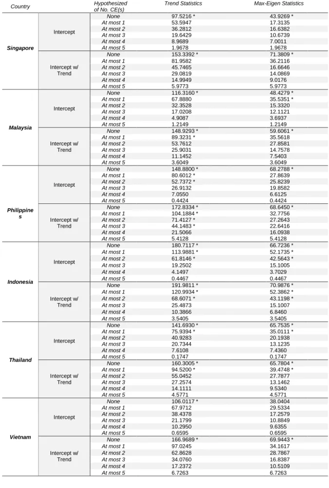
After establishing all variables were stationary at first difference, Johansen cointegration test was applied to check the cointegration among selected variables. The summary of Johansen cointegration test is illustrated in Table 3. From the table 3, the results suggest that all series are cointegrated at some combinations, which subsequently indicates that there exist long-run relationships among the variables.
Table 2 – Results of ADF Test and PP Test
Country Variables
ADF Test Statistics PP Test Statistics Trend &
Intercept
Intercept None Trend & Intercept Intercept None Singapore Level ln (CO2) -3.0984 -2.5700 -0.0789 -3.0046 -2.6088* 0.1458 ln (GDPpc) -2.5970 -1.6907 1.9701 -2.6318 -2.6412* 3.9538 ln (GDPpc)2 -2.6355 -1.2947 2.0210 -2.3481 -1.7670 3.8074 ln (EC) -1.5794 -1.9657 1.5232 -1.5152 -1.9930 1.6200 ln (FDI) -4.7529*** -1.9970 1.7609 -4.7234*** -1.3807 3.2786 ln (TR) -2.6543 -2.9819** 0.0604 -2.6113 -2.9640** 0.0766 1st difference ln (CO2) -6.3541*** -6.3675*** -6.4569*** -8.0192*** -7.7124*** -7.8511*** ln (GDPpc) -3.7410** -3.5821** -2.6969*** -3.6335** -3.4445** -2.5741** ln (GDPpc)2 -3.8677** -3.8093*** -2.7183*** -3.8154** -3.7342*** -2.7183*** ln (EC) -7.3032*** -7.1523*** -6.8599*** -7.3130*** -7.1523*** -6.8617*** ln (FDI) -6.5967*** -6.1612*** -7.8905*** -26.900*** -19.574*** -8.1649*** ln (TR) -6.9101*** -6.6297*** -6.6639*** -6.9070*** -6.6255*** -6.6590*** Malaysia Level ln (CO2) -2.1168 -0.7440 2.3785 -2.1326 -0.7440 2.5315 ln (GDPpc) -3.2337* -2.1257 3.9337 -3.2337* -2.1257 3.5453 ln (GDPpc)2 -2.7549 -1.3276 3.7403 -2.8361 -1.3276 3.7403 ln (EC) -1.9929 -0.9897 3.9731 -2.0328 -1.4455 4.6310 ln (FDI) -3.6516** -2.1682 0.7346 -3.5886** -2.0149 1.1190 ln (TR) -0.5084 -1.5958 -0.9849 -0.4409 -1.5906 -0.7388 1st difference ln (CO2) -7.7410*** -7.8174*** -6.3481*** -7.7274*** -7.7583*** -6.5236*** ln (GDPpc) -5.1887*** -5.0920*** -4.0188*** -5.1232*** -5.0104*** -3.8701*** ln (GDPpc)2 -5.3878*** -5.4036*** -4.2045*** -5.3352*** -5.3479*** -4.0919*** ln (EC) -6.7843*** -6.7102*** -4.8387*** -9.4111*** -7.0083*** -4.9210*** ln (FDI) -8.4637*** -8.5236*** -8.2981*** -8.5227*** -8.5814*** -8.3288*** ln (TR) -6.1624*** -5.6755*** -5.4797*** -6.1945*** -5.6743*** -5.5064*** Philippines Level ln (CO2) -1.5047 -0.9333 -1.0608 -1.7919 -1.2573 -1.1343 ln (GDPpc) -2.1372 -1.3042 3.7132 -2.4351 -1.3035 2.7657 ln (GDPpc)2 -1.6216 -0.6334 3.6546 -2.1007 -0.7947 2.7454 ln (EC) -2.4503 -2.5642 0.3549 -2.4470 -2.5786 0.4190 ln (FDI) -4.5333*** -3.0039** 0.6228 -4.4630** -2.3058 0.9637 ln (TR) -0.2245 -1.3247 -1.1748 -0.6311 -1.4204 -1.1186 1st difference ln (CO2) -5.6692*** -5.7114*** -5.6950*** -5.7576*** -5.7995*** -5.7859*** ln (GDPpc) -4.3716*** -4.3985*** -3.5817*** -4.4534*** -4.4640*** -3.5695*** ln (GDPpc)2 -4.4757*** -4.5333*** -3.6679*** -4.5533*** -4.6063*** -3.6799*** ln (EC) -8.9281*** -8.7972*** -8.8499*** -8.5859*** -8.4529*** -8.5051*** ln (FDI) -9.4473*** -9.3910*** -9.2234*** -13.263*** -11.629*** -10.121*** ln (TR) -5.3258*** -5.0068*** -5.0089*** -5.3675*** -5.0500*** -5.0463*** Indonesia Level ln (CO2) -3.3918* -1.5387 -1.7845* -3.2868* -1.7885 -1.7594* ln (GDPpc) -2.7305 -1.8887 2.6584 -2.7894 -1.8621 2.4170 ln (GDPpc)2 -2.1299 -1.0834 2.5126 -2.2967 -1.0927 2.4425 ln (EC) -1.2301 -1.0311 4.3041 -1.2301 -1.0769 4.5184 ln (FDI) -4.6162*** -4.6057*** -0.2197 -4.6045*** -4.5933*** -0.0326 ln (TR) -4.5067*** -3.8248*** -1.1152 -4.5306*** -3.8043*** -1.3266 1st difference ln (CO2) -5.9419*** -5.9757*** -4.9286*** -5.5454*** -5.4411*** -4.9286*** ln (GDPpc) -5.7837*** -5.7681*** -4.9960*** -5.7751*** -5.7550*** -5.0172*** ln (GDPpc)2 -5.8891*** -5.9566*** -5.1409*** -5.8802*** -5.9481*** -5.1808*** ln (EC) -6.5466*** -6.4875*** -4.6667*** -6.5832*** -6.4956*** -4.7409*** ln (FDI) -9.3430*** -9.4468*** -9.5601*** -16.9327*** -15.5857*** -15.5551*** ln (TR) -8.5685*** -8.5888*** -8.6333*** -9.5195*** -9.3022*** -9.3184*** Thailand Level ln (CO2) -1.4189 -0.8927 0.6035 -1.1017 -1.1183 0.7056 ln (GDPpc) -2.9211 -1.5876 2.2255 -2.3018 -1.5470 3.5264 ln (GDPpc)2 -2.7430 -0.9989 2.1359 -2.1910 -0.8551 3.3096 ln (EC) -2.0108 0.2807 5.5937 -2.0339 0.0647 4.2686 ln (FDI) -3.8234** -1.0755 1.4124 -3.9052** -1.3257 1.7079 ln (TR) -2.4624 -1.4036 -2.7555*** -2.5512 -1.4036 -2.8576*** 1st difference ln (CO2) -4.3909*** -4.3807*** -3.2274*** -4.3886*** -4.3780*** -3.2274*** ln (GDPpc) -4.1307** -4.0467*** -2.9767*** -4.1307** -4.0467*** -2.9483*** ln (GDPpc)2 -4.1508** -4.1797*** -3.0918*** -4.1508** -4.1797*** -2.9379*** ln (EC) -4.7380*** -4.7736*** -3.1779*** -4.8373*** -4.8691*** -3.2184*** ln (FDI) -9.0663*** -9.1804*** -8.7904*** -10.1200*** -10.2067*** -8.7904*** ln (TR) -7.1648*** -7.1418*** -6.3062*** -7.2400*** -7.1514*** -6.3120*** Vietnam Level ln (CO2) -2.3637 0.4604 -0.5859 -2.4578 0.3900 -0.6524 ln (GDPpc) -2.5052 1.0080 1.9872 -1.6121 0.8460 2.9006 ln (GDPpc)2 -1.8352 0.6112 2.6395 -1.1709 1.6529 3.7871 ln (EC) -1.6393 2.0739 2.2437 -1.6481 1.6228 2.0559 ln (FDI) -3.9011** -1.2215 -0.1613 -4.0036** -0.8458 0.3242 ln (TR) -4.2508*** -2.0378 -2.3630** -4.0722** -1.9039 -2.6193 1st difference ln (CO2) -7.6112*** -6.7186*** -6.5026*** -7.5886*** -6.7274*** -6.5593*** ln (GDPpc) -3.5466** -2.7504** -1.5808 -4.9301*** -4.2657*** -4.0204*** ln (GDPpc)2 -3.6436** -4.4402*** -3.4077*** -4.8403*** -4.2384*** -3.8387*** ln (EC) -6.8838*** -5.2200*** -4.5520*** -6.8817*** -5.4860*** -4.8696*** ln (FDI) -11.1632*** -11.1907*** -10.5451*** -10.5498*** -10.5704*** -9.8846*** ln (TR) -3.6558** -3.4027** -7.7603*** -23.0100*** -16.2871*** -7.9915***
Note: *, **, and *** represents 10%, 5%, and 1% level of significance, respectively. ADF & PP Null hypothesis: Variable has unit root.
Table 3 – Results of Johansen Cointegration Test
Country Hypothesized
of No. CE(s)
Trend Statistics Max-Eigen Statistics
Singapore Intercept None 97.5216 * 43.9269 * At most 1 53.5947 17.3135 At most 2 36.2812 16.6382 At most 3 19.6429 10.6739 At most 4 8.9689 7.0011 At most 5 1.9678 1.9678 Intercept w/ Trend None 153.3392 * 71.3809 * At most 1 81.9582 36.2116 At most 2 45.7465 16.6646 At most 3 29.0819 14.0869 At most 4 14.9949 9.0176 At most 5 5.9773 5.9773 Malaysia Intercept None 116.3160 * 48.4279 * At most 1 67.8880 35.5351 * At most 2 32.3528 15.3320 At most 3 17.0208 12.1121 At most 4 4.9087 3.6937 At most 5 1.2149 1.2149 Intercept w/ Trend None 148.9293 * 59.6061 * At most 1 89.3231 * 35.5618 At most 2 53.7612 27.8581 At most 3 25.9031 14.7578 At most 4 11.1452 7.5403 At most 5 3.6049 3.6049 Philippine s Intercept None 148.8800 * 68.2788 * At most 1 80.6012 * 27.8639 At most 2 52.7372 * 25.8239 At most 3 26.9132 19.8582 At most 4 7.0550 6.6125 At most 5 0.4424 0.4424 Intercept w/ Trend None 172.8334 * 68.6450 * At most 1 104.1884 * 32.7756 At most 2 71.4127 * 27.2643 At most 3 44.1483 * 22.6416 At most 4 21.5066 16.0938 At most 5 5.4128 5.4128 Indonesia Intercept None 180.7117 * 66.7236 * At most 1 113.9881 * 52.1735 * At most 2 61.8146 * 42.5643 * At most 3 19.2502 15.1005 At most 4 4.1497 3.7029 At most 5 0.4467 0.4467 Intercept w/ Trend None 191.9811 * 70.9876 * At most 1 120.9934 * 52.3862 * At most 2 68.6071 * 43.1198 * At most 3 25.4873 15.1007 At most 4 10.3866 6.8460 At most 5 3.5405 3.5405 Thailand Intercept None 141.6930 * 65.7535 * At most 1 75.9394 * 35.0111 * At most 2 40.9283 20.1938 At most 3 20.7344 13.1235 At most 4 7.6108 7.4360 At most 5 0.1747 0.1747 Intercept w/ Trend None 160.3005 * 65.7804 * At most 1 94.5200 * 39.4748 * At most 2 55.0452 27.7877 At most 3 27.2574 13.1462 At most 4 14.1111 9.5340 At most 5 4.5771 4.5771 Vietnam Intercept None 106.0117 * 38.0404 At most 1 67.9712 29.5334 At most 2 38.4378 17.2579 At most 3 21.1799 10.8849 At most 4 10.2950 9.6355 At most 5 0.6595 0.6595 Intercept w/ Trend None 166.9689 * 69.9443 * At most 1 97.0245 34.1617 At most 2 62.8628 28.7867 At most 3 34.0760 16.8387 At most 4 17.2372 10.5109 At most 5 6.7263 6.7263
(B) ARDL MODEL
Pesaran et al. (2001) specified that ARDL bound testing can only be applied to series that are in 𝐼(1), 𝐼(0), or the combination of both, without presence of 𝐼(2) in any of the variables. After applying ADF test and PP test to check the stationarity, the result strongly suggests none of the selected variables are 𝐼(2). Therefore, it is valid to use ARDL bound testing to check the cointegration between the variables. As the F-statistics is sensitive to the number of lags imposed in the model, Schwarz criterion (SC) is utilized to select the appropriate lags because it chooses the smallest possible lags for the model. Table 4 provides a summary of the results of ARDL cointegration test. The computed F-statistics in Indonesia, Thailand, Vietnam is greater than the upper bound critical values at 5% level of significance, which support the presence of cointegration in these three countries. On the other hand, the F-statistics of Singapore, Malaysia, and Philippines fall into the inconclusive zone at 5% significant level. However, the presence of cointegration can be supported by the statistically significant and negative values of 𝐸𝐶𝑇𝑡−1 in these three nations. As mentioned, 𝐸𝐶𝑇𝑡−1 measures the speed of adjustment to which how quickly the short-run shocks can be corrected toward the long-run equilibrium level. Hence, negative and significant values of 𝐸𝐶𝑇𝑡−1 indicate the short-run shocks are quickly adjusted to the long-run equilibrium in the case of Singapore, Malaysia, and Philippines.
Table 4 – Results of ARDL Cointegration Test
Country Singapore Malaysia Philippines Indonesia Thailand Vietnam
Max. lags imposed (2,2) (1,1) (3,3) (3,3) (1,1) (4,4)
SC selected lags (1,0,0,0,0,0) (1,1,0,0,1,0) (1,1,0,0,2,0) (3,0,0,3,1,3) (1,0,0,0,1,0) (1,4,0,0,3,4)
F-stat selected lags 3.4004 * 3.8218 5.2185 5.5083 26.3185 19.0406
ECTt-1 -0.5226 *** -0.5628*** -0.1466*** -0.5794*** -0.6769*** -0.8743***
Cointegration Yes Yes Yes Yes Yes Yes
Critical values Lower bound I (0) Upper bound I (1)
10% 2.306 3.353
5% 2.734 3.92
1% 3.657 5.256
Note: *, **, and *** represents 10%, 5%, and 1% level of significance, respectively.
Table 5 reports the results of ARDL estimation in both long- and short-run, as well as diagnostic tests such as Jarque-Bera (JB) normality test, Breusch-Godfrey serial correlation LM test, Durbin-Watson test, and White heteroskedasticity test.
The long-run ARDL estimation shows that GDP per capita is positively related to CO2 emission level at
5% level of significance while square of GDP per capita is negatively related to CO2 in the case of
Singapore, Thailand, Vietnam. The positively and negatively significant relationship of GDP per capita and square of GDP per capita provide evidence to prove that the EKC hypothesis is valid in Singapore, Thailand, and Vietnam, which suggests the existence of inverted U-shaped relationship. In other word, CO2 emission will increase by 8.33%, 4.85%, and 14.8% when GDP per capita increases by 1% in
Singapore, Thailand, and Vietnam, respectively. These empirical findings is in line with Saboori and Sulaiman (2013) who proved the presence of EKC in Singapore and Thailand. The validity of long-run EKC in Vietnam also supported by Dinh and Shih-Mo (2014) in their research on the environment-income nexus in Vietnam. On the other end of the spectrum, EKC hypothesis are not found in Malaysia, Philippines, and Indonesia because GDP per capita and square of GDP per capita are negatively and positively related to CO2 emissions, which illustrate an U-shaped relationship instead. The result in
Philippines and Indonesia shows consistent with Saboori and Sulaiman (2013), which they explained that the U-shaped relationship suggest that these two countries are in the increasing part of EKC curve. However, the finding of Malaysia is inconsistent with Hitam and Borhan (2012) in which they found the existence of EKC hypothesis the country. In the short-run, the existence of EKC hypothesis can only be found in Thailand and Vietnam, but it was not present in the rest of the four ASEAN countries. The long-run estimation of energy consumption showed a positive relationship with CO2 emission in all
ASEAN countries with the exception of Singapore and Indonesia. The result indicated that as energy consumption increases, CO2 emissions in the Malaysia, Philippines, Thailand, and Vietnam will
long-run outputs, except it became insignificant in Philippines. The coefficient of Indonesia has turned positive, albeit it is still insignificant. The result implies that increase in energy demand or consumption will lead to a higher emissions of CO2 in the related ASEAN nations. This result is expected due to
these countries are currently in a rapid developing phase in their economy, which rely on manufacturing sectors that heavily in use of energy in production. Moreover, the inward FDI and trade level are showing a negative relationship in Singapore, Thailand, and Vietnam while positive relationship with the rest of the three ASEAN countries in the long-run. In the short-run, foreign direct investment shows positive impacts on all these countries, except in Singapore and Indonesia. Trade level, on the other hand, have a negative relationship in every ASEAN countries with exception of Malaysia and Philippines. The mixed impacts of FDI on these ASEAN nations are in line with Zhu, Duan, Guo, and Yu (2016), which they found that the effects of FDI varies from countries due to the emission level.
Lastly, JB test results showed that residuals of estimated models are normality distributed as the null hypothesis of normality cannot be rejected at 5% level of significance. Breusch-Godfrey LM test results suggest the models are free from serial correlation problem at 5% significant level. These results are further supported by Durbin-Watson test, as all the statistical values fall within the threshold of 1.6 to 2.4, which is the no serial correlation zone. White test results show all models are free from heteroskedasticity issues, except Thailand, at 5% significant level, but no heteroskedasticity at 1% significant level.
Table 5 – Result of Long- and Short-run ARDL Estimation
Country Singapore Malaysia Philippines Indonesia Thailand Vietnam
ARDL long-run estimation - Dependent variable: ln (CO2)
ln(GDPpc) 8.3264** (3.1886) -4.0463* (2.2936) -91.2920*** (21.7312) -7.2234* (3.7826) 4.8463*** (0.6997) 14.7959*** (2.3121) ln(GDPpc)2 -0.3671** (0.1566) 0.2411** (0.1173) 6.0719*** (1.4365) 0.5356** (0.2503) -0.2450*** (0.0477) -0.9949*** (0.1068) ln(EC) -0.1219 (0.3256) 0.6778* (0.3782) 1.8283*** (0.5330) -0.1147 (0.3139) 0.6978*** (0.1602) 1.5839*** (0.2136) ln(FDI) -0.2741 (0.1926) 0.0706* (0.0299) 0.1925** (0.0931) 0.0054 (0.0079) -0.0332 (0.0226) -0.0330** (0.0118) ln(TR) -0.9556** (0.3793) 0.2216** (0.1267) -0.1397 (0.1040) 0.5456** (0.2313) -0.1451*** (0.0230) -0.5607*** (0.0634) C -38.4854 (15.1590) 12.0398 (9.2467) 330.6135 (79.7387) 22.3413 (14.0850) -26.3771 (2.9751) -57.5818 (5.0378)
ARDL short-run estimation - Dependent variable: ln(CO2)
ln(GDPpc) 4.3511 (2.8383) -1.4838 (1.5524) -11.9203** (5.1758) -4.1849 *** (1.1120) 3.2811 *** (0.6138) 11.652 *** (1.6969) ln(GDPpc)2 -0.1919 (0.1411) 0.1357 (0.0824) 0.8901** (0.3454) 0.3103 *** (0.0714) -0.1658 *** (0.0427) -0.8698 *** (0.1353) ln(EC) -0.0637 (0.1668) 0.3815 * (0.2052) 0.2680 (0.1723) 0.2424 (0.3087) 0.4724 *** (0.1274) 1.3848 *** (0.3258) ln(FDI) -0.1432 (0.0703) 0.0019 (0.0240) 0.0068 (0.0093) -0.0130 * (0.0069) 0.0003 (0.0099) 0.0339 *** (0.0115) ln(TR) -0.4993 (0.2554) 0.1247 (0.0893) -0.0205 (0.0231) -0.2184 ** (0.0949) -0.0983 *** (0.02144) -0.0654 (0.0545) C -20.1111 (13.6703) 6.7766 (6.0977) 48.4665 (19.1040) 12.9435 (4.3625) -17.8568 (2.8719) -50.3430 (6.7079) Diagnostic Test R2 0.4042 0.5348 0.7147 0.8398 0.7545 0.9198 JB 4.1888 3.7756 1.6461 0.7055 0.9484 0.4194 LM 0.2268 0.7045 0.2164 0.0403** 0.1281 0.4735 W 0.2661 0.5172 0.9067 0.9429 0.0598* 0.5015 D-W 1.9882 2.1566 2.1364 2.1188 1.8963 1.9136
Note: *, **, and *** represents 10%, 5%, and 1% level of significance, respectively. JB represents the Jarque-Bera test for normality; LM represents the Breusch-Godfrey Serial Correlation LM Test; W represent heteroskedasticity White test.
(C) EKC TURNING POINT
The EKC turning points of Singapore, Thailand, and Vietnam are calculated by 𝐺𝐷𝑃𝑝𝑐∗ = −(β1 /2β2). Since the values of the estimated coefficient are measured in logarithm, 𝐺𝐷𝑃𝑝𝑐∗ = 𝑒−(β1/β2) is applied to convert the coefficients into monetary value. The peak of EKC are $84,186, $19,740, and $1,695 for Singapore, Thailand, and Vietnam, respectively. Figure 1 (a-c) graphically illustrates the EKC turning of the three nations. The graphs explicitly show that all three countries are currently on the increasing phase of EKC curve. The result of Singapore is contradicting with the work of Hwa, Li, Khan, and Hong (2016). They found the existence of EKC in Singapore but has passed the turning point, which indicates that it is now at the decreasing phase of EKC curve due to the country has fully developed. The results of Thailand and Vietnam, however, are in line with Saboori and Sulaiman (2013) and Dinh and Shih-Mo (2016). Their research revealed that the two nations are not yet reached the EKC turning point, which supports the fact that both of them are currently at a fast-growing developing phase.
V. CONCLUSION
To reiterate, the goal of this paper was set to examine the validity of EKC hypothesis in six selected ASEAN nations from the period of 1971 to 2013 by employing time-series econometric methods. The empirical results found the presence of EKC in Singapore, Thailand, and Vietnam. The positive and negative coefficient of GDP per capita and square of GDP per capita confirm the inverted U-shaped relationship between GDP per capita and CO2 emission. The findings portend that GDP per capita
grows will have less impacts on the CO2 emissions in the long-run, which subsequently implies the
quality of environment will eventually improve in these countries after reaching a specific point in income growth. In contrast, this study found no empirical evidence to support the validity of EKC in Malaysia, Philippines, and Indonesia. The GDP per capita and square of GDP per capita are negatively and positively with respect to CO2 emission, which show a U-shaped relationship instead. The mixed
outcomes of EKC have captured the asymmetrical economic development in ASEAN countries. The consumption of energy shows a positive relationship with the CO2 emissions in Malaysia,
Philippines, Thailand, and Vietnam. Although statistically insignificant, Singapore and Indonesia are the only two countries in which energy consumption does not lead to high level of CO2 emission. As a rapid
growing region, developing ASEAN nations are heavily relying on fossil fuels such as gas and oil. ASEAN nations must implement better and stricter energy policies in attempting to reduce pollutions. Reducing in fossil fuels consumption and shifting to renewable energy sources or alternative environmentally friendly energy sources is highly recommended for a more sustainable development of the ASEAN countries.
In the long-run, the results of FDI does not show statistically positive impacts in majority of the selected countries except in Malaysia and Philippines. FDI has negative relationship with respect to CO2 in
Singapore in long- and short-run, albeit statistically insignificant. In Vietnam, FDI is negatively and positively related with CO2 emissions in long- and short-run respectively. In the countries where FDI
shows detrimental effects on the environment, policy makers should impose laws and regulations to curb the transfer of polluting technology when foreign companies looking to set up their manufacturing operations in the host countries. Additionally, ASEAN governments could encourage and attracts investors to invest in service sectors rather than production sectors by offering tax incentives. Trade
$84,186 (Turning point) $1,695 (Turning point) $19,740 (Turning point) CO 2 e mi s s io n s CO 2 e mi s s io n s CO 2 e mi s s io n s
Singapore Thailand Vietnam
GDP per capita GDP per capita GDP per capita
$51,312
$5,558
reduces CO2 emissions in Singapore, Thailand, and Vietnam while increase the emissions in long-run,
whereas the opposite true in the case of Malaysia and Indonesia. The short-run impacts of trade, on the other hand, were not prevailing except in Indonesia and Thailand where CO2 emission decreased
as trade activities increased in both countries. Being one of the most trade-oriented regions in the world, trade is one of the critical components in the ASEAN economic development. Hence, policy makers in ASEAN should impose regulations to effectively reduce the pollutions from which trade activities induced in order to prevent this region becoming a pollution haven. Potential strategies are increasing tax on manufacturers who produce excessive CO2 emissions by forcing them to shift to less polluting
material or increase tariffs if necessary, even though it may not be ideal.
To wrap up this study with some final remarks for the limitation and suggestion for future studies. First, this paper only focused on testing the validity of EKC hypothesis in six ASEAN nations, causality test was not performed to further investigating the possible causations between the selected variables due to time constraint. Furthermore, many literatures on testing EKC hypothesis have shifted to study the impacts of energy sources, specifically in the effects from the utilization of renewable and non-renewable energy on environmental degradation and economic growth. Last but not the least, there are not many existing literatures available regarding the impacts of FDI and trade on the environmental quality in ASEAN countries. Future studies may focus on examining the grand economic initiative of China- “One Belt One Road”, which some ASEAN countries had already signed or shown interests to be part of the partnership. As ASEAN’s third largest trading partner, the potential environment impacts in this region due to the cooperation with China’s new economic initiative have yet to be fully explored.
REFERENCE
Adu, D. T., & Denkyirah, E. K. (2018). Economic growth and environmental pollution in West Africa: Testing the Environmental Kuznets Curve hypothesis. Kasetsart Journal of Social Sciences. doi:10.1016/j.kjss.2017.12.008
Ahmad, N., Du, L., Lu, J., Wang, J., Li, H., & Hashmi, M. Z. (2017). Modelling the CO 2 emissions and economic growth in Croatia: Is there any environmental Kuznets curve? Energy,123, 164-172. doi:10.1016/j.energy.2016.12.106
Ahmed, K., & Long, W. (2012). Environmental Kuznets Curve and Pakistan: An Empirical Analysis. Procedia Economics and Finance,1, 4-13. doi:10.1016/s2212-5671(12)00003-2 Apergis, N., & Ozturk, I. (2015). Testing Environmental Kuznets Curve hypothesis in Asian countries.
Ecological Indicators,52, 16-22. doi:10.1016/j.ecolind.2014.11.026
Baek, J., & Kim, H. S. (2013). Is economic growth good or bad for the environment? Empirical evidence from Korea. Energy Economics,36, 744-749. doi:10.1016/j.eneco.2012.11.020 Banerjee, A. , Dolado, J. and Mestre, R. (1998), Error‐correction Mechanism Tests for Cointegration
in a Single‐equation Framework. Journal of Time Series Analysis,19, 267-283. doi:10.1111/1467-9892.00091
Churchill, S. A., Inekwe, J., Ivanovski, K., & Smyth, R. (2018). The Environmental Kuznets Curve in the OECD: 1870-2014. Energy Economics, 75, 389–399. Retrieved from
https://search.ebscohost.com/login.aspx?direct=true&db=ecn&AN=1738268
de Bruyn, S. M., & Opschoor, J. B. (1997). Developments in the Throughput-Income Relationship: Theoretical and Empirical Observations. Ecological Economics, 20(3), 255–268.
https://doi-org.ezproxy.mnsu.edu/http://www.sciencedirect.com/science/journal/09218009
Dinh, H. L., & Shih-Mo, L. (2014). CO2 emissions, energy consumption, economic growth and FDI in Vietnam. Managing Global Transitions, 12(3), 219-232. Retrieved from
http://ezproxy.mnsu.edu/login?url=https://search.proquest.com/docview/1640671553?accountid= 12259
Gokmenoglu, K., & Taspinar, N. (2016). The Relationship between CO2 Emissions, Energy Consumption, Economic Growth and FDI: The Case of Turkey. Journal of International Trade
and Economic Development, 25(5–6), 706–723.
https://doi-org.ezproxy.mnsu.edu/http://www.tandfonline.com/loi/rjte20
Grossman, G. M., & Krueger, A. B. (1991). Environmental impacts of a North American Free Trade
Agreement. Cambridge: National Bureau of Economic Research, Inc.
doi:http://dx.doi.org/10.3386/w3914
Grossman, G. M., & Krueger, A. B. (1995). Economic Growth and the Environment. The Quarterly
Journal of Economics,110(2), 353-377. Retrieved from
http://www.jstor.org.ezproxy.mnsu.edu/stable/2118443
Harbaugh, W., Levinson, A., & Wilson, D. (2000). Reexamining the Empirical Evidence for an Environmental Kuznets Curve.
https://doi-org.ezproxy.mnsu.edu/http://www.nber.org/papers/w7711.pdf
Hitam, M. B., & Borhan, H. B. (2012). FDI, Growth and the Environment: Impact on Quality of Life in Malaysia. Procedia - Social and Behavioral Sciences,50, 333-342.
Hwa, G. H., Li, Y. H., Khan, N. S. K. B. B., & Hong, T. S. (2016). A Panel Study of the Environmental
Kuznets Curve for Carbon Emissions in ASEAN-5 Countries. WSEAS Transactions on Business
and Economics, 13(1), 467–473. https://doi
org.ezproxy.mnsu.edu/http://wseas.org/wseas/cms.action?id=4016
Intergovernmental Panel on Climate Change, (2014). Fifth Assessment Report, Working Group III, Summary for Policymakers. Retrieved May 5, 2019 from
https://www.ipcc.ch/site/assets/uploads/2018/02/ipcc_wg3_ar5_summary-for-policymakers.pdf Khokhar, T. (2017). Chart: CO2 Emissions are Unprecedented. Retrieved from
http://blogs.worldbank.org/opendata/chart-co2-emissions-are-unprecedented
Kuznets, S. (1955). Economic Growth and Income Inequality. The American Economic Review,45(1), 1-28. Retrieved from http://www.jstor.org.ezproxy.mnsu.edu/stable/1811581
Le, T., & Quah, E. (2018). Income level and the emissions, energy, and growth nexus: Evidence from Asia and the Pacific. International Economics,156, 193-205. doi:10.1016/j.inteco.2018.03.002 Mladenović, I., Sokolov-Mladenović, S., Milovančević, M., Marković, D., & Simeunović, N. (2016).
Management and estimation of thermal comfort, carbon dioxide emission and economic growth by support vector machine. Renewable and Sustainable Energy Reviews,64, 466-476.
doi:10.1016/j.rser.2016.06.034
Narayan, P. K., & Narayan, S. (2010). Carbon dioxide emissions and economic growth: Panel data evidence from developing countries. Energy Policy,38(1), 661-666.
doi:10.1016/j.enpol.2009.09.005
Pao, H., Yu, H., & Yang, Y. (2011). Modeling the CO2 emissions, energy use, and economic growth in Russia. Energy,36(8), 5094-5100. doi:10.1016/j.energy.2011.06.004
Pesaran MH, Shin Y (1998). An autoregressive distributed-lag modelling approach to cointegration analysis. Econometric Society Monographs, 31, 371-413.https://doi.org/10.1016/j.energy.2010.07.009 Pesaran, M. H., Shin, Y. and Smith, R. J. (2001), Bounds testing approaches to the analysis of level
relationships. Journal of Applied Economics.,16, 289-326. doi:10.1002/jae.616
Saboori, B., Sulaiman, J., & Mohd, S. (2012). Economic growth and CO2 emissions in Malaysia: A cointegration analysis of the Environmental Kuznets Curve. Journal ofEnergy Policy,51, 184-191. doi:10.1016/j.enpol.2012.08.065
Saboori, B., & Sulaiman, J. (2013). CO2 emissions, energy consumption and economic growth in Association of Southeast Asian Nations (ASEAN) countries: A cointegration
approach. Energy,55, 813-822. doi:10.1016/j.energy.2013.04.038
Tamazian, A., & Rao, B. B. (2010). Do economic, financial and institutional developments matter for environmental degradation? Evidence from transitional economies. Energy Economics,32(1), 137-145. doi:10.1016/j.eneco.2009.04.004
Twerefou, D. K., Danso-Mensah, K., & Bokpin, G. A. (2017). The environmental effects of economic growth and globalization in Sub-Saharan Africa: A panel general method of moments
approach. Research in International Business and Finance,42, 939-949. doi:10.1016/j.ribaf.2017.07.028
Wood, J. (2017). What is ASEAN? Retrieved from https://www.weforum.org/agenda/2017/05/what-is-asean-explainer/
Zhu, H., Duan, L., Guo, Y., & Yu, K. (2016). The effects of FDI, economic growth and energy consumption on carbon emissions in ASEAN-5: Evidence from panel quantile