DISCUSSION PAPERS
[email protected] | www.iaw.edu
Institut für Angewandte Wirtschaftsforschung e.V.
Ob dem Himmelreich 1 | 72074 Tübingen | Germany
Tel.: +49 7071 98960 | Fax: +49 7071 989699
The Impact of Horizontal and
Vertical FDI on Labor Demand for
Different Skill Groups
Anselm Mattes
IAW-Diskussionspapiere
Das Institut für Angewandte Wirtschaftsforschung (IAW) Tübingen ist ein unabhängiges
außeruniversitäres Forschungsinstitut, das am 17. Juli 1957 auf Initiative von Professor
Dr. Hans Peter gegründet wurde. Es hat die Aufgabe, Forschungsergebnisse aus dem
Gebiet der Wirtschafts- und Sozialwissenschaften auf Fragen der Wirtschaft anzuwenden.
Die Tätigkeit des Instituts konzentriert sich auf empirische Wirtschaftsforschung und
Politikberatung.
Dieses IAW-Diskussionspapier können Sie auch von unserer IAW-Homepage
als pdf-Datei herunterladen:
http://www.iaw.edu/Publikationen/IAW-Diskussionspapiere
ISSN 1617-5654
Weitere Publikationen des IAW:
•
IAW-News (erscheinen 4x jährlich)
•
IAW-Forschungsberichte
Möchten Sie regelmäßig eine unserer Publikationen erhalten, dann wenden Sie
sich bitte an uns:
IAW Tübingen, Ob dem Himmelreich 1, 72074 Tübingen,
Telefon 07071 / 98 96-0
Fax
07071 / 98 96-99
E-Mail: [email protected]
Aktuelle Informationen finden Sie auch im Internet unter:
The Impact of Horizontal and Vertical FDI on
Labor Demand for Dierent Skill Groups
Anselm Mattes*
This version: February 2010
Abstract
This paper analyzes the determinants and eects of rm-level FDI ows on the basis of German micro-level data. Concering the determinants of FDI, I dierentiate between dierent target regions and motivations for FDI (market seeking/horizontal FDI versus cost reducing/vertical FDI). The main result is that most rms engage in FDI because of market access motives. Further, I focus on the employment eects of direct investment projects abroad. From a theoretical point of view, the eects of FDI ows on labor demand at the rm level are uncertain. Therefore, this paper analyzes this question empirically using theory-based labor demand re-gressions and and an econometric framework based on the generalized method of moments (GMM). As a main result I nd that there is no neg-ative eect of rm-level FDI ows on employment. Positive eects seem plausible in many specication. Further, theory and anecdotal evidence suggest that unskilled workers are aected worse than highly or medium-skilled employees. Hence, the analysis distinguishes between dierent skill groups. Again, I cannot nd negative eects of rm-level FDI ows on any skill group.
Keywords: FDI, horizontal FDI, vertical FDI, labor demand, skill groups, GMM JEL: F16, F23, J23
*Institute for Applied Economic Research, Ob dem Himmelreich 1, 72074 Tübingen, Germany, [email protected]
1 Motivation
In this paper, I analyze the determinants and consequences of direct investment in foreign countries on the rm-level. For that purpose, I use German data to assess the eects of this channel of globalization on the German economy. I concentrate on the dierent determinants for vertical and horizontal FDI and on the employment eects of (outward) FDI.
Foreign direct investment is frequently linked to rationalization processes as well as to job losses in the domestic country. Due to the accession of Central and Eastern European countries to the European Union, the debate became more controversial in Germany, partly because of its geographic proximity to those countries. A popular assumption, or widespread belief, is that since the EU-enlargement, small and medium size enterprises can outsource their labor-intensive production to Eastern neighboring countries more easily.
A reduction of the labor demand may lead to lower wages or a rise in un-employment in the domestic country. At the same time direct investment en-hances the possibilities from the perspective of entrepreneurs and the employees of multinational rms, since rms can expand their markets, experience more growth and diversify their risks. A large percentage of employees face all these opportunities and dangers directly or indirectly, because they either work in the investing rms or their employer is connected to the investing rms.
In this context Germany is of particular interest for questions of motives and the structure of foreign direct investment, since it possesses an above average-share of exports and is highly integrated into the world economy. Germany also serves very well as an example, because it does not solely benet from the positive eects of globalization, it is at the same time also disadvantaged by the negative impact of it. For that reason, the analysis of the structure, determinants and eects of FDI can oer new insights.
The main research questions of this paper are:
1. Which factors determine FDI activity at the rm level? What are the patterns of rm-level FDI ows? Where do German rms invest? Does horizontal or vertical FDI activity prevail?
2. What are the eects of direct investment in foreign countries on labor demand on the rm level? What are the dierences between horizontal and vertical FDI? How are dierent skill groups of employees aected? This contribution can be distinguished from the existing literature in several aspects. On the one hand, most empirical research is based on aggregated data on the level of German states (Bundesländer) or conducted in a sector-specic manner. The micro level has not yet attracted so much attention. On the other hand, the papers dealing with micro-level data focus mainly on multinational rms and their stock of FDI. This paper uses micro-level data enabling the analysis of foreign direct investment ows. The data coverage of all sectors and sizes of enterprises provides a representative and reliable basis for the analysis and contributes to robust results. Further, the dataset used in this paper permits a comparison between investing and not investing rms and an analysis of the eects of FDI ows on the labor demand for dierent skill groups.
The remainder of this paper is organized as follows. Section 2 gives a short overview of the denition of FDI and the theory of multinational rms. Section
3 introduces the dataset. Section 4 provides descriptive evidence on German rm-level FDI ows. In Section 5 the determinants of rm-level FDI activity are analyzed. Section 6 investigates the eects of FDI ows on rm-level labor demand. Section 7 concludes.
2 FDI and the Theory of Multinational Firms
This section gives a short overview of the denition of FDI and the theory of multinational rms. Specically, I present the concepts of horizontal and vertical FDI as well as more recent theories featuring heterognenous rms.
2.1 Denition
According to the denition of the OECD (2008) and the IMF (1993), the main feature of foreign direct investment in contrast to foreign portfolio investment consists in the long-term interest of the domestic investor in the foreign aliate. This implies that the investor gains some essential inuence on the management of the rm.
Firms that are engaged in FDI can - in theory - be divided into two groups. Firstly, a multinational rm is classied as a horizontal integrated rm, if the same type of goods is produced at the same stage of production in the domestic as well as in the foreign country. The aim of those activities is to acquire new markets as well as to provide goods for a foreign market by producing directly in the respective country (instead of producing in the home country and exporting the product). Secondly, vertically integrated MNE result from the incentive to save production costs. Due to dierences in factor prices, rms minimize their production costs by spreading two or more production stages over dierent countries. Consequently, one can assume that the motivation for direct investment has a decisive inuence on the demand for labor and other production factors.
Greeneld investment versus M&A
Another distinction is made between greeneld investment and FDI via mergers and acquisitions (M&A). Upon entering a foreign market by FDI a domestic rm has the choice between setting up a new company or acquiring (or merging with) an existing rm. The rst case is called greeneld investment, the latter M&A. Most FDI projects take the form of M&A (UNCTAD 2008). The dataset used in this paper covers both forms of FDI.
2.2 Horizontal Multinational Firms
Determinants of horizontal FDI
Horizontal FDI describes the international activity of rms that invest in foreign countries in order to gain better access to the local market. Following Brainard (1993,1997) a rm planning to expand to a foreign market faces the choice whether to export the domestically produced goods or to establish a production plant in the foreign country and therefore provide goods or services directly to the foreign market. In the rst case, the rm has to include variable trade
costs (taris, non-tari barriers, transportation costs) in its calculation. In the second case, xed costs for the set-up of the foreign production site must be added.
In both cases, the rms entering a new market bear additional costs. In contrast, a domestic rm doesn't have to bear these costs. This suggests that domestic rms could serve their own, domestic market more eciently. So why do MNE exist at all? Barba-Navaretti and Venables (2004) show that the existence of multinational rms can be explained by economies of scale. Economies of scale can exist at the rm-level as well as at the plant-level. The scale eects occur at the rm-level, if the entry into the new market increases overall output, whereas at the same time xed costs, such as the costs for management or headquarters services, remain constant. This way, average costs fall and may be possibly lower than the costs of domestic rms. Headquarters services provided by the headquarters of the (multinational) rm are available for all aliates of the rm with no or very little further costs. Headquarters services include centrally provided services such as research and development as well as brand names, organizational knowledge or access to modern technology. However, there are also economies of scale at the plant-level. In the case of lower average costs for high output at a single production site, the concentration of production at one site is more ecient. The trade-o between lower variable costs with an own aliate in the foreign market and higher xed costs for two production sites is called proximity-concentration trade-o.
As a consequence, horizontal direct investment is more likely, if economies of scale are high at the rm-level and low at the plant-level. Furthermore, FDI is more likely, the higher the transportation costs and trade barriers between the two countries and the lower the xed costs of production in the foreign coun-try. The horizontal FDI framework may explain the creation of bilateral direct investment between industrialized countries with similar factor endowments.
The corresponding model in trade theory is the New Trade Theory (Krugman 1979). In this framework horizontal FDI is a substitute for trade, because MNE produce in the country where they want to sell their products instead of producing in the home country and shipping the goods.
Eects on employment of horizontal FDI
From a theoretical point of view, the consequences of horizontal foreign direct investment activity for the employment of the investing rm are ambiguous. On the one hand, demand for headquarters services rises since the new aliates abroad must be controlled and provided with services. This induces an increase in labor demand. If headquarters services are intensive in the use of highly skilled labor - which is plausible -, the relative demand for highly skilled labor rises. FDI may also increase productivity and consequently the market share and output and thus lead to higher labor demand.
On the other hand, the investment abroad may also lead to a decrease in labor demand. This is the case if former export production is relocated to the new aliate abroad. If production is intensive in the use of unskilled labor, demand for unskilled labor decreases. If the foreign market was not served by exports before, absolute demand for unskilled labor doesn't fall, because no production is relocated. But since demand for highly skilled labor rises, the relative demand for unskilled labor decreases. Hence, the overall eect on labor
demand is not clear a priori.
2.3 Vertical Multinational Firms
Determinants of vertical FDI
The characteristic feature of a vertical multinational rm consists in the fact that the value-added chain of the rm is divided up into several parts and some parts are relocated into dierent countries. Krugman (1995) coined the phrase slicing up the value chain for this phenomenon. This kind of FDI attracts most negative attention from the public and policy makers.
A rst model of vertical FDI goes back to Helpman (1984). Barba-Navaretti and Venables (2004, chapter 4) give an overview. The underlying model from trade theory is the classical Heckscher-Ohlin model. The motive for vertical FDI is to exploit dierences in factor prices between countries. The model assumes that dierent stages of production are intensive regarding dierent production factors. All stages of production are relocated to the country with the lowest factor costs for the respective intensive factor. For instance, unskilled labor intensive production is relocated to the country with the lowest wages for unskilled workers. The greater the gap between factor prices, the more attractive becomes the disintegration of the value chain.
However, rms do not only prot from vertical disintegration, they also have to bear disintegration costs. These costs rise with trade costs of intermediate goods that need to be shipped to the dierent production sites. Also, these costs rise with plant-level economies of scale. If centralized production in a single plant is more ecient, disintegration becomes unattractive.
Compared with other world regions, Germany is endowed with a high amount of capital and highly skilled labor, but with a relatively small number of low-skilled workers. Deducing therefore from the theory of vertical FDI one can conclude that in the case of Germany particularly all those production steps are relocated abroad which require primarily low-skilled labor.
The strict division between horizontal and vertical FDI is articial. A look at the data shows that rms engage in FDI because of both motives, market access and cost reduction, at the same time. Markusen (2002) developed the so called knowledge capital model that incorporated both vertical and horizontal FDI. The model features two production factors. The rst is knowledge which is produced by skilled workers. The second is unskilled labor. Firms consist of a headquarters and a production site. They can locate their headquarters as well as their production site freely. Hence, there are purely domestic rms as well as horizontal multinational rms that have their headquarters and one production site in their home country and another production site abroad. Additionally, there are vertical MNE that have their headquarters in their home country and the production site abroad.
The relative factor endowment of the home country determines the prevailing pattern. A crucial assumption is that headquarters are intensive in the use of skilled labor. Horizontal MNE can exploit the advantage of one headquarters that provides services for two production sites (as opposed to two headquarters for two national rms). A vertical MNE suers from coordination costs for its production site abroad but can exploit factor cost dierences. In this manner, the model can combine the theory of vertical and horizontal FDI. However, the
major predictions for the determinants and eects of vertical and horizontal FDI are unchanged.
The corresponding model for vertical FDI in the trade theory is the classical Heckscher-Ohlin model. Vertical FDI is a complement to trade because the intermediate products manufactured by an aliate abroad need to be shipped back to the home country for nal completion.
Eects on employment of vertical FDI
In comparison to horizontal FDI, the chances are higher that vertical FDI by German rms will lead to a decrease in labor demand for the domestic rm. In-dustrialized countries like Germany focus on headquarters services and relocate production, or at least parts of it, to foreign countries. Feenstra and Hansen (2001) outline the consequences of production relocation on the income for both low-skilled and highly skilled employees. In a rst step, the relocation of pro-duction lowers the demand for labor. As discussed, it is plausible to assume that production which is intensive in unskilled labor is relocated. The demand for headquarters services (and thus highly skilled labor) may increase.
In a second step, the investing rm may increase productivity because it can prot from the dierences in factor costs across countries. This leads to an increase of the rm's market share and labor demand rises. Again, the overall eect is uncertain. As far as dierent skill groups are concerned, the relative demand for highly skilled workers increases.
2.4 Heterogeneity of Firms
The classical models of trade theory are based on the simplifying assumption of a representative rm. This implies that all rms possess the same characteristics. On the empirical level, one can observe fundamental dierences between the individuals rms. Even within a single category of rms, for instance within one sector or industry, these dierences appear. New theoretical studies stress the importance of heterogeneity in terms of productivity dierences between rms.
Based on the seminal work of Melitz (2003), Helpman et al. (2004) examine how rms decide between domestic production, exporting and horizontal FDI. The key to the Melitz-model and its extensions is the interaction of heterogene-ity of rms regarding productivheterogene-ity and xed costs for entering markets. Ex ante, rms do not know their productivity. Upon entry into the market, they draw their productivity level from a commonly known productivity distribution. De-pending on the level of productivity, they exit the market without production, they produce only for the domestic market, they become exporters, or they set up aliates abroad. The reasons for dierent patterns of production and of market entry are the dierent xed costs of entering markets. The xed costs of entering the domestic market are lower than the costs of exporting which, in turn, are lower than the costs of setting up foreign aliates. More produc-tive rms gain a higher market share which enables them to bear higher xed costs. This leads to cut-o levels of productivity. These levels separate the highly productive multinational enterprises from less productive exporters and those from even less productive domestic rms. This baseline model features a proximity-concentration trade-o between exporting and horizontal FDI.
The Melitz (2003) model inspired many new models with the same basic structure and assumptions. For example, Grossman et al. (2006) present an example for a model with heterogeneous rms that allows for more complex patterns of internationalization. This model can explain dierent patterns of international activity, such as MNEs with aliates in low-wage countries and assembly in high-wage countries. However, this comes at the cost of higher model complexity and additional assumptions.
Helpman (2006) gives a survey of the recent development of trade and FDI theory in the framework of heterogeneous rms and presents dierent models of complex international integration strategies.
The Melitz (2003) or Helpman et al. (2004) models don't predict direct labor demand eects for rm-level FDI ows. Instead, rm size in terms of employees depends on productivity which also determines international activity. That is, highly productive rms are larger than less productive rms and they engage in FDI while less productive rms export or serve only the domestic market. However, the model and its extension like the Bernard et al. (2007) model predict major job ows from less productive to more productive rms and industries if trade or investment barriers are lowered.
3 The LIAB dataset
The empirical work in this paper is based on the Linked Employer-Employee Panel (LIAB) dataset provided by the Research Data Center of the Institute for Employment Research in Nuremberg. This dataset consists of two separate datasets. The rst dataset is the IAB Establishment Panel.
The basic population of the IAB Establishment Panel survey are all plants in Germany that have at least one employee subject to social insurance contribu-tion. Many other rm-level datasets have restrictions concerning the industry, the size or other properties of the rms. The IAB Establishment Panel is built on a much broader basis and doesn't have any of these problems. Hence, with only very few exceptions, it allows deep analyses of the universe of all German rms. The sample size is about 16,000 rms per year and is stratied according to the size of the rms, the industry and the state (Bundesland) in which the rms are located. The ratio of surveys that are returned and can be evaluated is about 75%. This is much higher than in other comparable surveys. Most of the interviews are conducted at the rm site with an interviewer talking directly to the responsible persons. Hence, the dataset is highly representative, of high quality and more reliable than many (commercial) datasets, such as Amadeus, for example. The main focus of the survey is rm-level labor demand. Each year, there are additional topics included, of which some are repeated every second or third year. The key variables of interest are the questions on FDI and export activity. Information on export activity and volume is available for every single year. However, data on FDI is only included in the 2006 survey (referring to the years 2004 and 2005).
However, some methodological aspects need to be discussed. Firstly, the unit of observation in the survey is a plant or an establishment, which is a local production facility. This denition is not identical with the denition of a rm, which can include one or more plants. However, nearly 90% of all plants in the survey are also rms. Secondly, the protection of data privacy has to
be taken into account. The dataset is anonymized only weakly. This means that basically only the name and exact location of the rm is not available in the dataset. Especially for large rms in small industries or states, this may not be sucient to secure the rms' interest in data privacy. Therefore, I may not report descriptive results that are based on less than 20 rms. This is no problem for the econometric analysis, however. For more information regarding the dataset, its properties and its availability see Fischer et al. (2008).
The second dataset provides information about single employees. It is a total population survey containing data on all employees subject to social insurance contribution from 1975 onwards. It contains information on various variables of interest, such as age, education, wages, profession, and work experience. The data also include an identier for the plant in which the employees have their job. I used this dataset to calculate the number of employees of three dierent skill groups and their respective average wage for each establishment. Then, the establishment identier is used to match this dataset with the IAB Establish-ment Panel. The three dierent skill groups are highly skilled employees with a university or college (Universität or Fachhochschule) degree, skilled employees with vocational training and unskilled employees without vocational training. In this way, I enriched the IAB Establishment Panel with information on the number and wages of these skill groups. I used data from the years 2002 to 2007 to construct a panel of six years. However, eectively the regression in the next subsection runs only on 3 years for the regressions containing the skill groups and on 4 years for the regressions on all employees. That is because I lose observations due to rst dierencing and the construction of the dataset (some variables that are collected in a given year correspond to a year before or after). I provide more detailed information on the matching procedure in Appendix 1.
Data access was granted by the research data center (Forschungsdatenzen-trum) at the Institute for Employment Research in Nuremberg. Firstly, several research visits gave me the possibility to work directly with the IAB Establish-ment Panel. Secondly, data access was also granted by controlled remote data processing.
The IAB Establishment Panel has some strengths, but also weaknesses in respect to research on FDI. One of the major positive aspects is the high rep-resentativeness and the high reliability of the dataset. It has a remarkable high return rate of surveys and it includes all rm sizes, industries and German states (Bundesländer). Furthermore, the dataset includes a high number of variables about very dierent aspects of the rms. Most other rm surveys concentrate on special topics, such as international activity or balance sheet data. This richness of the dataset allows me to correlate dierent aspects of economic activity. For example, the analysis of the eects of FDI ows on labor demand for dierent skill groups is possible only with such a dataset.
Of course, there are also drawbacks. As a very general dataset covering many rm characteristics, special topics like international activity are not included in a very detailed way. In order to cover all aspects of the international activities of rms, additional information on international (out-)sourcing, FDI stocks or international nancial relations would have been highly welcome. Furthermore, the absence of balance sheet data impedes some analysis. The need for data pri-vacy protection and controlled remote data processing complicated the analysis and forced me to aggregate some descriptive statistics on a higher level than I
initially wished.
4 Patterns of rm-level FDI ows: descriptive
evidence
4.1 Share of Firms Engaged in FDI and Volume of FDI
Referring to the theory of multinational rms, I outlined in Section 2 the hy-pothesis that only a small number of highly productive rms engages in foreign direct investment. The empirical analysis of the IAB Establishment Panel sup-ports this, since only less than 3% of all German rms have bought or established subsidiary enterprises in foreign countries in 2004 or 2005. Figure 1 shows, that solely 3% of rms are engaged in foreign direct activities abroad. 4% of all em-ployees subject to social insurance contributions however work in these rms. This reveals on the one hand, that the investing rms are of larger size than the non-investing ones and on the other hand, a non-negligible share of employees is directly confronted with the FDI activities of their rms. This number rises further if indirect eects are taken into account. These indirect eects consist of the relationship of the investing rms to suppliers, purchasers and competitors as well as of external eects (spill-over eects). There is a growing literature on spill-over eects (see, e.g. Blomström and Kokko 1998and Javorcik 2004). However, this paper focuses on the direct, rm-level eects, so the spill-over eects of FDI will not be analyzed.
Figure 1: Share of rms engaged in FDI in 2004/2005
97%
3%
Firms with FDI activities Firms without FDI activities
Source: IAB Establishment Panel 2006, own calculations
Figure 2 shows the share of rms engaged in FDI for dierent size categories. Due to data privacy restrictions, the corresponding numbers for the two smallest categories may not be reported (less than 21 FDI-rms in the dataset). Large rms are more often involved in FDI activities than small rms. It is mainly the large rms with 100 or more employees that invest abroad. While the share of rms undertaking FDI is less than 2% for rms with less than 100 employees, it is
Figure 2: Share of rms engaged in FDI by rm size 14.4 12.7 6.3 1.5 n/a n/a 0 5 10 15
Share of firms with FDI activities in % 500 and more employees
250−499 employees 100−249 employees 20−99 employees 5−19 employees 1−4 employees
Values for rms with 1-4 and 5-19 employees are subject to data privacy restrictions (less than 20 observations).
Source: IAB Establishment Panel 2006, own calculations
more than 14% of the rms with more than 500 employees. With approximately one in seven large rms investing abroad, FDI is not a negligible phenomenon. Additionally, note that this number describes FDI ows for a time period of two years, not stocks of foreign investments. The accumulated FDI stock and the share of large rms with foreign aliates is higher. These numbers do not yet provide evidence of a causal relationship of rm size and FDI. This will be analyzed in an econometric framework in Section 6.
The average volume of FDI undertaken by an investing rm is 623,840 Euro. Compared to other measures of FDI like the balance sheet (stock) data pro-vided by the Deutsche Bundesbank this is a small number. But it has to be taken into account that these are gross ows and not stocks which are naturally higher. Additionally, there is no minimum reporting threshold in the IAB Es-tablishment Panel (as opposed to the ocial Bundesbank MiDi data). Within the investing rms, the investment activities are concentrated as well. The 10% largest investors account for about 80% of total FDI ows from Germany in the observed period. The corresponding Gini coecient is 0.81.
4.2 Target Regions for FDI
The data provided in the IAB Establishment Panel allows not only the analysis of outward FDI ows in general. Beyond that the target regions and the motives for FDI can be observed.
The main target region for German rms engaged in FDI in 2004/2005 was the Euro area. 35% of investing rms declared the countries in the Euro area as their most important target area. These countries are developed industrialized countries with relatively large markets and relatively high labor costs. Theory suggests that FDI in this area is mostly market seeking or horizontal FDI. The new EU members in Central and Eastern Europe since 2004 rank second as the most important target area. Just over one quarter (27%) of all investing rms
Figure 3: Target regions for FDI ows 35% 27% 22% 13% 3%
Eurozone (without Germany) New EU member countries Asia Other countries Russia, Ukraine, South Eastern Europe
Source: IAB Establishment Panel 2006, own calculations
declared the new EU members as their most important target area. With a share of 22% Asia is also an important target region for German FDI ows. Countries of the former Soviet Union (CIS) and South-eastern Europe (including Turkey) play an important role for only 3% of the investing rms.
Figure 3 illustrates the main target regions for German FDI ows.
4.3 Motives for FDI
The descriptive analysis in this subsection highlights the main rm-level motives for direct investment in foreign countries. The analysis of the motives for FDI are one possible way to approach the eects of FDI. Theory suggests that market seeking (horizontal) FDI has rather positive eects on employment, whereas cost seeking (vertical) FDI has rather negative eects.1
Figure 4 shows that market access is the most important driver for rm-level FDI ows. 41% of the investing German rms declared the acquisition of new markets as their single motive for investing abroad. Vertical or cost seeking FDI seems to play a less important role. About 28% of all rms indicated that they are engaged in FDI because they are trying to reduce (labor) costs abroad. 22% of the rms gave market access as well as cost reduction as reasons for their international activity. Nearly one tenth (9%) of the rms declared that they did not invest because of the two main motives deducted from theory. All in all, horizontal FDI seems to be more important than vertical FDI.
The use of a direct question about investment motives may itself be a ques-tionable approach. Possible impreciseness of the results may stem from either
1Usually, when theory meets empirical evidence, things become more complicated. The empirical evidence of the IAB Establishment Panel shows that rms do not strictly sort into horizontal or vertical FDI. There are rms that indicated having undertaken FDI because of both main motives as well as rms that stated that they engaged in FDI neither because of market seeking nor because of cost seeking motives. Chance and random contacts to possible business partners seem to play an important role, too. Other motives, like empire building need to be investigated in future research.
Figure 4: Motives for rm-level FDI ows 41% 28% 22% 9% Market development Costs
Costs and market development Other
Source: IAB Establishment Panel 2006, own calculations
the operationalization of the subjective answers in the course of the quantitative analysis or the response behaviour. For instance, if a rm declared both motives, due to the structure of the question it is not possible to identify the primary motive. Consequently, some rms may have marked the market motive, al-though the cost motive played the most important economic role. Furthermore, it seems possible that to a certain extent those answers might be knowingly as well as unknowingly wrongly answered.
In spite of all inexactness, one has to take into account the advantages of the direct question about the motives. In the rst place, asking directly is better than all other operationalizations of motives that depend on industries or target areas. To support this further, the results correspond with those of other empirical studies based on micro level data, which used for their analysis on the one hand questions asking directly for the motives from other data sources (Buch et al. 2007) and, on the other hand, reference values based on quantitative variables (Buch et al. 2005). Compared to Arndt and Mattes (2007; 2009) the last subsections show that there is a lot of heterogeneity between dierent German states (Bundesländer) regarding the rm-level FDI ows. For the state of Baden-Württemberg the results seem to dier. In Baden-Württemberg, cost reduction plays an even less important role as a motive for FDI and the share of total employees aected by FDI is twice as big.
4.4 Dierences between Firms Engaged and Those not
Engaged in FDI
In this subsection I will point out major dierences with regard to essential key gures between rms engaged in FDI and domestic rms. However, a purely descriptive comparison of key gures such as productivity or average wage level may lead to a wrong impression, because dierences in these variables may exist due to size or industry eects. In order to control for those inuences, I chose an empirical approach similar to Bernard et al. (2007). Using simple
Table 1: FDI premia
Dependent variable [1] [2] [3]
Employees 1130% *** 903% ***
-Labor productivity [Euro] 107% *** 85% *** 37% ***
Value added [Euro] 2788% *** 1712% *** 40% ***
Sales [Euro] 2910% *** 1806% *** 39% ***
Share of highly skilled employees [%] 9% *** 10% *** 6% ***
Share of unskilled employees [%] 3% *** 3% *** -2%
Average wage rate [Euro] 76% *** 62% *** 5% *
Included control variables none industry dummies industry dummies
and size Signicance on the basis of robust, clustered standard errors. *** signicant at the 1%-level, * signicant at the 10%-level
Source: IAB Establishment Panel 2006, own calculations
OLS, I regress several key variables of rms on a dummy variable for FDI. Additionally, I include the log number of employees and industry dummies as control variables. The estimation equation is the following:
yi=α+β1F DI+β2ln(size)i+β3industryi+i (1)
The coecientβ1of the FDI dummy variable can be interpreted as a FDI
premium. It gives the dierence between rms engaged in FDI and those not investing abroad. The dependent variables yi are productivity, size in terms
of employees, values added, average wage, sales and the share of unskilled and highly skilled employees. These variables are all in logs, except for the shares.
The FDI premium is estimated in three dierent versions: in column [1] of Table 1 the dummy variable standing for FDI activity is the only regressor, in column [2] industry dummies are included and in column [3] the industry and size eects (measured by the log number of employees) are controlled for. Fur-thermore, the statistical signicance of this relationship was tested. It should be noted, that only a descriptive connection is outlined, here. Based on these models, no causal statements about the consequences of FDI can be given. The numbers presented in Table 1 are not the coecients obtained from the regres-sion. Since the dependent variables yi are in logarithmic form, the coecient
β1has to be transformed by100[exp(β1−1)], such that it can be interpreted as
the dierence between rms engaged in FDI and domestic rms in percent. Table 1 illustrates, that the rms engaged in FDI are larger in terms of employees and sales, more productive and have a higher value added than do-mestic rms. They have also a higher share of highly skilled employees with a university degree. These dierences are statistically highly signicant and of remarkable size in economic terms. In a simple comparison without further control variables, rms engaged in FDI also have higher shares oft unskilled em-ployees without vocational training and pay higher wages. If size and industry eects are controlled for (column [3]), the magnitude of the dierence between rms undertaking FDI and domestic ones decreases. But the dierence in terms of productivity, value added and sales is still signicant and around 40%. The share of highly skilled employees is also signicantly higher (about 6 percentage
Figure 5: Productivity distribution of domestic rms, exporters and MNE 0 ,1 ,2 ,3 ,4 ,5 densi ty (log productivity) 6 8 10 12 14 16 log productivity domestic exporters
firms engaged in FDI
Based on 268 firms with FDI−activity ; Epanechnikov Kernel with width = 0.2
Source: IAB Establishment Panel 2006, own calculations
points). However, the dierence in the share of unskilled workers is not signi-cant and the dierence in average wages is much smaller and signisigni-cant only at the 10%-level. The higher productivity of rms with direct investment activity supports the approach of Helpman et al. (2004). Wagner (2006) concludes in the same way using German micro level data.
4.5 Productivity of Domestic Firms, Exporters and Firms
Engaged in FDI
The last subsection revealed that rms engaged in FDI are more productive than other rms. However, this result corresponds to average values of productiv-ity. In this subsection I give deeper insight into the distribution of productivity across rms. The Helpman et al. (2004) model states that productivity is the main determinant of rm-level FDI activity. The model predicts that rms self-select into dierent modes of international activity depending on their pro-ductivity (see Section 2). There are clearly dened cut-o levels of propro-ductivity which divide domestic rms from exporters and these from rms engaged in FDI.
Figure 5 shows the productivity distribution of domestic rms, exporters and rms engaged in FDI. The gure results from kernel density estimations of the three groups of rms using a Epanechikov kernel and a bandwidth of 0.2. Productivity was dened as labor productivity as in the following section. The ordering of the three distributions is as expected: rms engaged in FDI are more productive than exporters, which in turn are more productive than domestic rms. This goes in line with the Melitz-style models.
But, in contrast to theory, there are no clearly dened cut-o levels for the dierent international activity. The productivity distributions overlap to a
non-negligible extent. This may have dierent causes. Firstly, note that productivity is dened dierently in the theoretical model and the empirical approach. The-ory models productivity as marginal productivity whereas the available measure of productivity is average productivity. This may have consequences for rms with productivity just around the cut-o level for FDI activity Schröder and Sørensen (2009). But this shouldn't inuence the results on all rms. Secondly, productivity is most probably not the only determinant of international activ-ity. Arndt, Buch and Mattes (2009) provide evidence, that the labor market frictions, which a rm experiences, have an eect, too. Other determinants may also have an inuence. Moreover, the Melitz-style models of FDI assume that FDI is horizontal. The descriptive evidence of this section shows that this is true for the majority of FDI ows but not for all. Firms engaged in vertical FDI do not necessarily have a higher productivity than exporters or domestic rms. There are other aspects that could play a role.
5 Firm-level Determinants of FDI Activity
Depending on the aggregation level, dierent factors play a decisive role for direct investment in foreign countries. Consequently, for the analysis, a dis-tinction between the micro and the macro level should be drawn. Gravity-style equations can be used on the macro level in order to demonstrate that the larger the market size, the higher the GDP per capita in the receiving country, the lower the distance between the two concerned countries and the smaller cultural dierences are, the higher are the FDI ows (and stocks) from one country to another (see e.g. Buch et al. 2007 or Mattes and Spies (2009)). The gravity framework is an intuitive approach that emerged from the empirical trade lit-erature. Deardor (1998) showed that dierent theoretical trade models are compatible with the gravity approach. Kleinert and Toubal (2005) analogously show that dierent models of multinational enterprises can lead to the grav-ity framework for FDI. However, this relation is not biunique. Estimating a gravity equation does not permit to draw a conclusion about which underlying theoretical model of trade or FDI is correct.
The main focus of this paper is the analysis of rm-level FDI ows. An anal-ysis on the rm-level has the major advantage that implications from dierent models of the multinational rm can be tested. In this section I will analyze the determinants of FDI in general and will further study the dierent determi-nants of vertical and horizontal FDI. Therefore, I exploit the fact that the IAB Establishment Panel provides direct information on the motivation of rms for undertaking FDI.
The descriptive analysis in Section 4 showed that market access seems to be the most important driver for foreign direct investment. Hence, most rm-level FDI ows are supposed to be horizontal FDI and go into the highly developed Euro area or the fast growing Asian markets. But more than a third of all investing rms declared that they didn't engage in FDI because of market access motives. The main research questions in this section are the following: What are the rm-level determinants of FDI? How do these determinants dier between horizontal and vertical FDI?
I estimate ve Probit models to analyze the rm-level determinants of direct investment abroad using data from the IAB Establishment Panel survey from
2004 to 2006. The dependent variable in the rst model [1] takes the value 1 if a rm was engaged in FDI in the years 2004 or 2005, irrespective of the motivation for this international activity. In the second model [2], the dependent variable takes the value 1 only if the rm was engaged in FDI in the respective period and reported exclusively market access motives. In model [3] the dependent variable takes the value 1 for rms reporting solely cost reduction motives for FDI. Model [4] explains all horizontal FDI, irrespectively whether other motives were reported additionally. Model [5] does the same for vertical FDI.
I sort the rm-level determinants of direct investment into four categories. The rst category is productivity, which recent theory regards as the most essen-tial factor. The market access motive, leading to horizontal FDI which emerges from the proximity-concentration framework, covers the second category. The third category is the cost reduction motive, which supports the idea of vertical direct investment. A fourth hypothetical category is proposed: that rms invest abroad because of the lack of domestic human capital.
Productivity is operationalized as labor productivity (sales per capita). For that purpose the number of employees is transferred into full-time equivalents to take the dierent shares of part-time workers of the various companies and industries into account. In order to control for the varying capital intensities in dierent industry dummies are introduced in the Probit estimation. Produc-tivity is the most important (and only) driver of FDI acProduc-tivity in the Helpman et al. 2004 model. Therefore, this model implies that high productivity leads to FDI activity, and I expect a positive sign for the corresponding coecient (see Section 2). Additionally, I included a dummy variable indicating whether a rm is active in R&D or not. Again, I expect a positive coecient. The opera-tionalisation of the market access motive was carried out over the export share of total rm-level sales. In order to control for non-linear eects I included a squared term. I expect a positive sign for the export share and a negative sign for the squared term. The idea behind this way of modeling the market access motive is that rms may rst export to foreign markets and then go one step onward and invest abroad to develop foreign markets further. The basis for this motive is the proximity concentration trade-o framework (Brainard 19931993, 1997). The Helpman et al. (2004) model also assumes that rms invest abroad in order to gain better market access than by exporting (see Section 2).
Two variables are used to construct the (wage) cost reduction motive. On the one hand rms could express directly in the questionnaire, whether they expect problems because of too high labor costs. On the other hand the proportion of low skilled workers of all employees is included. The wage cost motive assumes that Germany is well endowed with skilled labor and relatively poorly endowed with unskilled labor. This results in relatively high wage costs for low skilled employees as compared to other countries. So, rms with a high share of low skilled employees could prot most from a relocation of (production) activities into countries with lower wages for unskilled employees. The basis of this motive is the vertical FDI framework that builds on the works of Helpman (1984) and emerged from the Heckscher-Ohlin model of trade (see Section 2).
The lack of human capital is operationalized by two dummy variables. The rst one takes the value 1 if a rm expects shortages of qualied personnel. The second one indicates whether a rm experiences problems regarding the innovative environment in Germany. If rms relocate activities abroad because of these kinds of problems the underlying theoretical model is also the vertical
Table 2: Probit estimates of FDI activity
[1] FDI [2] only HFDI [3] only VFDI [4] HFDI [5] VFDI
log Productivity 0.004*** 0.002* 0.000 0.003*** 0.001** [2.70] [1.94] [0.13] [2.76] [2.06] R&D (0/1) 0.016*** 0.012*** 0.004** 0.012*** 0.006*** [4.28] [3.61] [2.14] [3.87] [2.97] Export intensity 0.062*** 0.033*** 0.024*** 0.047*** 0.032*** [4.75] [3.10] [3.35] [4.37] [4.74]
Export intensity (squared) -0.050*** -0.026** -0.023*** -0.038*** -0.029***
[3.38] [2.16] [2.83] [3.10] [3.85]
Wage cost problems (0/1) -0.003 -0.003* -0.001 -0.002 -0.001
[1.60] [1.82] [1.27] [1.19] [0.70]
Share of unskilled employees -0.004 -0.003 -0.001 -0.004 -0.001
[1.10] [0.90] [0.43] [1.13] [0.72]
Lack of qualied personnel (0/1) 0.002 0.001 -0.001 0.003 0.000
[0.80] [0.80] [1.45] [1.61] [0.31] Innovative problems (0/1) -0.001 -0.002 0.001 -0.003 -0.000 [0.44] [0.89] [0.83] [1.37] [0.13] Works council (0/1) 0.004 0.002 0.001 0.004 0.002 [1.46] [1.16] [0.66] [1.59] [1.28] log Employees 0.005*** 0.002*** 0.001*** 0.004*** 0.002*** [6.05] [4.11] [3.13] [5.66] [5.04]
Industry dummies yes yes yes yes yes
Observations 4143 4061 3632 4117 4079
Pseudo-R2 0,3541 0,2818 0,2734 0,3522 0,3608
Robust z statistics in brackets, * signicant at 10%; ** signicant at 5%; *** signicant at 1%
Source: IAB Establishment Panel, 2004-2006, own calculations
FDI framework. But the initial assumptions are dierent. In contrast to the wage cost motive, this motive assumes that Germany is poorly endowed with skilled labor. Consequently, if this holds true, rms relocate those parts of the production chain that are intensive in the use of skilled labor. In this case, a positive sign is expected for the corresponding coecients.
Further control variables are included in the model. Industry dummies con-trol for industry-specic eects and particularly for varying capital intensities in dierent industries. Also, it is checked whether there is a works council in the rm. A works council may increase the bargaining power of employees and thus decrease the probability to invest abroad. Hence, I expect a negative sign. The logarithm of the number of employees controls for size eects. I expect a positive sign here.
The results of models [1] to [5] are presented in Table 2.
In model [1] with FDI in general as the dependent variable, labor productiv-ity has a signicantly positive eect on the probabilproductiv-ity to invest abroad. This holds true for all other models with the exception of model [3] where only rms are included which reported cost reduction motives for the engagement in FDI. That means that in all models, in which rms that reported the market access
motive are included, productivity plays an important role. This underlines the importance of productivity for the decision to invest abroad and the connection between productivity and the horizontal FDI framework. The dummy variable for R&D activity as another indicator for productivity also has a positive and signicant eect on the FDI decision. The coecient corresponding to this variable also takes a signicantly positive value for rms which reported only vertical motives for FDI. This suggests that even if a rm goes abroad in order to reduce costs, it has to be productive enough to overcome the connected xed costs.
The second motive for FDI is the market access motive. The lagged share of exports has a signicantly positive eect on the decision to invest abroad. However, this seems to be a non-linear, inverted U-shaped eect, as the squared value of the export share has a signicantly negative impact. Lagged exports belong to the most important variables with the highest explanatory power in the models.
The variables representing the cost reduction motive do not aect the proba-bility to invest abroad in a signicant way. Only the dummy variable indicating whether rms expected problems due to high wage costs has a weakly signif-icantly negative eect on FDI activity in the model with only horizontal FDI included. The negative coecient is counterintuitive especially for the rms with vertical motives. The share of unskilled workers in the rms does not have a signicant eect at all. In sum, the cost reduction motive seems to have no explanatory power for the decision to invest abroad.
The lack of human capital as a motive to engage in FDI is not supported by the data. Neither the variable indicating a lack of qualied personnel, nor the variable indicating problems with the implementation of innovations has a signicant impact on the decision to invest abroad.
As a control variable, rm-size in terms of the number of employees (in full-time equivalents) was included in the models. It has a positive and signicant eect on FDI activity. This goes in line with the descriptive evidence in Section 4 that showed that it is mostly the large rms which invest abroad. Partly, this could also represent the higher productivity of bigger rms. Furthermore, bigger rms have better access to banks and other nancial institutions. Thus they are able to cover the xed costs of FDI more easily than smaller rms. Additionally, the existence of a workers council was included as a control variable. However, it does not have a signicant eect.
To summarize, the main determinants of FDI are size, productivity and the orientation towards foreign markets. These factors have a high explanatory power for rm-level FDI activity. If the sample is restricted to vertical FDI, productivity loses its signicance. These results support some features of the Helpman et al. (2004) model which describes FDI activity as horizontal, market seeking FDI and shows that productivity is the main determinant for investment abroad. Models of vertical FDI do not nd support in this empirical model. However, there are rms which reported vertical motives for their FDI activity. Further research should examine these rms more closely.
6 The Eects of FDI on Firm-level Labor
De-mand
6.1 Hypotheses
In Section 2 I discussed the possible eects of foreign direct investment on the employment of the investing rms. I showed that there is not one unifying framework to analyze and predict the eects on rm-level labor demand. On the one hand, horizontal, market-seeking FDI may have positive eects on labor demand because there is additional demand for headquarters services. But if this horizontal investment substitutes for export production, labor demand in production may decrease. The overall eect is unclear a priori.
On the other hand, vertical FDI causes a decrease in employment, in the rst place. Relocated production now takes place somewhere else, hence labor demand falls. But as a consequence, productivity and competitiveness may in-crease, and thus the demand for the rm's output increases, causing an increase in labor demand. Again, the overall eect is unclear a priori.
Theory also suggests that FDI ows have dierent eects on dierent skill groups. Low-skilled employees working in a production process that is oshored may be aected worse than highly skilled white collar workers in the rm's R&D division. The relative demand for headquarters services, which are supposed to be skill intensive, rises.
These questions cannot be entirely solved in a purely theoretical approach. Only an empirical analysis can provide deeper insight. Building on the propo-sitions of Section 2, I set up following hypotheses:
Hypothesis 1a: FDI in general has a positive impact on labor demand Hypothesis 1b: Horizontal FDI has a positive impact on labor demand Hypothesis 1c: Vertical FDI has a negative impact on labor demand Hypothesis 2: FDI has a positive impact on demand for highly skilled labor Hypothesis 3: FDI has a negative impact on demand for low-skilled labor
6.2 Empirical Strategy
This subsection describes the strategy employed to estimate the eects of FDI on the labor demand of rms. The basic framework is a Cobb-Douglas production function that is transformed by taking the logarithm as done by Sargent (1978) or Breitung (1992a). I follow the approaches of Kölling (1998) and Bellmann and Pahnke (2006) who developed a way to estimate dynamic labor demand equations using the LIAB data.
Kölling (1998) models rm-level labor demand in a dynamic framework. The production function has the following form:
F(Nt) =a1Nt−
1 2a2N
2
t (2)
where Nt is the number of employees. One important dierence to the usual
Cobb-Douglas approach is that capital is considered xed in the short run, so labor is the only production factor rms adjust in the short run. If, for example due to production or wage shocks, the number of employees is not at the optimal level for the rms, they try to adjust this number in every period to the optimal
level. A rm has to consider that adjustment is not costless. Adjustment costs are modeled following Sargent (1978):
Ct=
c
2(NtNt−1)
2 (3)
The costs for adjustment increase more than proportionally with the distance from the optimal level of employment. Firms try to maximize prots, which are given by: π= ∞ X t=0 bt a1Nt− 1 2a2N 2 t −wtNt− c 2(Nt−Nt−1) 2 (4) and0< b <1. bis the discount factor for future periods andπprots.
This leads us to the following empirical dynamic labor demand equation in logs:
nt=α1nt−1+α2n∗t +υt (5)
with n∗
t as the long run optimal level of employment and υt as the error
term of the estimation. The optimal long-run level of employment cannot be observed. In the neoclassical context, this depends on the marginal productivity of labor and the wage rate. Breitung (1992b) shows that this can be derived as
N∗=α(pF
w ) (6)
withF()as production function,pas price level and αas partial elasticity
of production regarding labor from the Cobb-Douglas production function. Taking logs and considering the adjustment costs leads us to the following equation that can be estimated (Kölling 1988):
nit=αni,t−1+β0+β1ln(sales)it+β2ln(wage)it+υit (7)
with i = 1, ..., N indicating the individual rm and t = 1, ..., T the time
period. This is the baseline dynamic labor demand regression equation I use. It relates labor demand in a given year to the labor demand of the year before, the rm's sales and the average wage of an employee in the rm. Furthermore, I will augment this baseline equation with FDI as the variable of interest and several control variables.
The estimation of this dynamic labor demand equation is complicated be-cause of two major issues. The rst one is the possible existence of individual eects that cannot be assumed to be uncorrelated with the regressors.2 A
Haus-man test shows that there are individual eects present in the data. These can purged by rst dierencing or mean dierencing (the within transformation) the equation.
However, this leads to the second problem, which is correlation between the lagged dependent variable and the error term. The lagged dependent variable in dierences4ni,t−1=ni,t−1−ni,t−2is correlated with the transformed error
term4υi,t=υi,t−υi,t−1. The same holds true for the within transformation. 2For example, the individual eect could cover the ability of the management. This is probably correlated with sales.
As Nickell (1981) shows, ordinary least squares (OLS) and the within esti-mator are biased. The bias is called Nickell-bias or dynamic panel bias. This bias vanishes if the number of periods goes to innity. But the dataset is clearly a large N, small T3environment, so the estimation technique has to take this
into account.
Nevertheless, it makes sense to calculate the OLS and within results even so. It can be shown that the OLS estimates for the lagged dependent variable is biased upwards and the within results are biased downwards. For the other regressors this relation is interchanged as long as the estimated coecient is positive. If it is negative, the relation is the same as for the lagged dependent variable. That means that the OLS and within estimators give an upper and lower bound for reliable results (Harris et al. 2008, p. 253).
The preferred estimation technique for the dynamic labor demand equation is the Generalized Method of Moments (GMM). This exploits the fact that in the rst-dierence transformation deeper lags thant−1of the dependent variable
are still orthogonal to the error term. Hence,nt−2 may be used as instrument.
Arelleno and Bond (1991) (dierence GMM) showed that eciency is increased if the orthogonality conditions of all deeper lags are additionally used.
However, past levels may be bad instruments for future changes if the vari-ables are close to a random walk. Therefore, as proposed by Blundell and Bond (1998), I apply the system GMM estimator that augments the estimator of Arellano and Bond (1991). The system GMM estimator achieves higher e-ciency by additionally using the original equation in levels and therefore has more moment condition available. This comes at the cost of an additional assumption. The system GMM estimator assumes that changes in the instru-menting variables are uncorrelated with the xed eects. See Roodman (2009) for details.
I estimated the model applying the more ecient two-step procedure and obtained the nite-sample corrected standard errors developed by Windmeijer (2005). Furthermore, instead of using rst dierences, I estimated the equation with forward orthogonal deviations (Arellano and Bover 1995). Instead of sub-tracting the previous observation from the contemporaneous one, this method subtracts the average of all future available observations of a variable. In this way, sample size is maximized, because the transformation is also possible for observations with a missing lagged value. This estimator was implemented in the statistical analysis software Stata by Roodman (2009).
The empirical strategy for estimating the eects of FDI on rm-level labor demand is further complicated by the fact that data on FDI is available only for one cross-section. This is a major problem for the dynamic panel estima-tion. The within and the GMM estimators need more than one observation per rm and variation over time for dierencing the data. Furthermore, the GMM estimator uses lagged values of possibly endogenous variables (as FDI could be one) as instruments. With only one cross-section of FDI data available these estimators cannot be implemented.
I approach this problem by imputing the missing data. Hence, I use the results from Section 5 and predict the FDI activity of the rms in the years where FDI is not observed directly. I use a scaled-down version of the regression
3In this estimation: T is 5 (6 for the model with all employees), N lies between 5000 and 11000.
in Section 5, because the estimation has to be restricted to explaining variables that are available in all time periods in the dataset. Eectively, the scaled-down Probit model explains FDI activity by labor productivity, rm size, export intensity and dummy variables controlling for industry eects. The results are qualitatively the same as in Section 5. I report them in Table 8 in the Appendix. I then use the predicted values of the probability to engage in FDI as the regressor of interest in the dynamic labor demand equation. Following this strat-egy, I get a variable indicating FDI activity for every time period in the dataset. This strategy leads to two new problems. Firstly, as I pointed out earlier, the Probit models in Section 5 seem to predict only horizontal (market seeking) FDI in an acceptable way. The model breaks down for vertical FDI. So this approach is limited to the analysis of horizontal FDI. Secondly, the estimation strategy has to take into account that the FDI variable is estimated in a rst step. Us-ing this variable in a second step estimation still leads to consistent estimates (Wooldridge 2002, chapter 6), but the standard errors are biased, so it is not possible to test for signicance. Murphy and Topel (1985) provide a solution for the OLS case, but not for GMM. Wooldridge (2002, appendix 6A) derives a corrected covariance matrix for the instrumental variable approach. However, this solution is not implemented in Stata. Therefore, I apply bootstrapping with 500 replications in order to obtain the correct standard errors. However, in most cases the bootstrapped standard errors and the analytical ones do not dier qualitatively. So there seems to be no large bias.
The resulting baseline estimation equation is the following:
nit=αni,t−1+β0+β1ln(sales)it+β2ln(wage)it+β3F DIit+β4Xit+γi+υit (8)
withXit as a vector of control variables andγi representing an unobserved
time-invariant rm-specic eect which may be correlated with other regres-sors. In Xit I include the share of unskilled employees in the rm, a dummy
variable for the existence of a works council and a dummy variable for domestic investment activity. I further include dummy variables controlling for time, in-dustry and regional eects. I expect a positive sign for the domestic investment variable, while I have no a priori expectations for the other control variables.
The major drawback of this estimation strategy is that it is not possible to analyze the eects of dierent motives for FDI. Therefore, I try to assess this eect in a second approach. This approach is based on the fact that the FDI variable is a ow value and the assumption that the rms didn't invest abroad in the years before. So I estimate GMM, OLS and within models with the FDI variable subdivided in dummy variables for rms with horizontal motives, vertical motives, and rms which reported both kinds of motives. This variables are set to 0 for the previous periods in which FDI is not reported at all. This may be an acceptable assumption for FDI ows (in contrast to FDI stocks).4
However, the results should be treated with caution.
nit=αni,t−1+β0+β1ln(sales)it+β2ln(wage)it+β3horizontalit+β5verticalit+β5bothit+β6Xit+γi+υit
(9)
4Actually, this is what the xtabond2 command in Stata does by default. See Roodman (2009), p. 22.
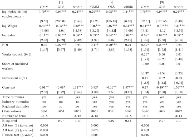
I run all models with four dierent dependent variables: The baseline model estimates the demand for all employees, a second model estimates the demand for highly skilled employees, a third one analyzes the eects of FDI on mod-erately skilled employees (who have a vocational training), and a last model is estimated for unskilled employees.
6.3 Results
Eects of FDI on Total Employment
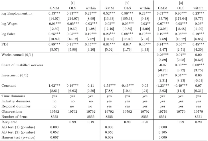
In Table 3 I show the results for 3 dierent specications of the baseline re-gression for all employees including the generated FDI variable. In the rst specication I run a basic model that includes only lagged employment, aver-ages waver-ages, sales, the FDI variable and time dummies. I present the GMM, OLS and within results for all specications. In a second specication I add dummy variables for industry and regional eects. In a third specication, I also include the control variables inXit.5
The results of this baseline model are as expected: I nd a positive eect of the lagged dependent variable, a negative eect of the average wage level and a positive eect of sales. All these variables are highly signicant.6
The generated FDI variable has a signicantly positive impact on the level of employment. This result is not only found in the GMM regression but also in the OLS specication as well as in the within model. In particular the signicantly positive result of the OLS regression emphasizes that the true value of the coecient is positive because the OLS coecient for FDI is biased downwards. The two further specications with dummy variables for industry and regional eects included and with additional control variables lead to the same qualitative results. FDI has a signicantly positive eect on total labor demand. This conrms hypothesis 1a.
Note that standard errors are computed via bootstrapping with 500 replica-tions. This is necessary, because the analytical standard errors may be biased because of the generated FDI variable (Wooldridge 2002, p.116). A comparison between the analytical and bootstrapped standard errors reveals that the boot-strapped standard errors are a slightly larger, but yield the same qualitative results. A further comparison with an estimation without the FDI variable and reliable analytical standard errors (see Table 9 in the appendix) shows that the analytical standard errors in the model with FDI included do not seem to be biased downwards. This suggests that the analytical standard errors may be more precise.
However, dierent test statistics show that the results of the Blundell-Bond estimator may be invalid. The Arellano-Bond test for autocorrelation of rst order rejects the null hypothesis of no autocorrelation at a high level of signi-cance. This is expected, because rst-order correlation of the errors is induced by rst dierencing the data. Therefore, the relevant test is whether the errors in rst dierences are AR(2) or not. This null hypothesis of no autocorrelation cannot be rejected at a signicance level of 5%, but at the 10% level for some
5Table 9 in the appendix present a very basic specication without FDI variables. It shows largely the same results.
6This holds true for almost all dierent specications, estimations methods, and dierent dependent variables (dierent skill groups).
Table 3: Labor demand regression and eects of FDI for all employees
[1] [2] [3]
GMM OLS within GMM OLS within GMM OLS within
log Employmentt−1 0.53*** 0.93*** 0.23*** 0.52*** 0.90*** 0.23*** 0.63*** 0.90*** 0.23*** [14.07] [224.07] [8.99] [13.33] [185.11] [9.18] [15.70] [174.04] [8.77] log Wages -0.06*** -0.05*** -0.03*** -0.05** -0.05*** -0.03** -0.07*** -0.05*** -0.03* [-2.60] [-9.60] [-1.98] [-2.46] [-9.89] [-2.00] [-3.05] [-8.48] [-1.90] log Sales 0.25*** 0.05*** 0.19*** 0.23*** 0.08*** 0.19*** 0.19*** 0.08*** 0.19*** [10.89] [15.12] [7.02] [10.60] [17.00] [7.00] [7.69] [16.72] [6.85] FDI 0.89*** 0.11*** 0.45*** 0.81*** 0.04* 0.46*** 0.74*** 0.06** 0.45*** [5.57] [5.98] [4.20] [5.02] [1.76] [4.33] [4.47] [2.51] [4.20] Works council (0/1) 0.26*** 0.01** 0.00 [3.89] [2.08] [0.52]
Share of unskilled workers -0.07 0.08*** 0.08***
[-0.76] [8.72] [3.75]
Investment (0/1) 0.15** 0.04*** 0.00
[2.31] [8.23] [-0.01]
Constant 1.62*** 0.19*** 0.11 -1.53*** -0.43*** 0.05 -1.23*** -0.49*** 0.07
[8.61] [6.63] [0.50] [7.88] [10.4] [.21] [5.93] [11.4] [0.31]
Time dummies yes yes yes yes yes yes yes yes yes
Industry dummies no no no yes yes yes yes yes yes
Regional dummies no no no yes yes yes yes yes yes
Observations 19792 19792 19792 19792 19792 19792 19779 19779 19779
Number of rms 8555 8555 8555 8555 8551 8551
R-squared 0.99 0.19 0.99 0.20 0.99 0.20
AB test (1) (p-value) 0.000 0.000 0.000
AB test (2) (p-value) 0.052 0.050 0.165
Hansen test (p-value) 0.007 0.008 0.000
GMM estimates are two-step system GMM (Blundell/Bond 1998). Standard errors are estimated by bootstrapping with 500 replications, z-values in brackets. *, **, *** signicant at the 10%, 5%, 1%-level.
Source: IAB Establishment Panel 2002-2007, own calculations
specications. This may weaken the reliability of the results. Furthermore, the Hansen test of overidentifying restrictions suggests that not all instruments meet the requirement of exogeneity. The Sargan test (not reported) comes to the same result. Choosing other lags or instrument sets as well as dividing the sample into West or East Germany didn't improve the test results.
Contrariwise, there are also factors that support the validity of the results. Firstly, in the subsample of the state of Baden-Württemberg the test results proved to be acceptable. The Baden-Württemberg results and those for the complete sample including all German states do not dier systematically. If there is a bias in the results for the entire sample, it is very small. Secondly, I can exploit the fact that the OLS estimator is biased upwards and the within estimator is biased downwards for the lagged dependent variable. The opposite is true for the other regressors. This relation is interchanged if the coecient is negative. That way, I can obtain upper and lower bounds for credible estimates of the real coecients. The unbiased GMM estimator should be in between the
OLS and the within results. The results show that this is true in every case for the lagged dependent variable and in most cases for the other variables. In the few cases when the GMM point estimate lies not in the OLS-within interval, it is not signicantly dierent from one of the two other point estimates. All in all, the GMM results seem to be credible, even if the Hansen test statistic rejects exogeneity of all instruments.7
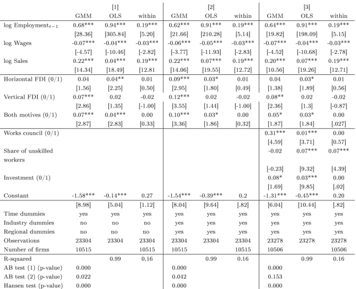
Table 4 presents the results for all employees. In this model, I include 3 dummy variables that indicate dierent motives for FDI. These dummy variables take the value 1 if a rm reports only horizontal investment motives, if it reports only vertical motives or if it reports both kinds of motives, respectively. In this specication, the results for the lagged dependent variable, for average wages, and for sales do not dier in a relevant way from the the specication with the generated FDI variable. The GMM estimator nds positive and mostly signicant eects for rms which reported vertical motives and for rms that reported both motives. The OLS and within results don't support this nding, though. Neither do the GMM estimates of these respective coecient fall into the interval between the OLS and the within results, nor does this interval lie in a signicant range.
Hence, this specication fails to reliably nd signicant eects of dierent kinds of FDI. This may have dierent causes. On the one hand, not all rms with FDI activity also report on their motives. On the other hand, the assumption that the rms didn't invest abroad in the period before 2004 and not after 2005 may be too strict. All in all, hypotheses 1b and 1c cannot be conrmed with this dataset.
7The Hansen test statistic seems not to be highly reliable. For example, in several tests, it suggested that the dummy variables controlling for year-specic eects (which must be exogenous) are endogenous.