EFFECT IN SELECTED COUNTRIES
OF CENTRAL AND EASTERN
EUROPE
Monika B³aszkiewicz
Przemys³aw Kowalski
£ukasz Rawdanowicz
Przemys³aw WoŸniak
The study was financed from the funds of the State Committee for Scientific Research in 2003-2004 within the research project entitled Efekt Harroda-Balassy-Samuelsona w Polsce i innych krajach Europy Środkowo-Wschodniej( Harrod-Balassa-Samuelson Effect in Poland and other Countries of Central and Eastern Europe).
Keywords: Harrod-Balassa-Samuelson effect, Real Exchange Rate, Central and Eastern Europe, EMU
© CASE - Center for Social and Economic Research, Warsaw 2004 Graphic Design: Agnieszka Natalia Bury
ISBN: 83-7178-356-6 Publisher:
CASE - Center for Social and Economic Research 12 Sienkiewicza, 00-010 Warsaw, Poland
tel.: (48 22) 622 66 27, 828 61 33, fax: (48 22) 828 60 69 e-mail: [email protected]
1. Introduction . . . 7
2. The Harrod-Balassa-Samuelson Model. . . 10
3. Empirical Studies . . . 14
4. Presentation of the Data . . . 20
4.1. Data Sources and Definitions . . . 20
4.2. Data Description . . . 22
4.3. Unit Root Tests . . . 23
5. Empirical Verification of the Basic Assumptions of the HBS Model . . 25
5.1. Sector Division and Measurement of Prices . . . 25
5.2. Wage Equalisation. . . 30
5.3. Purchasing Power Parity . . . 36
6. Panel Estimations of the HBS Effect . . . 44
6.1. Models and Cointergration Tests . . . 44
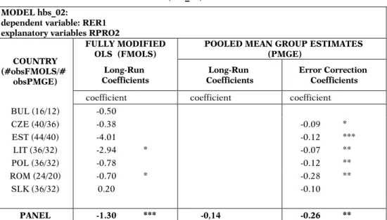
6.2. Estimations of the HBS Equations . . . 45
6.3. Policy Relevance and Estimation of the Size od the HBS Effect 48 7. The HBS and the Distinction between Exchange Rate Regimes . . . 54
7.1. Different Modes of Realization of HBS Effect and the Role of Nominal Exchange Rate . . . 54
7.2. Empirical Verification . . . 58
8. Summary and Conclusions . . . 60
References . . . 62
Tables . . . 66
Figures. . . 80
Monika Błaszkiewicz
She received an MA in International Economics from University of Sussex (2000) and MA in Economic Science from University of Warsaw (2001). Between 2000 and 2002 she worked for the Ministry of Finance (Poland). Since October 2002 she has been a member of the Maynooth Finance Research Group (MFRG) affiliated to the Institute of International Integration Studies (IIIS), based at Trinity College Dublin (Ireland) working on her PhD thesis. Her main field is international macroeconomics; research interests include financial crisis and European integration (EMU). She has collaborated with the CASE Foundation since 2000.
Przemysław Kowalski
Economist at the Organisation for Economic Co-operation and Development (OECD) in Paris since 2002. He graduated in Economics from Universities of Warsaw (MSc), in International Economics from the University of Sussex (MA) and is a PhD candidate in Economics at the University of Sussex. His areas of interests include: international trade theory and policy, applied methods of trade policy analysis as well as macroeconomics and international finance. He has been collaborating with CASE since 1999.
Łukasz W. Rawdanowicz
He holds two MA titles in economics from Sussex University (UK) and Warsaw University (Poland) and pursues PhD research on equilibrium exchange rates at Warsaw University. His main area of interest is applied international macroeconomics. He dealt with issues related to trade liberalisation, currency crises propagation, exchange rate misalignments and exchange rate regime choice primarily from the perspective of transition economies. He worked for the Center for Social and Economic Research (mainly on forecasting) and the OECD (on structural issues). Currently, he is an economist at the European Central Bank.
Przemysław Woźniak
He holds MA (1997) and PhD (2002) in economics from Warsaw University and has studied at the University of Arizona (1995-1996) and Georgetown University (1998-1999) in the United States. His areas of interest include issues related to inflation, core inflation and monetary policy (his PhD dissertation is entitled "Core Inflation in Poland"). He coordinated and participated in numerous research projects in the CASE Foundation. His work experience includes two internships at the World Bank in Washington DC and working in Montenegro as economist for the quarterly 'Montenegro Economic Trends'. In 2001 he was a Visiting Scholar at the International Monetary Fund in Washington DC (GDN/IMF Visiting Scholar Program). He has collaborated with the CASE Foundation since 1996 and became Member of the Council in 2004.
This study investigates the HBS effect in a panel of nine CEECs during 1993:Q1-2003:Q4 (unbalanced panel). Prior to estimating the model, we analyze several key assumptions of the model (e.g. wage equalisation, PPP and sectoral division) and elaborate on possible consequences of their failure to hold. In the empirical part of the paper, we check the level of integration of the variables in our panel using the Pedroni panel-stationarity tests. We then investigate the internal and external version of the HBS effect with the Pedroni panel-cointegration tests as well as by means of group-mean FMOLS and PMGE estimations to conclude that there is a strong evidence in support of the internal HBS and ambiguous evidence regarding the external HBS. Our estimates of the size of inflation and real appreciation consistent with the HBS effect turned out generally within the range of previous estimates in the literature (0-3 % per annum). However, we warn against drawing automatic policy conclusions based on these figures due to very strong assumptions on which they rest (which may not be met in near future). Finally, following the hypotheses put forward in the literature, we elaborate and attempt to evaluate empirically the potential impact of exchange rate regimes on the magnitude of the HBS effect.
Niniejsze opracowanie bada efekt HBS w 9. krajach Europy Środkowo-Wschodniej (EŚW) w okresie 1993:Q1-2003:Q4 (panel niezrównoważony). Przed estymacjami modelu, analizujemy kilka kluczowych założeń modelu (np. o wyrównywaniu się płac, parytecie siły nabywczej czy o podziale sektorowym) i zastawiamy się nad potencjalnymi konsekwencjami ich niespełnienia. W części empirycznej sprawdzamy stopień integracji zmiennych w naszym panelu wykorzystując panelowe testy stacjonarności Pedroniego. Następnie badamy wewnętrzny i zewnętrzny efekt HBS za pomocą panelowych testów kointegracji Pedroniego oraz estymacji metodami group-mean FMOLS oraz PMGE, które dostarczają silnych dowodów na istnienie wewnętrznego HBS, ale nie dają jasnych wyników co do zewnętrznego HBS. Nasze
Abstract
szacunki skali inflacji i realnej aprecjacji związanej z efektem HBS okazały się zbliżone do wcześniejszych szacunków innych autorów (0-3% w skali rocznej). Przestrzegamy jednak przed automatycznym wykorzystywaniem tych szacunków w polityce gospodarczej, gdyż są one oparte na bardzo mocnych założeniach (których spełnienie nie jest pewne w bliskiej przyszłości). Na końcu zastawiamy się nad hipotezami, które pojawiły się w literaturze przedmiotu, zakładającymi potencjalny wpływ reżimów kursowych na skalę efektu HBS oraz podejmujemy próbę empirycznego oszacowania tego wpływu.
Since the beginning of the transition process, Central and Eastern European countries (CEECs) have experienced relatively high inflation rates and substantial appreciation of their real exchange rates. While in the early 1990s, inflation was mainly reflecting price liberalisation, sizeable adjustments of administrative prices and monetary overhang – the legacy of the socialist system1– the inflation performance in recent years can no longer be attributed to those early-transition phenomena. It is widely argued that the positive inflation differential and trend appreciation of currencies in CEECs vis-à-vis most Western economies may be explained (at least to some extent) by structural factors. The Harrod-Balassa-Samuelson (HBS) effect, which links the inflation differential and real exchange rate movements to productivity growth differentials, gained a prominent role among these factors. The HBS theory offers a supply-side explanation of higher inflation and the associated real exchange rate appreciation in countries experiencing higher relative productivity growth. In its domestic version relative inflation in a given economy is explained by relative productivity growth between the tradable and nontradable sectors. It has been observed for some time that the tradable sector usually enjoys higher productivity growth than the nontradable sector (for example, in Baumol and Bowen, 1966). If wages equalise between sectors, higher productivity-driven wages in the tradable sector push wages in the nontradable sector above levels commensurate with its productivity gains. This in turn drives prices of nontradables up and raises the ratio of nontradable to tradable prices. In a two-country setting the HBS effect predicts that the country with higher sectoral productivity-growth differential will experience higher relative inflation (or, higher absolute inflation levels if tradable inflation differential is assumed to be zero).
In the international context the causal link between relative productivity and relative prices can be further used to explain real appreciation of the exchange rate of a country with higher
1Monetary overhang was built over the years in the form of forced savings across socialist economies as a
relative productivity growth. Assuming that the law of one price holds in the tradable sector, the productivity-driven inflation differential will result in appreciation of the real exchange rate deflated with any measure of inflation containing the tradable and nontradable component. Therefore, in view of the fact that each of the three effects related to the HBS theory (rising relative productivities, relative prices and real appreciation of exchange rates) has been observed in the CEECs, it is not surprising that the HBS hypotheses have attracted a lot of attention in the regional context. Higher growth rates of real GDP and productivity in CEECs are to some extent a natural consequence of the transition from highly regulated economies, where productive resources were employed in less than fully efficient manner, closer to their natural level. Another plausible hypothesis is that the process is triggered by convergence, where growth rates differentials ensue from large income and productivity disparities between the region and its Western European neighbours and are facilitated by their progressively closer economic integration. While substantial gains in this process have been achieved already, there still seems to be a sizeable room for convergence and the relative productivity growth differentials are expected to persist for many years in the future. Additionally, as a consequence of the EU accession of eight CEECs as well as the debate on the adoption of the euro, the HBS theory has become a popular framework used for an assessment of the feasibility of meeting the Maastricht criteria. It has been argued that simultaneously setting the ambitious inflation and exchange rate stability criteria, as is the case in the Maastricht Treaty, might be in conflict with the underlying trend of productivity growth. The posited inappropriateness of combining the two criteria stems from the general prediction of the HBS theory that certain productivity growth differentials can result in violating any joint criterion on inflation and nominal exchange rate. The productivity-driven excess inflation and real appreciation should be viewed as a natural equilibrium process in faster-growing economies which in principle does not call for policy intervention. Thus, investigation of the HBS effect in transition economies is of a key importance from the point of view of EMU accession. An evaluation of this effect can shed empirical light on potential problems associated with meeting the Maastricht criteria. It can also provide guidance in choosing the central parity and managing the exchange rate in the ERMII period.
Related to the question of meeting the joint inflation-nominal-exchange-rate criterion is the issue of the posited trade-off between nominal convergence implied by the Maastricht criteria and the real convergence manifested by the GDP catch-up. The problem might arise in the new EU Member States (NMS thereafter), if the inflation and nominal exchange rate consistent with the Maastricht criteria are impossible to achieve in the presence of the sizeable HBS effect. A monetary tightening that might be necessary to bring inflation (or exchange rate) to the Maastricht-consistent level could also suppress real growth. Consequently, there would be a risk of sacrificing the real convergence for the nominal one.
The high policy relevance of the above-mentioned issues has spurred interest in empirical research of the HBS effect in CEECs. The existing literature contributions differ considerably in their methodological approaches as well as country and time coverage. While most of them detect that the HBS effect is indeed at work in CEECs, they usually conclude that observed inflation differential and a real exchange rate appreciation is only in small part explained by the HBS effect. Additionally, the estimates of the HBS-consistent inflation and real appreciation differ considerably suggesting the productivity-driven real appreciation in the range of 0-3% per annum.
Against this background, we seek to reassess the HBS model for CEECs and to contribute to the empirical literature on this topic. The HBS theory rests on restrictive assumptions and their violation can be one of the factors explaining the fragility of empirical estimates. In the presented study we undertake a detailed investigation of the extent to which several key assumptions of the HBS theory (such as wage equalisation or PPP) hold in our panel. Subsequently, we verify the HBS hypotheses using quarterly panel data for nine CEECs during the period 1995-2003. In doing so, we include two alternative versions of the sectoral division and various alternative definitions of key model variables. This is motivated by theoretical controversies and practical problems related to dividing the economy into tradable and nontradable sectors as well as by robustness checks. In addition to estimating the internal and external versions of the HBS model we enhance the policy usefulness of these estimates by calculating the size of the HBS-consistent inflation and real appreciation. Finally, following the hypotheses put forward by Halpern and Wyplosz (2001) and Egert et al. (2003) we elaborate and evaluate empirically the potential impact of exchange rate regimes on the magnitude of the HBS effect.
The remainder of the paper is composed as follows. In the second chapter we present a theoretical exposition of the model. Chapter three contains a concise literature review related to HBS effect covering both the selection of early papers from the 1970s and 1980s as well as recent empirical studies devoted specifically to CEECs. Chapter four presents the data used in empirical analysis as well as the results of stationarity tests of the data. In the fifth chapter we investigate the extent to which assumptions of the HBS theory are met in our sample. In particular, we focus on wage equalisation, PPP and the issue of proper sector division. In addition, we elaborate on the possible consequences of violation of these assumptions for both the theoretical analysis of the HBS model and its empirical evaluation. Chapter six presents panel-cointegration tests and estimations of the internal and external versions of the HBS by means of panel regressions. Subsequently, inflation and appreciation consistent with the HBS effect are computed and discussed in the context of their usefulness for inference about the near future (e.g. the EMU membership). The seventh chapter discusses the hypothesis of the potential impact of exchange rate regimes on the HBS effect and presents an attempt of its empirical verification. Chapter eight concludes.
Initiated by Harrod (1939) and formalised independently by Balassa (1964) and Samuelson (1964), the HBS theory posits a relationship between sectoral productivity differentials across countries and patterns of deviations from PPP (i.e., the fact that, abstracting from transition costs, prices of identical goods measured in one currency are not empirically the same across countries, either continuously or over significantly long periods) in order to investigate the implications of such deviations for international real-income comparison. Over the years, however, the processes predicted by the HBS theory have been extensively modelled in studies, which seek to explain the behaviour of real exchange rates. The formal exposition of the HBS model is presented below.2
It is assumed that a small open economy produces two goods: composite traded and composite nontraded and that outputs are generated with constant–return production functions (CRS):
(1) YT= ATF(KT, LT) and YNT= ANTF(KNT, LNT)
where subscripts T and N denote tradable and nontradable sectors, respectively. Parameters A, K and L with TandNsuperscripts assigned stand for productivity, labour and capital in the two sectors in question. Assuming that both goods are produced the total domestic labour supply is constant and equal to L = LT+ LN.
It is further assumed that capital is mobile across sectors and countries (i.e. there are no resource constraints on capital), but labour only domestically. Labour mobility ensures that workers earn the same wage W in either sector, where the numeraire is the traded good (i.e. relative wage). Perfect capital mobility implies that the domestic rate of return
2The formalisation of the HBS model provided in this section extensively draws on Obstfeld and Rogoff
(1996).
2. The Harrod-Balassa-Samuleson
Model
on capital R is fixed to the world interest rate and is exogenous. If R is the world interest rate in terms of tradables, then, under perfect foresight, R must also be the marginal product of capital in the tradable sector. At the same time R must be the value, measured in tradables, of marginal product of capital in nontradable sector (for details see Obstfeld and Rogoff (1996)). Under the assumption of a perfect capital mobility, the production possibilities frontier of an economy becomes linear and therefore technology is the unique determinant of relative prices of tradables in terms of nontradables (PNT/PT).
Thus, the profit maximisation in tradable and nontradable sectors implies:
(2a) R = (1-γ) AT{KT/ LT}-γ and
(2b) R = (PNT/PT)(1-δ) ANT{KNT/ LNT}-δ
(3a) W= γAT{KT/ LT}1-γ and
(3b) W = (PNT/PT)δANT{KNT/ LNT}1-δ
where γand δare labour’s share of income generated in the traded and nontraded sector, respectively.
Equations (2a&b)-(3a&b) fully determine the relative price of tradables to nontradables with an important implication that for a small country, the relative price of T and NT is independent of consumer demand patterns. But introducing a nontradable good into the analysis is not enough to violate the theory of absolute PPP. If the two countries had identical production functions and capital was perfectly mobile, prices of nontradables expressed in terms of tradables would equalise. According to the HBS effect, what causes persistent deviation of real exchange rate from its PPP values are differences in sectoral labour productivity.
By log differentiating (2a&b)-(3a&b), a systematic relationship between relative productivity shifts and the internalreal exchange rate (i.e., the price of nontradable good expressed in terms of tradable goods) can be derived:
(4) ∆(PNT/PT) = ∆pNT- ∆pT= (δ/γ)∆aT- ∆aNT
Equation (4) can be interpreted as follows: provided that the inequality δ/γ>=1 holds, faster productivity growth in the tradable relative to nontradable sector will push the price
of nontradables upward. If both sectors had the same degree of labour intensity (δ=γ), then the change in relative prices would be equal to the productivity growth differential. The larger the share of labour in the production of nontradables relative to tradables (δ>γ), the larger the effect will be. This is the so-called ‘domestic’version of HBS effect and was first introduced by Baumol and Bowen (1966) who looked at historical data of industrialised countries and found that technological progress in service-intensive goods was smaller than in traded-manufactured goods. However, as Froot and Rogoff (1994) argue, the Baumol-Bowen effect is not a sufficient condition to imply the international HBS effect.
The ‘international’version of the HBS effect rests on the assumption that the PPP holds in the tradable sector. The aggregate price level p (in the logarithmic form) can be decomposed into prices of tradables and nontradables (at home and abroad) with weights
ααand 1- αα, where ‘*’ denotes a foreign country:
(5a) p = αpT+ (1 – α)pNT and (5b) p* = α*pT* + (1 – α*)pNT*
The real exchange rate qis the relative price of tradables produced abroad (measured in domestic currency) with respect to home produced tradables (again, all variables are expressed in logarithms), erepresents a nominal exchange rate (and is defined in domestic currency units per foreign currency so that a decrease implies appreciation):
(6) q = (e + p*) – p
Now, substituting both equations (5a&b) into (6) and expressing the result in terms of changes, we obtain:
(7) ∆q = (∆e + ∆pT* – ∆pT) + [(1 – α*)(∆pNT* – ∆pT*) – [(1 – α)(∆pNT– ∆pT)]
If the law of one price for tradables holds,
(8) ∆pT = ∆e + ∆pT*
then by substituting (4) into (7) and using (6) and (8) one can show how the real exchange rate can shift in a response to sectoral productivity changes between home and foreign country:
(9a) ∆pT- ∆pT*= ∆eT+ (1 – α)[(δ/γ)∆aT- ∆aNT] – (1 – α*)[(δ*/γ*)∆aT*- ∆aNT*] or equivalently:
(9b) ∆qT= ∆eT+ ∆pT* - ∆pT= -{ (1 – α)[(δ/γ)∆aT- ∆aNT] – (1 – α*)[(δ*/γ*)∆aT*- ∆aNT*]}
Again assuming that δ/γ>=1 holds (at home and abroad), faster productivity growth in tradable relative to nontradable sector at home than abroad will lead to a rise in the relative price level and therefore to the real appreciation of the domestic currency. As is the case with the ‘domestic’ version of the HBS effect, equation (9a&b) implies that demand plays norole in determining the relative price and therefore the real exchange rate.3
At this stage, it is worth mentioning that there are other theories that try to explain the so-called ‘Penn-effect’, i.e., the tendency for PPP-based real-income comparisons to be systematically biased (Asea and Corden, 1994). These depend largely on assumptions regarding demand. For example, Kravis and Lipsey (1983) and Bhagwati (1984), building on imperfect capital mobility, heterogenous tastes and factor endowments between countries, draw a conclusion that is the same as the one drawn from the basic HBS effect.
3Given that we can expect a large number of individual tradable goods (i.e. T
1and T2) we can extend the
HBS model to the more general case in which there are additional factors of production (for example skilled and unskilled labour) without invoking demand restrictions. This is the case because for demand to have no role in determining relative prices, the perfect capital mobility is essential administracyjnych.
This chapter provides an overview of the literature investigating both the PPP puzzle and real exchange rate behaviour in the HBS framework. To provide a more complete research perspective the chapter distinguishes between the general literature on the HBS effect and its applications to CEECs.
Drawing on the early work of Ricardo and Harrod, Balassa (1964) and Samuelson (1964) point to the fact that divergent international productivity levels could, via their effect on wages and domestic prices of goods, lead to permanent deviations from the absolute version of PPP due to Cassel (1916). In his seminal paper, Balassa tests the relationship between price levels and GDP per capita and finds a positive relationship between countries’ income and prices. This positive relationship leads him to conclude that this is why the cost-of-living
PPP tends to bring about a spurious overvaluation of currencies of higher income countries. He further states that if international productivity differences are greater in the production of tradables than in the production of nontradables, the currency of the country with high productivity increases will be overvalued in terms of PPP. Consequently, the ratio of PPP to the exchange rate will be an increasing function of income.
Thus, the HBS theory is an appealing and relatively simple theoretical explanation of trends in real exchange rates.4A pertinent question is therefore how useful an explanation of trends in relative prices and real exchange rates the HBS theory really is? Unfortunately, empirical studies are rather inconclusive and many of them point to the limitations of the theory offering competing rationalisations. Also, arguing that demand shifts affect the composition of output, many researchers add additional variables to the basic HBS model. It should be born in mind however that, as an anecdote states “while all models are wrong, some are useful”. This question is the main motivation behind extensive empirical literature discussed concisely below.
The 1980s studies of the HBS effect confirm that it is indeed at work. Hsieh (1982) verifies
4Obstfeld (1993) develops a formal model in which real exchange rates contain a deterministic trend.
3. Empirical Studies
the existence of the HBS effect using the time-series approach Focussing on determinants of the real exchange rate in Germany and Japan against their respective trading partners between 1954 and 1976, Hsieh finds that the productivity-differential variables are significant and have the correct sign. Martson (1987) uses OECD data and calibrates a model of the yen/dollar real exchange rate over the years 1973 to 1983. His findings confirm that labour productivity differentials between traded and nontraded sectors play a positive role in explaining the long-run trend appreciation of the yen against the dollar. HBS studies of the early 1990s detect a somewhat more tentative evidence of the link between productivity disturbances and real exchange rates. Froot and Rogoff (1991) do not find a strong support for the traded-goods sector productivity growth differential and the real exchange rate movements across EMS countries for years 1979 to 1990. Also, Ito et al. (1997), who assess the validity of the HBS model for a number of ASEAN countries, find that although there is some evidence that these countries move in the direction indicated by the HBS effect, the real exchange rate did not appreciate or appreciated only slightly. Furthermore, they cannot find support for the assumptions behind the HBS effect including the law of one price in the tradable sector or the pattern of nontraded versus traded price movements consistent with the evolution of the real exchange rate.
The notable exception is a study by Heston et al. (1994) who, working with the extended data developed by Gilbert and Kravis (1954),5find strong HBS effects across countries and time (i.e., the difference between prices of nontradables and tradables changes with income). Canzoneri et al. (1999) – another exception – test a panel of 13 OECD countries using FMLS estimator. They divide their study into two parts: first they test the ‘domestic’version of HBS, and then look at the crucial assumption of the PPP in the traded sector. Their results show that the relative price of nontraded goods indeed reflects the relative labour productivities in the traded and nontraded sectors. However, the evidence is somewhat mixed when it comes to PPP in the traded sector. Although, PPP seems to hold when DM exchange rates are examined, it shows large and long-lived deviations when US dollar exchange rates are considered.6
A further range of studies point out that real exchange rates could be affected by other real and macroeconomic factors than the HBS mechanism. In terms of these studies, the HBS effect, real interest rate differentials (i.e., interest rate parity), net foreign assets (in portfolio balance models), government spending, and GDP per capita all, individually and together, play a role in determining real exchange rates.
5Originally, it was Gilbert and Kravis (1954) who developed price level measures for common baskets of
goods across countries.
6It should be noted in general that it is somewhat difficult to compare the results of these kinds of studies.
This is because the empirical literature includes a wide range of approaches to explain the HBS hypothesis, and very often departs from its basic Ricardian framework.
For example, Asea and Mendoza (1994) apply a dynamic-general-equilibrium model to disaggregated data for 14 OECD countries between 1975 and 1990 in which they explicitly take into account tastes, technology and endowments. They do it in order to take into account microeconomic factors specified in the original formulation of the HBS model in the Ricardian framework. Their results support the proposition that sectoral differences in productivity growth help explain the trend rise in relative prices of nontradables within OECD countries. However, they find less empirical support for the overall HBS effect – i.e., there is little evidence that long-term differences in the level of the real exchange rate reflect differences in the relative price of nontradables.
De Gregorio and Wolf (1994) base their study on a sample of 14 OECD countries from 1970 until 1985 to examine the joint effect of productivity differentials and terms of trade movements on a real exchange rate and the relative price of nontradables. The main purpose of the joint analysis is to solve the omitted variable problem. They also show how their results are affected if the key assumption relating to international capital mobility is lifted. They find that productivity differentials across sectors are very significant determinants of real exchange rate fluctuations, but not of changes in the relative price of nontradables (terms of trade changes are significant in both cases). Furthermore, they include real income per capita and government spending in their specification. As these regressors capture demand effects and come out highly significant, De Gregorio and Wolf (1994) question the perfect capital mobility assumption of the HBS effect.7
The HBS effect: CEECs focus.
Even if the HBS effect was originally developed to unveil the PPP puzzle, equation (9) is crucial to the better understanding of whythe currencies of CEECs appreciate in real terms once these economies liberalise their markets and why the relative tradables productivity growth differentials between the NMS and the euro area might lead to structurallyhigher inflation once they lock their central parities to the euro.
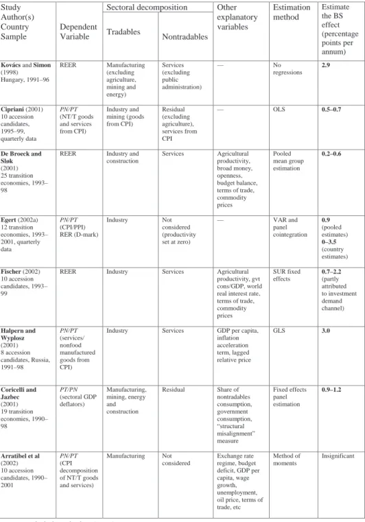
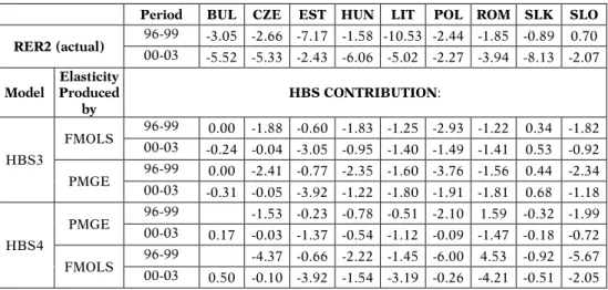
Table 1 presents the differences in results of the key studies of the HBS effect in CEECs and describes the estimation methods applied.
Jakab and Kovacs (1999) use a structural VAR model on Hungarian data over 1993 to 1998 to test the hypothesis that the real exchange rate appreciation in transition economies reflects productivity gains in the tradable sector (they use the real effective exchange rate as a measure of real exchange rate). They find a strong support for the HBS effect amounting to about 2.9 percentage points per year. This result could speak against the EMU participation. For example, sustaining a stable nominal exchange rate could result in the inflation rate of 2.9 percentage points above that of the euro area.
7 For other examples see also Bergstrand (1991), Obstfeld and Rogoff (1996), Balvers and Bergstrand (1997),
Cipriani (2000) focuses on structural inflation rather than exchange rates in his study on the HBS effect. He examines a panel of ten CEECs between 1995 and 1999 using quarterly data. The dependent variable in the estimated regression is the relative price of nontradable goods (i.e., he measures the Baumol-Bowen effect). Cipriani (2000) concludes that productivity growth differentials between tradable and nontradable sectors are not substantial, and argues that it can only explain around 0.7 percentage point of observed inflation.
De Broeck and Slok (2001), test the presence of the HBS effect in the two groups of transition countries: 1) the EU accession countries and 2) the other transition countries. They use the Pooled Mean Group estimator (PMGE) – due to Pesaran, Shin and Smith (1999) – and test the impact of different productivity measures in the tradable and nontradable sectors on the real effective exchange rate during the period 1991 and 1998. The tradable sector is proxied by industry and construction, while nontradable - by services. However, in order to control for macroeconomic development, which can also cause real exchange rate disturbances, they include additional variables like agriculture productivity, broad money, openness, government balance, terms of trade, and the index of fuel and nonfuel prices. The result of their analysis provides a clear evidence of the HBS effect in the NMS, with somewhat less evidence in other transition countries, Russia and other former Soviet Union countries. They suggest that further income catch-up will be associated with further appreciation of the real exchange rate of around 1.5% per annum. Unfortunately, their use of trade-weighted exchange rates calculated by the IMF is problematic because trading partners continue to change over time and include countries from outside the euro area. Moreover, the very short time span of annual data and a large number of explanatory variables makes the quality of the PMGE estimation questionable.
Halpern and Wyplosz (2001) modify the HBS model so that it is more relevant to transition countries. They achieve this by adding demand side variables and argue that it is the catching-up process (i.e., real convergence) that largely drives economic growth in these countries. They provide direct estimates of the HBS effect for all the transition economies for the period 1991 to 1999 using the methodology developed by De Gregorio et al. (1994). As there are many missing observations, they estimate the HBS effect using fixed and random effects, OLS and GLS regressions for an unbalanced panel. Their results confirm the presence of the HBS effect, of the magnitude of 3 percentage points per annum. The important contribution of Halpern and Wyplosz study is that they distinguish between different exchange rate regimes in the HBS model.8
Egert (2002) studies the HBS effect in the Czech Republic, Hungary, Poland, Slovakia and Slovenia. Using quarterly data between 1991:Q1 and 2001:Q2, he applies time series and panel cointegration techniques as well as panel group means FMOLS estimator of Pedroni (2001) to test the presence of the HBS effect in those five countries. In addition, he quantifies the impact of the productivity growth differential on overall inflation, and investigates the extent to which it can explain real exchange rate appreciation in the CEECs. He concludes that while the HBS effect seems to be at work and does lead to the real appreciation of currencies, it does not endanger the fulfilment of the Maastricht inflation criteria by theses countries – somewhat in contrast with the previous studies. The drawback to Egert’s study is that he assumes zero productivity growth in the nontradable sector. This assumption may be too strict given rapid (and unequal across countries) productivity growth in the service sector after its suppression during the central planning (see IMF, 2001). Also, he uses Germany as a proxy for the entire euro area, which may further bias his results.
Egert et al. (2002) explore Egert’s (2002) hypothesis about the impact of the regulated prices on the magnitude of the HBS effect. Using Pedroni panel cointegration techniques they estimate the HBS effect in nine CEECs. They focus on a sample spanning from 1995 to 2000 to eliminate the early phase of the transition period, since, in their view, price and productivity developments during that time were mainly driven by initial reforms and not by the HBS effect. Similarly to Egert (2002), they are able to detect that productivity growth in the traded goods sector is likely to bring about nontradable inflation. However, they argue, it is not obvious that these gains will automatically cause overall inflation to go up and cause the real exchange rate to appreciate. This in fact depends on the composition of the CPI basket (i.e., the lower the share of nontradables, the lower will be the impact of relative price on overall inflation) as well as the share of the regulated prices. Furthermore, they cannot find support for PPP in the traded sector. Summing up, their results suggest that the role of the HBS effect in the price level convergence might be limited and that other factors may be important as well.
The conclusion drawn from the studies investigating the HBS effect in CEECs is that although there is a clear and strong evidence for the long-run relationship between the relative productivity growth and the relative price of nontradables (i.e., high productivity growth in tradable sector brings about relative price inflation), the evidence for the relative productivity differential and related movements in the real exchange rate is somewhat mixed. The most recent studies (see De Broeck-Sløck (2001) and Egert (2002)) tend to be more cautious in their estimates and conclude that the HBS effect is likely to cause the real exchange rate appreciation of around 1.5% per year. This is in sharp contrast to the previous works that detected the HBS-consistent annual real exchange rate appreciation of 3% or more. There are probably a few reasons that can explain differences
in estimates. All of these studies employ different econometric techniques and rest on different assumptions (i.e. proxies used for tradable and nontradable sectors, measures of productivity, assumptions about productivity increases in the nontradable sector, nominal exchange rate deflators, etc.). Also, some of them only measure the domestic version of the HBS effect (i.e. the Baumol and Bowen effect); some additionally try to detect demand-side effects. It should be stressed that more recent studies are probably more reliable as they are based on additional observations and therefore render more accurate results.
4.1. Data Sources and Definitions
Given the exposition of the HBS model and its variants (see chapter 2), their estimations require data on relative prices, relative productivity, and real exchange rates. For this purpose the tradable and nontradable sectors must be defined. Motivated by practical and theoretical considerations of the sectoral division, two alternative definitions of the tradable sector are adopted:
1)with the subscript ‘1’ where the tradable sector comprises industry only, i.e. sections C, D and E of the NACE9 classification of the economic activity (mining and quarrying, manufacturing industries as well as electricity, gas and water supply), 2) with the subscript ‘2’ where the tradable sector comprises industry as well as
agriculture, forestry and fishing, i.e. sections A, B, C, D and E of the NACE classification of the economic activity.
As far as the nontradable sector is concerned, we use a single definition which includes the part of the economy complementing the second definition of tradables, i.e. all sectors except agriculture, fishing, forestry and industry. In line with this division, all remaining variables have two variants: one in which the tradable sector is consistent with definition 1), and the second consistent with definition 2). The complexity of sectoral division at an empirical level will be discussed in more detail in section 5.1.
The data analysed in this study come from various sources. We use quarterly data series with different initial and final observations for various series. Most series, however, start in 1994-1995 and end in 2003. The choice of the sample period was motivated both by data availability and by the conscious decision to eliminate observations from the early 1990s that reflect mostly early transition phenomena rather than long-run relationships (such as
9 NACE is the Classification of Economic Activities in the European Community compatible with ISIC - the
International Standard Industrial Classification of all Economic Activities.
the HBS effect). The data on quarterly Gross Value Added (GVA) and employment by sectors (both in current and constant prices) are taken from Eurostat. In cases of gaps in the Eurostat database we turned to alternative sources. For employment data we used CANSTAT10and prior to 2000 – CESTAT11 while GVA data was sourced from national statistical offices. For data on the CPI and PPI we used the IMF IFS database, while for exchange rates and nontradable component of the CPI we used the OECD Main Economic Indicators database. Whenever these databases had gaps, we used the data from national statistical offices.
Since it is impossible to calculate total factor productivity (TFP) in our sample, we proxy it with average labour productivity:
(10) PRO_Ti_xxx= PRO_NT_xxx=
– average labour productivity in the tradable and nontradable sectors
where VA_Ti_xxxand VA_NT_xxxstand for GVA in constant prices in the tradable (i=1 or 2) and nontradable sectors for a given country (xxx) while EMP_Ti_xxxand EMP_NT_xxx
represent total employment in respective sectors of the same country. Sectoral productivities serve as a basis for calculating relative productivities:
(11) PROi_xxx=
where i refers to the type of sectoral division and takes on values 1 and 2. Relative productivitiy differential, denoted as RPROi_xxx are defined as a ratio of relative productivities in the CEECs and the euro area.
Further, we define three versions of relative price indices:
(12) RPi_xxx= , where i=1 or 2
(13) RP3_xxx=
xxx
PPI
xxx
NT
CPI
_
_
_
xxx
PTi
xxx
PNT
_
_
xxx
NT
PRO
xxx
Ti
PRO
_
_
_
_
xxx
NT
EMP
xxx
NT
VA
_
_
_
_
xxx
Ti
EMP
xxx
Ti
VA
_
_
_
_
10CANSTAT- the Quarterly Bulletin of Candidate Countries complied by statistical offices of the 8 new EU
member states as well as Bulgaria and Romania.
where: PTi_xxx– value added deflator for tradables,
PNT_xxx– value added deflator for nontradables,
CPI_NT_xxx– CPI prices of services (national definitions),
PPI_xxx– producer price index (industry excluding construction).
And finally, below we define the euro real exchange rate in three ways, deflated by the deflator of GVA (RER1), by the CPI (RER2)and by the PPI (RER3):
(14) RER1_xxx=
(15) RER2_xxx=
(16) RER3_xxx=
where: EUR_xxx– nominal euro exchange rate12in country xxx (domestic price of a unit of the euro),
DEF_xxx– Gross Value Added deflator for country xxx,
CPI_xxx– the Consumer Price Index for the country xxx,
PPIM_xxx– the PPIin manufacturing for the country xxx.
The comprehensive information on all names, definitions and sources of variables used in this study are available in Appendix 1.
4.2. Data Description
Figures 1-3 present developments of several indicators of interest for nine CEECs: Bulgaria (BUL), the Czech Republic (CZE), Estonia (EST), Hungary (HUN), Latvia (LAT), Lithuania (LIT), Poland (POL), Slovakia (SLK) and Slovenia (SLO). Additionally Figures 1-2 depict series for the euro area (EUR). The presented series are transformed into logarithms, seasonally adjusted (with the use of the software Demetra), and then scaled with the base period equal to 2003:Q4 (figures 1 and 3) and 2002:Q1 (Figure 2).
xxx
PPIM
EU
PPI
xxx
EUR
_
_
*
_
xxx
CPI
EU
CPI
xxx
EUR
_
_
*
_
xxx
DEF
EU
DEF
xxx
EUR
_
_
*
_
12An increase in the exchange rate means a depreciation of domestic currency. The euro exchange rate prior
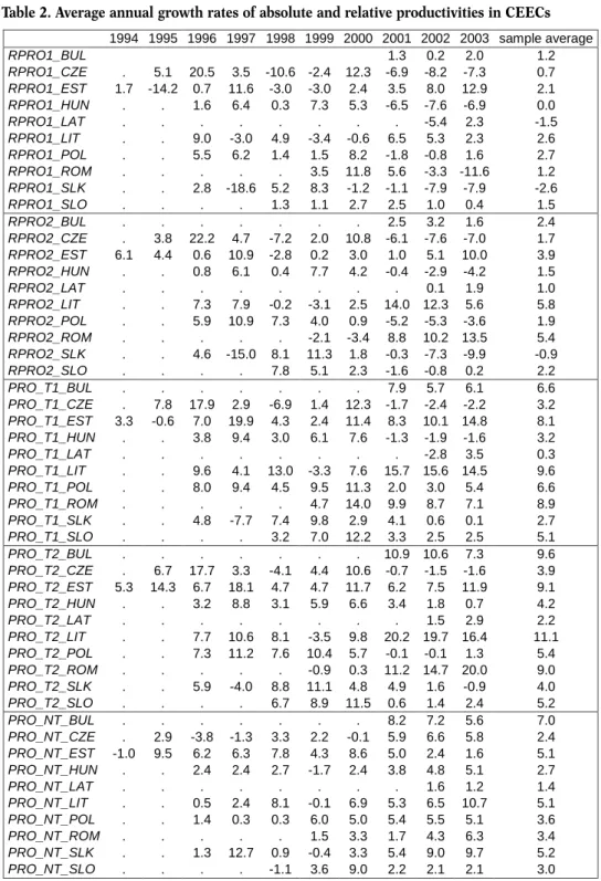
Table 2 and Table 3 present average annual percentage changes of various indicators subsequently used in the empirical part of the paper. The data presented in the table have been based on the ‘raw’ series, i.e. prior to log transformation and seasonal adjustment. Figure 1 presents relative productivity indices, which in line with theoretical predictions of the HBS model, have been on the rise in most CEECs. Due to the generally low share of agriculture in gross value added, the extent of the increase in relative productivities is very similar for both variants of sectoral division and across most countries with the exception of Bulgaria, Slovakia and Romania. This follows from the greater significance of agriculture in generating gross value added in these countries. In Bulgaria, both measures of relative productivity are extremely volatile. In terms of trends, if only industry is considered tradable, one can speak of a slight increase in relative productivities; when agriculture is added to the tradable sector, the trend relative productivity has actually been falling since 2000. In Romania, developments in relative productivities calculated using the sector division of type 1 points to a gradual increase of relative productivity during 1998-2001 and a slight fall afterwards, while productivities calculated using the sector division of type 2 suggest a stable (or slightly falling) relative productivity during 1998-2000, and an increase during 2001-2003. Slovakia presents yet another case: both relative productivity measures are highly volatile, but when smoothed out, point to a stable relative productivity growth.
Relative price indices (Figure 2) have been on the rise for the majority of CEEC during most of the analysed period. For most countries, the definition that exhibits the highest rise is the RP3, i.e. the ratio of price level of services to the PPI. This is particularly pronounced in Estonia (1993-1998), the Czech Republic (1994-2001), and Slovakia (1995-1999). Figures also point to the slowdown of relative price growth in recent years (with an exception of Slovakia where the opposite trend is observed).
As the theory suggests, real exchange rates (Figure 3) have visibly appreciated over the past several years. This trend is particularly pronounced in countries with fixed exchange rate regimes: Estonia, Latvia, Lithuania and Bulgaria. In most countries, in line with declining inflation, the pace of real appreciation has slowed down in recent years and in some of them (e.g. Poland, Latvia and the Czech Republic) the period 2002-2003 saw a nominal and real depreciation.
4.3. Unit Root Tests
Before we proceed to the estimation of the HBS model, we examine our dataset by performing standard tests for unit roots. In line with subsequent analysis, we carry out these tests in the panel framework.
The presence of unit roots is checked by the Im-Pesaran-Shin test (IPS) as well as Levin and Lin (LL) tests. The versions of tests used in our analysis (including the set of critical values) are based on procedures proposed by Pedroni (1999)13. Methodological details on both tests are given in Appendix II. It is worthwhile mentioning that the main difference between those tests is that under the alternative hypothesis, the IPS requires only some of the series to be stationary, while the LL test requires all of them to be stationary (Harris and Sollis, 2003).
Results of both tests are presented in Table 4. Tests were performed on levels transformed into logarithms and after seasonal adjustment for specifications with and without trend (both with a constant).
Most series turned out nonstationary in levels. This result is robust to the inclusion of a trend for all seven price indicators (deflators, CPI and PPI). In the case of specifications with a trend, some tests point to the rejection of the null hypothesis of nonstationarity for all productivity indicators and the euro exchange rate (and the PPI in the case of the IPS test). Thus, the tests are inconclusive in the case of these variables. However, visual inspection of the productivity measures as well as analogous tests applied to the same indicators by other authors (for example, Egert et al., 2003),14lead us to conclude that all (or most) variables are nonstationary in levels. This conclusion motivates an examination of cointegration presented in section 6.1.
13We are grateful to Prof. Pedroni for providing us with RATS codes for his panel procedures.
14Egert et al. (2003) perform the IPS test on a similar set of variables in levels and first differences and
The internal and external transmission mechanisms of the HBS model rest on several restrictive assumptions that were discussed in chapter 2. These assumptions include among others: perfect capital mobility across countries and sectors, free sectoral labour mobility implying economy-wide wage equalisation and the PPP in the tradable sector. On a practical level, an important assumption is a clear division of the economy into two sectors: one producing a composite good which is perfectly tradable in the world markets and the other that produces a nontradable good sold only in domestic markets. Thus, any attempt to empirically verify the HBS effect, necessitates not only testing basic assumption underlying the model, but also calls for the division of the economy into two such sectors. However, at a practical level this is hardly possible and the assumption of two distinct sectors of tradables or nontradables is typically violated as well.
In this chapter we take a closer look at the key assumptions of the HBS theory which may not be met in practice and elaborate on possible implications of their violation for the theory and estimations of the HBS effect. We commence with the sector division assumption, then consider the wage equalisation assumption and finally conclude with the discussion of the PPP assumption.
5.1. Sector division and measurement of prices
5.1.1. Sector division
The HBS theory distinguishes between two separate sectors: one fully open to foreign trade facing externally determined prices (tradables), and one sheltered from foreign competition and producing for the domestic market at prices that are determined domestically (nontradables). As equations (1) through (9) all involve variables
5. Empirical verification of the basic
assumptions of the HBS model
(productivities, wages and price levels) that refer to either of the sectors, a clear and precise sectoral division becomes a very central assumption of the HBS theory.
Therefore, any empirical study, aiming to verify the HBS effect, will inevitably have to address this issue in more detail and make some important judgments. In this section we intend to highlight some consequences of problems related to defining the two sectors and the possible impact of these problems for empirical estimation of the HBS effect. The actual division of the real economy into the tradable and nontradable sectors is a compromise between the guidelines following from the theory, the practice of international trade and the data availability. The measurement problems following from this compromise are further exacerbated by the lack of unanimity among various authors as to the assignment of specific branches of industry into one of the two sectors (e.g. agriculture, mining and quarrying, energy sector etc. are particularly problematic). Furthermore, in view of the high share of services in the foreign trade flows of many countries, the common assumption of nontradability of services is highly problematic as well.
In general, problems related to the sectoral division fall into two closely interrelated categories. In the first case, the proper assignment of some branches or sub-branches of the economy to either sector is made impossible due to the lack of data at a sufficiently disaggregated level. For instance, this is the case with the energy sector whose tradability can easily be questioned, but in view of the problems with obtaining detailed data at the section level, they are commonly included in the tradable sector (together with other branches of industry). Furthermore, there are many services that are traded internationally and are subject to foreign competition (e.g. air transportation services), but due to the lack of data they are treated as nontradable, together with other purely nontradable services (such as for example, haircutting).
The second category of problems arises at a conceptual level. Even if we are in a position to obtain very precise data at a sufficiently disaggregated level, the problem with sector division would not disappear. This is because tradability of goods and services is a highly disputed characteristic and there is no agreed way to measure it.15Although some authors propose formalised algorithms for distinguishing between tradables and nontradables,16 these methods are not straightforward and are not universally accepted. Moreover, once the division following such an algorithm has been made, frictions to arbitrage (mainly transport costs and trade barriers) could make some goods and services nontradable for some ranges of prices, but tradable otherwise. Consequently, even with an access to very detailed and disaggregated datasets, problems with classifying problematic sections or branches of the economy do not disappear.
15Problems with assigning agriculture to either sector is a good example.
16For instance, De Gregorio et al. (1994) define tradables as those sectors for which the export share in total
While there is a clear distinction between these two problems, at a practical level, their consequences are similar. Once the actual empirical division into two sectors has been made, one can be sure that the part of the economy defined as nontradables will inevitably contain an element of the tradable sector while the part of the economy defined as tradables will contain an element of the nontradable sector.
Figure 4 presents the graphical illustration of the sector division problem. In order to focus the argument, let us assume that the actual tradable segment of the economy is A,
and consequently, that of the nontradable sector amounts to (1-A). Due to poor data availability (insufficiently detailed disaggregation) as well as imperfect knowledge, the empirical division implies a different break-up of the economy: the total tradable sector makes up 100*a% of the economy, while the rest 100*(1-a)% is assigned to the nontradable sector. It has to be mentioned that, in reality the value of A remains unknown. If we mistakenly estimate the shares of respective sectors: A and (1-A) as a and (1-a) both estimated shares are ‘contaminated’ and can be expressed as weighted averages of the ‘correct’ and ‘incorrect’ sector (see Figure 4). The true price levels in both sectors are PT and PNTwhile the estimated price levels, pTand pNTare equal to:17
(17) pT= (1-m) PT+ m PNT and pNT= (1-n) PNT+ n PT
where m and n are coefficients indicating the extent of ‘contamination’ of price level measures in sector T and NT, respectively.
The indicator of interest from the point of view of our research is the index of relative prices RP=PNT-PTand its estimated version:
(18) rp = pNT- pT
If we plug (17) into (18) and rearrange the terms we get:
(19) rp = (PNT– PT)(1-m-n)= RP (1-m-n).
which means that the estimated relative prices are equal to true relative prices corrected for ‘contamination’ of sectors by the factor (1-m-n).
17To simplify algebra and in line with the original formulation of the HBS theory, we assume that we deal
with two composite products and two related prices (i.e. PTand PNTare the only prices in the economy).
If our measure of productivity is likewise improperly measured, we encounter the same problem. To allow for heterogeneity of measurement errors, we assume that the share of ‘nontradable productivity’ in a measure of productivity in the tradable sector (pro_T) equals p, while the share of ‘tradable productivity’ improperly included in the measure of productivity in the nontradable sector (pro_NT) is r.18 By analogy the true relative productivity (RPRO) and the estimated relative productivity (rpro) are related through the ‘correction’ factor:
(20) rpro = RPRO (1-s-r)
If we estimate a simple univariate equation where relative productivities explain relative prices by OLS (internal HBS, see equation (4)), then, following from the standard formula for the coefficient β=(X’X)-1X’y (where X is the matrix/vector of explanatory variables and y is the vector of a dependent variable) we obtain:
(21)
where β is the resultant coefficient while B stands for the coefficient that would be obtained where both variables measured correctly over the two sectors and m, n, s, rare numbers ranging from 0 to 1 that reflect the extent of ‘contamination’ in measures of sectoral indicators. The bias disappears when the aggregate ‘contamination’ of both indicators is identical, i.e., the sum of shares of improperly assigned sectors is identical for both indicators. Unquestionably, the bias in the series also causes the actual estimates of the standard error to deviate from the estimates that would be obtained if both sectors were defined properly. Without calculating specific estimates of this bias,19we can make a claim that the resulting t-statistics of the regression will deviate from the values of these statistics in the situation of precise sectoral definitions.
In the case of other techniques used in the empirical analysis in this paper, i.e. panel group mean Fully Modified OLS (FMOLS) and Pooled Group Mean Estimation (PMGE),20the correction factor is much more complicated. It remains, however, to be a function of the extent of ‘contamination’ of sectoral indicators.
Thus, this section points out that the impossibility to measure precisely the various
n
m
r
s
−
−
−
−
Β
=
1
1
β
18The scale of 'contamination' of each indicator may be different due to various data sources and related
possibilities to extract sufficiently disaggregated data. However, we assume that this scale is constant in time.
19This estimate is much more complicated than the estimate of the coefficient bias. 20 For methodological details see Appendix II
indicators over the tradable and nontradable sector might introduce a systematic bias in these series and consequently in the resulting estimates of the HBS effects. Therefore, if the empirical definition of the two sectors is problematic, there are reasons to expect problems with the final estimates of elasticities of the HBS effect, such as the bias in the coefficients and unreliable t-statistics.
5.1.2. Price series problems
Furthermore, additional problems may arise if price series cover goods and services whose prices are administratively controlled by the state. As explained in section 2.3, the HBS model assumes that the price level in the tradable sector is fixed by the PPP condition, while the price level of nontradables is determined in the domestic market as a result of profit maximisation by firms faced with the economy-wide wage rate w and sectoral productivity. Thus, the HBS model assumes a price setting process that is essentially free-market and follows from adjusting prices in response to wage and productivity changes.21
The reality of transition economies is quite different. Central and local governments continue to maintain substantive control over many prices in the economy (Wozniak, 2002 and Egert et al., 2003). This is particularly the case for services many of which used to be part of the social safety net during communist times with prices kept at extraordinarily low levels (e.g. utilities, electricity, telecommunication, and transport). Although in the course of the 1990s, prices of many services were liberalised, central and local governments still regulate a substantive portion of the nontradable sector and a somewhat smaller share of the tradable sector.22In most transition economies (and not only) such controls are exercised over large parts of the transportation sector (e.g. railways), rents, postal and telecommunication, health-care and judiciary services. Various types of agencies typically control growth of prices of electricity, gas and hot water (the bulk of the E section of NACE). Furthermore, prices of fuel, alcohol and cigarettes are determined largely by changes in excise taxes set by the government.23
As a result of this regulation, the price setting process is heavily distorted and departs from that assumed in the HBS theory. In reality, it is the administrative decisions and not the labour cost pressure that drive prices up in specific parts of the nontradable and tradable sector and determine the timing and scale of these adjustments. As mentioned earlier, this problem is
21In the HBS theory the process is somewhat more complex as involves solving the system of four equations:
2a, 2b, 3a and 3b.
22For example, the weight of the administratively controlled goods and services in the CPI basket is about
25% in Poland (NBP materials) and 20% in the Czech Republic and Slovakia.
23Excise tax is one of the many factors determining prices of these products, however, in the case of some
particularly pronounced in the case of services. Using the example of the Polish CPI, we can notice a substantial disparity of inflation rates in free-market and regulated services (Wozniak, 2004). During the period 1991-2003 the average monthly growth of prices of unregulated services was 1.6%, and it was 2.1% for administratively controlled services (1.4% for the CPI). On a cumulated basis, this amounts to the annual inflation difference of 6 percentage points on average during this period. The inflation disparity between the two types of services declines as we approach the end of the sample,24however, it still remains positive.
Such a disparity is very common across the CEECs and the Polish example can be considered representative for this process. There are many reasons for the persistence of the positive bias of regulated service prices. In addition to the already mentioned initial undervaluation of many services under the socialist safety net, we can point to a few other factors common for most administratively controlled services. Most of them are generated in companies that are still state-owned monopolies and have gone through a process of gradual restructuring aiming at replacing the obsolete capital stock and achieving cost recovery (e.g. electricity plants, water supply companies, railways).25Their prices are regulated by various regulatory agencies where price adjustment decisions are made taking into account various nonmarket factors, such as national policies vis-à-vis specific industries (including but not limited to privatisation and restructuring processes), concerns over social consequences of price adjustments and purely political factors. In view of the fundamental difference of such a price setting policy in comparison with the market price setting policy, including such ‘problematic’ sectors in the measure of services is bound to introduce bias in the sectoral price index. However, due to insufficient disaggregation of data, we are unable to single out and eliminate these industries from the sectoral price indicators that consequently cover both the free market and the administered portion of both sectors. In doing so, we cannot hope that the assumption about the price setting behaviour in both sectors is met and consequently, we might encounter problems with observing and estimating the effects posited by the HBS theory.
5.2. Wage equalisation
In this section we closely look at the wage equalisation process between tradable and nontradable sectors. The inter-sectoral equalisation of nominal wages is one of the two fundamental assumptions of the HBS model (see chapter 2). Because wage equalisation is
24Partly due to falling overall inflation and partly due to the fact that the bulk of the relative price catch-up
has been attained already for the administratively controlled sectors.
25Additionally, many of these industries have had to comply with restrictive ecological regulations which
a critical transmission channel between productivity differentials and nontradable prices, the failure to find evidence of inter-sectoral wage equalisation can undermine the HBS theory. Before we move to the visual inspection of the data for CEECs, however, the possible implications of the lack of wage equalisation for the HBS analysis are discussed.
5.2.1.Relative wage differential – consequences for the HBS model
Below, we consider the model discussed in detail in chapter 2, but allow wages in the tradable sector to differ from wages in the nontradable sector. Using equations (1) through (3), we first derive the ‘modified Baumol-Bowen’ effect:
(22) ∆(PNT/PT) = ∆pNT- ∆pT= (δ/γ) ∆aT- ∆aNT+ δ(∆wNT- ∆wT)
In equation (22) the price differential between sectors is not solely explained by the supply side of the economy – i.e., productivity differentials – but also by the relative sectoral wage. Thus, if we omitted the last term of equation (22) in our estimation, when in fact it was significant, we would run into the omitted variable problem. In economic terms, this means that the observed inflation differential between nontradable and tradable sectors may be additionally explained by sectoral wage differences. In other words, the differences between the observed price differential and the price differential implied by the productivity developments may be a result of existing differences in sectoral wages. Equation (23) sets out the implication of the violation of perfect labour mobility in the ‘international’ version of the HBS effect (assuming that PPP holds):
(23) ∆pNT- ∆p*T= ∆eT+ (1 – α)[(δ/γ)∆aT- ∆aNT+ δ (∆wNT- ∆wT)] – (1 – α*)[(δ*/γ*)∆a*T- ∆a*NT+ δ* (∆w*NT- ∆w*T)]
Similar to the ‘domestic’ version of the HBS effect, the lack of wage equalisation means that the sectoral wage differences term at home and abroad does not vanish from the equation. Equation (23) can be regarded as a ‘generalised form’ of the HBS effect in which sectoral wages do not equalise. However, this has different implications under different conditions:
1) If δ (∆wNT- ∆wT)>0 or δ (∆wNT- ∆wT)<0 and δ* (∆wNT- ∆wT)=0, then the inability of the HBS effect to explain the observed trend in real appreciation or depreciation of real exchange rates, may result from the existing wage differences between the two sectors under consideration;