The economic consequences of population and urbanization growth in Italy: from the 13th century to 1900. A discussion on the Malthusian dynamics

D

epartment of

E

conomic

S

tudies

“Salvatore Vinci”

University of Naples “Parthenope”

Discussion Paper

No.2/2010

The economic consequences

of population and

urbanization growth in Italy:

from the 13

th

_{century to 1900.}

A discussion on the

Malthusian dynamics

Bruno Chiarini

University of Naples Parthenope

The Economic Consequences of Population and Urbanization Growth in Italy: from the 13th Century to 1900. A discussion on the Malthusian dynamics.

Bruno Chiarini

University of Naples Parthenope

September 2009

Abstract

In this paper we investigate the quantitative relation between population, real wages and urbanization in the Italian economy during the period 1320-1870. In this period the prevailing conditions were those of a poor, mainly agricultural economy with limited human capital and rudimentary technology. However, these centuries witnessed the considerable growth of urban centers, which was not only a significant demographic phenomenon in itself. The multiplication of such agglomerations had a striking influence on mortality and hence on the general course of the economy in this period. We present two main results i) the positive check is strong and statistically significant and it explains an important part of the dynamic of mortality but the other equilibrating mechanism in the Malthusian model -the preventive check- based on the positive relationship between fertility and real wages does not operate; ii) the urbanization process and the flows of rural immigrants which fuelled it, had profound, complex implications on productivity in agriculture and on wages and population dynamics.

Key words: Malthusian dynamics; urbanization; pre-industrial labor productivity; population trend, demographic changes.

JEL: N33; N53; N93; J11; C32

1

University of Naples, Parthenope, Faculty of Economics, Via Medina 40, 80133, Naples, Italy. Mail:

bruno.chiarini@uniparthenope.it. I have benefited from the comments and suggestions of Paolo Malanima, Massimo Giannini.

1. Introduction

Thomas Malthus argued that the low and stationary level of per capita incomes prior to the end of the 18th century, was causally related to the very slight rates of growth in population. This causation works both ways. Higher incomes increased population by stimulating earlier marriages and higher birth rates, and by cutting mortality from malnutrition and other factors (preventive and positive checks). Diminishing marginal productivity also leads to a drop in per capita income for higher populations. This dynamic model implies a stationary population in the long-run equilibrium. In this paper we investigate the relation between population and real wages in the Italian economy during the period 1320-1870. In this period the conditions that seem to prevail are those of a poor, mainly agricultural economy with limited human capital and rudimentary technology. However, these centuries witnessed considerable urban growth, which was not only a significant demographic phenomenon in itself. Expansion of these agglomerations had a striking influence on mortality and hence on the general course of the economy in this period. One of the main results of this paper is that the urbanization process and the flows of rural immigrants which fuelled it, had profound implications on productivity in the agriculture sector and on wages and population dynamics. Starting from preliminary statistical analysis based upon the decennial frequencies data set provided by Malanima (2002; 2003; 2005) and Federico and Malanima (2004), we perform a time series analysis and attempt to study the aggregate relationship between population, urbanization and wages. 2

In order to investigate the attempt of population to equilibrate through negative feedbacks (population growth-decline is followed by upturn-downturn in wages) we undertake two steps. The paper first studies the evolution of the variables and their statistical features in an attempt to understand whether wages and population time series are characterized by stochastic and/or deterministic trends. The nonstationary nature of the series is known to have crucial economic implications. Furthermore, Bailey and Chambers (1993) and other authors claim for England that real wages and population are integrated to a different degree and thus cannot be analyzed in relation to one another. Second, in order to discuss evidence for the classical theory in Italy and hence the nature of shocks to the population-wage relationships, we estimate and simulate VAR cointegrated models. This allows us to study “short-run” impacts, long-run wage-population elasticities, and feedback paths. The role of urbanization is investigated and cast in the wage-population relationship.3

2

Although data pose unavoidably serious problems, there is a large and growing body of literature which studies economic-demographic relations in preindustrial Europe. See Weir (1991); Lee (1997); Lee and Anderson (2002); Malanima (2005); Clark (2006); Craft and Mills (2007). Eckstein et al (1986), Bergtsson and Brostrom (1997) and Nicolini (2006), amongst others, use VAR analysis for investigating on demographic and economic relationships. 3

Obviously a caveat is called for. The history of the Italian economy is orders of magnitude more complicated and dramatic than this simple time series description. Many features of the history of growth are omitted. Of undeniable importance are the evolution of physical and human capital, property rights, new ideas and institutions, and religious constraints to their diffusion, foreign dominance, and many other factors and events. Here we quote the papers in Storia d’Italia (1974).

The objects of this paper are: carry out an aggregate time series analysis in order to test whether the Malthusian hypotheses (aggregate wage-population relationships) fit the observed patterns in pre-industrial epoch, and empirically analyse the role of urbanization and its relationship with the rural labor productivity.4 This aspect is particularly important, since the relatively slow pace of urbanization may be a condition to delay industrialization.

Carrying out empirical analysis on Malthusian hypotheses is important since there is no fully consensus on the Malthus model as a good representation of the economy before the 19th century. Many authors argue that some qualifications should be taken into account.5 In this context, it is important to be sufficiently precise about the main events and historical facts, and it is naïve to suggest that the relationship may be affected by myriad of other factors. We are aware that the observable data (wages, population, output, urbanization rate etc) in the form of time series, have undergone insurmountable difficulties and that they do not correspond to the theoretical variables. Nevertheless, these time series are the only possible candidates for measuring these variables and providing some aggregate results.

Among the main results of the paper we find that a better standard of living (measured as an increase in rural real wages) does not positively affect population: one of the key elements to restore the equilibrium in the Malthusian scheme does not operate in the epoch considered. The second contribution of this paper is to show that the urbanization rate plays a key (and puzzling) role in the falling trend of economic “efficiency”.

The paper is organized as follows. Section 2 discusses the data set. Section 3 analyses the dynamics of population and real wages in agriculture. In this section we study the statistical characteristics of the time series available. Section 4 reports the long-run estimates and short-run dynamics of the real wage-population relationship using a VAR cointegrated model. A theoretical model it is provided to support the empirical results. Section 5 extends the empirical model to include the urbanization rate. A detailed summary of results and implications ends the paper.

2. The data set

Empirical evidence for a long-run economic-demographic equilibrium, as discussed by Classical theory, is investigated using data provided by Malanima (2002; 2003; 2005), where data are reconstructed for population, nominal and real wage rates in both urban (for master masons) and rural contexts (for agricultural workers), GDP and per capita GDP (total and agriculture), prices of agriculture goods; urban population density. Output variables, population and urbanization rates are measured for central-northern Italy. The measure of urbanization used in the models below is the proportion of the population in towns of 5,000 or more.6

As regards the notation used for wage variables, W represents wages in the agriculture sector. To obtain the real aggregate we used the price index for agricultural goods P. In the paper, whenever we refer to wages we mean real wages in the agriculture sector. With regard to output, Y stands for the GDP, Ypc is the per capita output, Yapc is the per capita output in agriculture and Ya the agricultural product. Demographic variables are Pop for population, FLa which stands for the agricultural workforce and Urban for urbanization rates in central-northen Italy from 1300-50 to 1860-70. The measure of urbanization is the proportion of the population in towns and cities of 5,000 or more.

4

See for instance, Goodfriend and McDermott (1995).

5

See Nicolini (2004; 2006) and Allen (2001) amongst others.

6

The data series are in decennial frequencies. The data in ten-year intervals present two problems. First we cannot study short-term interaction but the results will reflect longer term tendencies. Second, the sample size (55 observations) is not large enough to render analysis of subsamples possible. Statistical series on these variables might be thought to lack reliability. Direct and official estimates are available for Italy as well as many other countries from the mid-19th century onward.7 However, analysis of data construction seems accurate, well-documented, and rich in detail with many verifiable assumptions. Moreover, statistical series may be compared with other studies and estimates (see in particular Malanima 2002). That said, it constitutes the best available data set for the period.

3. The Malthusian Dynamics of the Italian economy from 1300-1850

The evolution of the Italian economy from the second half of the 13th century until nearly 1900 is investigated in this section using the measures of wages, output and population variables described above. Since each observation corresponds to 10 years, in this context, of course, the definition of business cycle should be considered different from the common use. Rather, our analysis seeks to identify changes in the slope of the trend series and long cycles. Thus a truly analysis of short term interactions will not be borne out with data at ten year intervals.

3.1 Population and wages

From the population data, some clear phases are discernible with respect to the long-run path of the main economic variables. Figures 1-4 report the evolution of population, real wages and productivity during the period 1320-1870. Weather, harvest, war and epidemics, as well as changes in labor demand, shifted the mortality and fertility, impacting upon wages which in turn have led to changes in population. A sharp population drop took place after the Black Death and the later epidemics. This is accompanied by a rapid increase in real wages which, however, diminished thereafter, when population growth resumed after outbreaks of the plague around 1450. Wages remained low until the 17th century demographic decline and rose thereafter. A sharp decline occurred in the 18th century with a trough being reached at the beginning of the 19th century. Figure 3 shows that a similar picture may be drawn by the per capita output (both using agriculture and total output), although the dynamic of the aggregate productions shows a positive trend (Figure 2). Productivity slowdown is constant for the whole period, although the reduction in per capita-GDP is curbed whenever a decline in the population trend takes place. Figure 4, as expected, shows the perfect evolution between the agricultural labor force and population.

7

8.2 8.4 8.6 8.8 9.0 9.2 9.4 9.6 9.8 -0.5 0.0 0.5 1.0 1.5 2.0 2.5 3.0 3.5 35 40 45 50 55 60 65 70 75 80 85 POP (left axis) War

Figure 1. Population and Agricult. Real Wage

8.2 8.4 8.6 8.8 9.0 9.2 9.4 9.6 9.8 13.2 13.6 14.0 14.4 14.8 15.2 15.6 16.0 16.4 35 40 45 50 55 60 65 70 75 80 85

POP (left axis) GDP

GDP Agric Figure 2. Output and Agricultural Output

8.2 8.4 8.6 8.8 9.0 9.2 9.4 9.6 9.8 4.8 5.0 5.2 5.4 5.6 5.8 6.0 6.2 6.4 35 40 45 50 55 60 65 70 75 80 85 POP per capita GDP per capita Agric. GDP Figure 3. Population and Per Capita Output

8.0 8.4 8.8 9.2 9.6 10.0 3.2 3.6 4.0 4.4 4.8 35 40 45 50 55 60 65 70 75 80 85 POP (left axis)

Labour Force in Agriculture Figure 4. Population and Labour Force in Agriculture

The plots of wages and population series clearly suggest two empirical distinct facts: a) the existence of an inverse relationship between the two variables, and b) the existence of the opposite secular path for real wages and productivity (which decline through the centuries) and population (which grows after the mid-15th century). The standard of living in Italy did not remain constant, but exhibited a sharp downward trend.

This sheds light on an implication (the iron law of wages) of Malthusian theory: over the long run wages are stationary around an equilibrium level whereas population shows a rising trend. In the next section we study this issue in detail. Moreover, Figure 3 testifies to the Malthusian “spectre” of diminishing marginal returns to labor and, hence, diminishing output per worker as population (and labor force, Figure 4) increases due to the fixity of other inputs.8

It is extensively shown elsewhere that until about the 18th century, the population was essentially stationary whereas a radically different trend emerged around 1750. This occurred in other countries. Lee (1980) shows that the real wage in England was roughly the same in 1800 as it had been in 1300.9 More recently, Craft and Mills (2007) claimed that wages ceased to be Malthusian at the end of the 18th century. Nicolini (2006) shows that positive checks disappeared during the 17th century and preventive checks disappeared before 1740. The standard of living was roughly constant for one thousand years, but in Italy, between 1300 and 1900 real wages and per capita income fell whereas the population grew. Finally, the population was far more variable before 1650 than afterward. In the whole sample reported in the plots above, the standard deviation of population around its trend is 3.9%. In the period between 1300 and 1450 it rose to 6.4%; and including two more centuries in the sample it drops to 4.7%. The plagues substantially affected the trend before 1430 and after 1630.

The prediction of the Malthus model that differences in technologies should be reflected in population density but not in standards of living is stressed in the Italian case. As highlighted by Livi-Bacci (1997), new productive technology led to a large increase in population over the centuries without any improvement in the standard of living.10

4. The wage-population model

In the Appendix, we identify the nonstationary nature of our series. The statistics reported in tables A.1 and A.2 seem to suggest that the real wages and population are I(1).

Although we are dealing with two variables and a cointegrating relationship, we use Johansen’s (1995) technique to estimate and test the time series models. This procedure is used for a single equation as a tool for checking the validity of the weak exogeneity hypothesis and to investigate the strength of feedback coefficients to disequilibrium. Our estimation procedure is the following: after setting the appropriate lag-length of the VAR model, we determine whether the system is conditioned on some dummy variable for controlling structural breaks. Then we test for the existence of a cointegration vector, and finally for weak exogeneity of the wage variable. All the variables are in log.

Estimated equations are derived by a two-variable system with one cointegrating equation and a lag structure p. Consider the following VAR (ECM error correction) model, written in the usual notation:11

8

This hypothesis, as is well known, may be contested on the grounds that capital accumulation and productivity growth more than offset the law of diminishing returns. Moreover, parents’ altruism and endogenous fertility theories show that the Malthusian hypothesis may be refuted. See amongst others Becker (1960), the papers in Razin and Sadka (1995), and those in the Handbook of Population and Family Economics series (1997).

9

See also Galor and Weil (2000) and the works quoted therein.

10

See amongst others Kremer (1993), Galor and Weil (2000).

11

(1) 1 1 1 p t i t t t i y_t y y Bz ε − − − = ∆ = Π +

∑

In our case, y is a k-vector and contains two nonstationary variables (possibly I(1)), z is a vector of deterministic variables and

t

ε is a vector of innovation. Ai and B are matrices of coefficients to be estimated. It is well known that if the coefficient of the matrix Π has a reduced rank (r<k=1 the number of cointegrating relations in our case), there exists 2x1 matrices α and β such that

' αβ

Π = where β is a cointegrating vector and α are the adjustment parameters.

We have seen that our series are characterized, other than by stochastic trends, by nonzero means and deterministic trends. In a similar way, the stationary relations may call for intercepts and trends. For the population-real wage model we cannot rule out the following assumption (the level data have linear trends; the cointegrating equation has only one constant): 12

(2) H r( ) :Πy_t−1+Bz_t =α β( 'y_t−1+µ₀)+α⊥(γ₀) -The stationary equilibrium relationship

Estimating the stationary model using decennial data for 1320-1870 produces the following result (estimated standard errors in parentheses):

(3) + ⋅ − ⋅ ) 78 . 1 ( ) 051 . 0 (.335 12.78 0 : 'y pop w β .

The adjustment coefficients for the two variables are

) 058 . 0 ( ) 041 . 0 (0.111; =−0.17 − = _w pop α α

The model has an intercept in the cointegration vector and in the VAR and it is specified for two lags (20 years). The cointegrating vector and the equation residuals seem statistically satisfactory: Trace, and Maximum Eigenvalue tests indicate one stationary relation at the 0.05 level.13

In the equation, g=12.78 is the constant term. The α_w term measures the speed of adjustment of the real wage towards the equilibrium once the model is re-normalized on the wage variable. We reject the hypothesis of a real wage weakly exogenous with respect to the long-run parameters and the restriction (α_w =0) is not binding under the assumption that there is one cointegrating relation. -Long-run “elasticity”

The long-run relation (3) is normalized with respect to pop. The model shows a long-run population-real wage elasticity of 0.335 but a “high” speed of the wage with respect to a disturbance in the equilibrium relation, whereas the estimated stationary relation implies that an

12

As in Johansen (1995), α⊥ is orthogonal to

α

the cointegration space and the constants from the data.

13

It is well known that the critical values provided by Johansen and Osterwald-Lenum are only indicative in such situations (small sample, dummy variables and trends). The VEC residual serial correlation LM test shows that the Null of no serial correlation up to lag 3 is not rejected (LM-stat does not reject the Null of serial correlation at lag 1, 4.29 prob. 0.38; lag 2, 2.41 prob. 0.66, lag 3, 0.74 prob 0.95).

increase in population reduces, in the long run, real wages by almost 3%.14 The result shows a wage which is much more sensitive to changes in population than what emerges from other estimates. For instance, Lee (1987), using a simple regression with decadal data from 1360 to 1790, reports a wage-population elasticity of -1.0 (significant at 0.05%). Lee’s result is conditional upon a quadratic time trend, to allow for a growing demand for labor, and the rate of inflation.15 Once we adopt the first hypothesis (quadratic trend), we are unable to achieve a cointegrating (stationary) relation between the variables: the trend in the VAR is not statistically significant, and the residuals are not white noise (we easily reject the null of first order autocorrelation, and multivariate normal residuals of the bivariate model). Including the inflation rate (decennial changes in prices of agricultural goods or total goods) improves the statistical model and the stationarity of the relationship, and provides a long-run wage-population elasticity of -4.49 (standard deviation of 0.580). However, these “elasticities” are only indicative. Stationary relationships must be interpreted cautiously. The coefficients of the cointegrating relation cannot be interpreted as elasticities, as in the usual sense, even if the variables (as in our case) are in logs, because all the other dynamic relations between the variables which are specified in the VAR model are ignored. The analysis requires that short-term dynamics and intertemporal adjustment processes generated by equilibrium errors are taken into account.16 Impulse response analysis, taking into account the full system, may provide a more reliable conclusion. To this end, below we report on the model’s adjustment coefficients and in the subsequent subsection 4.1, we perform impulse response analysis.

-Adjustment coefficients and dynamics

There are several important features that deserve mention. First, note that in this system population is not Granger-caused by the real wages in agriculture (that is the coefficient of ∆w_t−i,i=1,2 are zero, whereas the lagged ∆pop_{t i−} ,i=1,2 have nonzero coefficients). However, in the error correction model, both ∆pop_t,∆w_tare Granger-caused by the stationary relation βwhich is itself a function of

1 ,

1 t

pop_t− w₋ . Thus, the ECM shows that there is causality in both directions.

A second dynamic aspect to note concerns the size of the adjustment. The lower limit on the adjustment coefficients of -1 implies that there is no distinction between the short run and the long run. In our case, this hypothesis would mean that wage setters eradicate half of the past wage disequilibrium in about one period (a decade). Coming to our estimates, for wages the coefficient

w

α

If a transitory shock impinges upon the determinant of the birth and mortality curves, changing the population equilibrium, ceteris paribus, it would take the population roughly nine decades to restore the equilibrium, whereas it would require less than six decades of declining real wages. Thus, using the Malthusian model, we can claim that the negative feedback loop whereby in the absence of changes in technology (or availability of land) the size of the population will be self-equilibrating, is quite slow.

To show how the adjustment process operates in (3), consider, in simplest form, the lagged equilibrium as specified in the cointegrating vector. Suppose that the perspective of time is t. Thus

14

The real wage long-run elasticity to population changes, yielded by the model, is 2.98.

15

Lee and Anderson (2002) using state-space models found the elasticity of the real wage with respect to the size of population in line with earlier estimates.

16

if β >0 in (3), this means that the economy was not in equilibrium in the last period (decade): population and/or wages have to change:

(4) popt₋₁> g−

ϕ

If population exceeds the target defined by the wage, to keep on target pop must be reduced (and this is consistent with the theory) or wages must be increased. Since the population adjustment coefficient is negative, whenever the population exceeds the target and the economy is not in equilibrium, population reduce.

-Conditioning (Black Death and Urbanization)

A major feature of the data set is the break occurring in population during the Black Death before 1430 and around 1630. In Italy, as well as the rest of Europe, population reached a peak between 1300 and 1350, but declined sharply following the plague after 1348. A slow recovery initiated only around 1430. A further sharp population decline, following plague outbreaks, started in northern regions around 1630 and in 1656-57 in southern regions.17

Conditioning the model on a dummy variable for this exogenous drop in population provides a negative coefficient for the population equation and a positive coefficient for the wage equation (estimated standard errors in parentheses):18

) 11 . 0 ( ) 035 . 0 ( 149 . 0 : . ; 172 . 0 : . = − = − − D black D black Dummy eq Wage Dummy eq Pop

Further conditioning of the model involves the urbanization process.19 Including urbanization as exogenous variable (urbanization rates, percentage of people living in towns), we are able to improve the statistical model and obtain more Gaussian residuals. The coefficient of the “urbanization” variable in the VAR are strongly significant and negative for both equations:

) 209 . 0 ( ) 049 . 0 ( 629 . 0 : ; 126 . 0 : − = − = Urban equat Wage Urban equat Pop

The negative sign does not lend support to the hypothesis that the level of urbanization may be a proxy for the level of technology.20 Urban concentrations probably reduced the resistance of the population to disease, especially to those illnesses which must be restricted to an endemic area, raising the death rate. In the centuries from 1400 and 1700, the multiplications of more or less vast agglomerations of people exercised a profound influence on mortality. Urban centers created a host

17

Malanima (2002) reports a fascinating and dramatic reconstruction of the evolution of the plague and the fatal diseases of the age. When the first Black Death appeared (1348-49), in Italy the population was 12-13 million; the plague killed 3.5 million (about 27-30% of the population). Major diseases were the Black Death and especially bubonic plague (the main cause of death for about 300 years), but also typhus, dysentery and smallpox. Among the vast literature we cite the data reconstructed by Del Panta (1980) and Bellettini (1987). See Helleiner (1967) and Ziegler (1969) for an analysis of the plague in Europe.

18

black

Dummy =(1350-1360=1; 1640=1).

19

See Malanima (2005). Other than the urbanization process, promising results can be achieved by conditioning the model on the temperature series as measured in Crowley (2000). A detailed analysis may be found in Fagan (2000). See also Malanima (2002).

20

of problems (food and fuel shortages, water, housing, sewage and garbage disposal etc.) and were often the starting-point of epidemic waves. The negative sign found in our model is thus consistent with the fact that in cities average mortality was significantly higher than the birth rate. However, the imposed exogeneity of the urbanization rate in the model does not allow us to take into account the dynamic interrelationship with population growth. In the next section a model with endogenous urbanization is estimated and simulated in order to study the whole demographic effect of this phenomenon. Though the negative effect on population is undeniable, a permanent stream of rural immigrants made it possible to maintain the population in urban centers. This acted as a drain on human resources in the country, but we show that they also created favorable conditions for “efficiency” in the economy.

4.1 Simulation Results

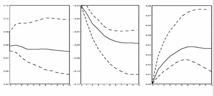
In this section we perform the impulse response analysis of the model discussed above (charts in Figure 5). A shock to a variable of the system not only directly affect the shocked variable, but is also transmitted to all the other endogenous variables through the dynamic structure of the model. In our case, the impulse response function traces the effect of a one-time shock to one of the innovations on current and future values of the wage and population variables. We set the impulses to one standard deviation of the residuals.

Impulse response analysis21 shows that an exogenous increase in rural wages impacts negatively on population dynamics (Figure 5.A). The population response is strongly and significantly negative a decade after the shock and converges to a lower equilibrium.

It is important to assess the relative importance of the specified shocked variables on their own dynamic paths. Interestingly, the direct effect of a positive shock in real wages on its own path shows, after one decade of growth, that real wages reduce toward a new equilibrium, whereas a positive shock in population, pushes up population for the first two decades and, after about 30 years, tapers off toward a new equilibrium. An exogenous increase (fall) in population yields an ever higher (lower) population growth rate for the implicit fall (rise) in real wages. After about 40 years, the growth stops and population decreases (increases) to a new equilibrium.

21

The residual correlation matrix is

          − − = Ω 00000 . 1 0971 . 0 0971 . 0 00000 . 1 w pop w pop

. Confidence Intervals (dotted lines in the

Figures) are obtained with the Hall’s percentile interval bootstrap method. To obtain reliable 95% confidence intervals the number of bootstrap replications has been set to 4000.

Figure 5 A. Response of POP to POP and WAGES (right). VECM Orthogonal Imp-Respo.

Figure 5 B. Response of WAGES to POP and WAGES (right). VECM Orthogonal Imp-Resp.

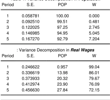
Variance decomposition analysis (Table 1), which separates the variation in an endogenous variable into the component shocks to the VAR, shows that in the first ten years the importance of a wage innovation in affecting population in the VAR is zero. The second period decomposition for the population variable (i.e. twenty years) is due to its own innovation for 99.51 and to real wage innovation for 0.48.

Each time, a negative shock (for instance, the occurrence of a pandemic disease, a war or a reduction in temperature) impinges on population dynamics, wages and production increase. The former tends to remain at a higher level, whereas since productivity of land increases, production tends to increase. Thus, as stressed for instance by Clark (2006), war, banditry, disorder, disease

and even “bad” government (kings) policies, all increase death rates and make societies better off.22 The model simulations appear to be consistent with the stylized facts reported in Figure 3 above. Which factors have determined the swings in population (with a new rapid growth after a sharp decline) and hence in the “efficiency” levels (with low labor productivity after a considerable increase) during the periods is not the aim of this paper. However, with this end in view, in Section 5 we look at the effects of the urbanization process.

Summarizing, the positive check is strong and statistically significant and it explains an important part of the dynamic of mortality but the other equilibrating mechanism in the Malthusian model -the preventive check- based on the positive relationship between fertility and real wages does not operate: population reports a negative and statistically significant response to an increase of real wage.

4.2 A Theoretical Scheme to Interpret the Results

A better income condition does not appear enough to push population upward.23 This result, which we may show to be robust to several modifications of the model, may be justified by several theoretical frameworks.

22

Cipolla (1974) proposes an interesting reconstruction of the evolution from the religious to the rational interpretation of the plague in those centuries.

23

Nicolini (2006) shows how the English demographic system started to move away from Malthusian dynamics well before the Industrial Revolution. Between 1750 and 1810 population levels increased while real wages were not higher

Table 1: Variance Decomposition in Population

Period S.E. POP W

1 0.058781 100.00 0.000

2 0.092510 99.51 0.481

3 0.122025 97.25 2.745

4 0.146985 94.95 5.045

5 0.167270 92.79 7.204

: Variance Decomposition in Real Wages

Period S.E. POP W

1 0.246622 0.957 99.04

2 0.336619 13.98 86.01

3 0.373933 20.32 79.67

4 0.412974 23.90 76.09

i) An exogenous increase in rural wages pushes down the rural labor force and vice versa, as in the classical market-sector economy. This interpretation combines Malthusian and Smithian explanations.

ii) A second interpretative scheme relies upon primitive technology: a shock in rural wages may lead the family with primitive technology to increase its livestock and its storage of harvest and products. Saving reduces population and increases labor force quality. Following the Malthusian scheme, people married earlier when wages were above the equilibrium level and married later when they were below (for instance, Becker 1988). But if the amount of usable land does not increase, and given the presence of infectious diseases that cull many of the children, a wage rise may not stimulate higher birth rates, but may postpone marriage and having children to better times. In this case it does not seem counter-intuitive that households change to a fertility strategy which soon drives income down and increases children mortality. Internalizing the costs of a poor fertility strategy, in the environment of these centuries, would not have been difficult for households.

iii) A variant of the previous interpretation relies upon the so-called “old age security motive” for bringing children. Children are viewed as capital good. Precisely, as the only form of capital for parents to transfer income from their productive years to their old age. When there is an alternative to children for transferring present to future consumption, parents will not invest in children if the return that they yield is lower than the return of investment in capital. Whenever improvements in real wages occur, households are prone to invest in new productive technology or in new methods of exploiting and/or storing seeds and wheat for future crops, or, yet, they are ready to take this opportunity to introduce and disseminate new cereals (maize etc.).24

To support this interpretation we use a very simple overlapping-generation economy to emend the Mathusian model of Ashraf and Galor (2008) (A-G) with the old wage security motive assumption.

Production

There is a single homogeneous good and the production function is a constant-returns-to scale technology, α∈(0,1) with the output produced at time t:

(5) = α 1−α

)

( _t

t kX L

Y

Where L and X are, respectively, labor and land, and k captures the introduction and use of new seeds, better quality of soybean, the use of new methods of cultivation and irrigation, new knowledge for engagement in agriculture an so on. Here there is a first difference with the A-G mode: k is governed, along with the number of children, by parent’ decision. In other words, k may be an alternative to support children as capital. However, to simplify the analysis we may image the parent’s choice problem as a number of children and a fix amount of k. It may be equal the cost of children rearing. Output per worker at time t is

(6) y_t =Y_t /L_t =(kX/L_t)α Preferences

Parent’s and children’s utilities are not linked. The utility function is a Cobb-Douglas function for the parent problem:

than the average pre-industrial level. Nicolini estimates a VAR for data on fertility, nuptiality, mortality and real wages over the period 1541-1840.

24

(7) = γ 1₊−γ 1 t t t c c u

Where c_t is the consumption of an individual of generation t, and γ ∈(0,1), the fraction that the household devotes to consumption. Notice that γ may be interpreted as the importance that the second part of life consumption has in the utility function for the parent. Higher values for γ indicate that the parent is less willing to hedge is second part of life (is less willing to save and invest in children and/or capital).

The production of goods to survive and save in the first period is y_t. The cost of raising a child is

v. Thus each child consume v units of good in each period. The number of the children is n_t and they are view as capital good with return (for each child) equal to (y_t+1−v)=w, where y_t+1 is the production who each of them can provide in the second period, and v is the relative cost. For the sake of simplicity we may assume that for the single parent point of view, this income is given and the net income is w.

In this setup we allow an alternative to children as capital: for transferring consumption to the future, parent may invest in capital and innovation available a that time, to cultivate, store and buy better and new quality of seeds: k increases the effective resources used in production. This investment provide a constant real return r. The budget constraints in the two periods are, respectively: y_t =c_t +nv+k

[

]

From the first order condition, the optimal number of children is: (8) w k r k y v n∗= (1−γ)( _t − )−γ (1+ )

We do not include in the utility function the welfare of each child, therefore, parents’ investments for future consumption will depend on the relative returns. With high costs v and a low return w

population should be reduced. Whenever the capital return (1+r) is higher than the net cost of children the population tends to drop.

Population evolution

The old age security hypothesis determines the population dynamics. The following first order difference equation drives the time path of working population:

(9) _t t t t L w k r k L kX v nL L         + −         −       − = = + ) 1 ( ) 1 ( 1 γ γ α

Here, at time t, parents may invest in new productive technology or in new methods of exploiting and/or storing seeds. Thus output per worker produced at time t is defined by (6). At time t+1 we

maintain the assumption on the exogenous positive net return w. Since ∂yt₊₁ ∂Lt₊₁<0, this is a strong assumption for the dynamic evolution of the economy. However, this hypothesis, which makes more explicit the analysis, does not affect the result.25

For a given k, the unique steady state level of population is (10)     − =     + = Ω Ω + + = − ν γ ξ γ ξ ξα_{( )(1 )} α_; (1 ) (1 ) 1 1 w r k k kX L

In this setup a technological advancement provides a decreases in the steady state level of population: (11) 0 )) ( 1 ( ) ( 1 _<      Ω + + Ω + − = ∂ ∂ ξ α ξ k k X k L

Given the rate of growth g_t+1 =L_t+1−L_t /L_t , a technological advancement provides a decrease of the rate of population growth between t and t+1:

(12) 1 (1 ) 1 (1 ) _<0         Ω − − −       − = ∂ ∂ + − v L X k v k g_t γ γ α α α ,

Notice that the drop in the rate of growth will depend on the relative return Ω. The parents will not invest in children if the return that they think to achieve is lower than the return obtained in the alternative investment, and this will affect the rate of growth of the population.

Also, notice that for a given k, the rate of population growth is lower the lower is the level of the population: (13) 1 (1 )( ) 1 _<0     − − = ∂ ∂ ₊ γ α ₋α₋ α kX L v L g t t

These results compared with those provided by, says, the A-G model, depict an opposite evolution of population to technological advancement. The rise in income per capita (through a rise in k or an exogenous drop in population):

(14) 1 (1 )_>0      ₊ + = ∂ ∂ w r k y ξ γ

may not generate an increase in population, the opposite of the Malthusian assumption. In this literature, a similar result (an increase in income lowers fertility and, therefore population) may be

25

We may achieve these results, relaxing the assumptions on the dynamic evolution of the economy, using some monotonic transformation of the utility function (7).

obtained, under certain conditions, substituting child quantity by child quality (parents invest in terms of education).26

-Criticism

A criticism of this novelty (Granger causality runs in both the ways from population to wages and

vice versa, with a negative relationship) stresses by an historian referee, is that we do not find any increase in population after the rise in wages because of several minor epidemics, especially in the century 1350-1450, struck the Centre and North of Italy. Population stagnates after big epidemics, although wages are high, simply because there are many smaller, but frequent, epidemics (not only plague, but also typhus). The causality wage-population is hidden by the occurrence of these diseases.27 Only the decreasing number of minor epidemics allowed population to grow after about 1450-70; and then long after the Black Death. This should be the reason why high wages do not Granger cause population recovery.

Conversely, we think that the occurrence of epidemics waves (but also social disorder, wars and invasions) support our results for the pre-industrial era in Italy. Consider, for instance, the simple

old age security model reported above, and introduce a probability of survival ρ (or a discount factor) into the utility, ut =γln(ct)+ρ(1−γ)ln(ct₊₁). It is straightforward to predict the effect of mortality on investment: a lowerρ brings lower investments in absolute and relative (children) terms.

For instance, the population drop in the aftermath of the Black Death increases income per capita. In this context the probability of survival is very low and, therefore, is much more likely that people engage in short-sighted behavior, using the rise in income per capita for improving own condition rather than invest in children.28

5. The urbanization effect on the model

In this section, we investigated the effects of urbanization in the wage-employment relationship. In the pre-market period, the appearance and the developments of cities were a condition for industrialization. Economists and historians such as Boserup (1981), Goodfriend and McDermott (1995) and Malanima (2005; 2008), amongst others, have highlighted this aspect, that emerges eloquently from the data. The urbanization figures show as some European countries, which first have abandoned the primitive technology, quickly progressed in the urbanization rate between the 15th and the 17th century. The three countries which played a decisive role in the European economy, each gained dominance in sequence and in parallel to the process of urbanization: Italy (central-northern), Netherlands and England.29

26

For instance, Razin and Sadka (1995), Nerlove and Raut (1997) and Doepke (2006).

27

See amongst others, Del Panta (1980), Del Panta et al (1966).

28

There are, furthermore, big “structural changes” in Italian demographic history not explained by wage movement, but influenced by other important variables: primarily maize’s introduction and spread in 17th-19th centuries; climatic changes. Labour and land intensification play also an important role. As recalled above in footnote 3 the history of the Italian economy is orders of magnitude more complicated and dramatic than this simple time series description. Here, however, we are performing a time series analysis and, following the literature quoted above, we are attempting to study the long-run macroeconomic relationship between wages and population. Many features of the demographic history are omitted because are hard to show or quantify, and the econometric analysis, as we are going to show below, with a more complete model, is quite robust.

29

See Malanima (2002). In particular data reported in Figure 2.17 pg. 91. Of course there are others factors (changes in education, property-rights, preferences across social classes, culture and so on) that have had an impact on economic

In the previous model we captured the negative urbanization process effect on population and the positive effect on rural wages conditioning the VAR model on the exogenous urbanization rate. Such modeling may be misleading given the importance of the causal connection between mortality, rural immigration, wages and productivity in agricultural sector. Moreover, the exogeneity assumption for urbanization made in the previous model amounts to the assumption that wages and population do not Granger-cause the urbanization rate. To deal with this shortcoming, we include the urbanization rate in the model as a further endogenous variable.

After all, the view that the transition from a traditionalist and religious-minded society to the individualistic and mobile world of the market society which originated and developed in towns, has been credited to many authors.30

-Cointegrating space:

The cointegrating space contains an intercept (as in equation 3), and Trace, and Maximum Eigenvalue tests indicate that it is characterized by two stationary relations at the 0.05 level.31

Analysis supports the choice of one common stochastic trend and two stationary relations. The space within which the cointegrated variables move (the attractor set) is now a hyperplane with a dimension determined by the three endogenous variables and two cointegrating relationshis:

(14) 82 . 2 063 . 0 : 27 . 9 473 . 0 : ) 015 . 0 ( ' 2 ) 067 . 0 ( ' 1 − − − + w urb y w pop y β β

We recall that the cointegration vectors cannot be interpreted as representing structural equations because they are obtained from the reduced form of a system where all of the variables are jointly endogenous. Thus, although these relations taken alone as well as each single equation taken alone may seem economically meaningful structures, they are only indicative.

The restrictions on identifying the two separate cointegrating vectors were tested jointly with testing for population, urbanization rate and wages being long-run weakly exogenous for both the stationary relations. The LR test for this joint hypothesis indicates that we can reject these reductions at a 5% level. -Adjustment coefficients: ) 017 . 0 ( 2 ) 004 . 0 ( 1 ) 035 . 0 ( 2 ) 134 . 0 ( 1 ) 120 . 0 ( 2 ) 028 . 0 ( 1 054 . 0 0006 . 0 ; 099 . 0 465 . 0 ; 113 . 0 079 . 0 − = − = = − = = − = ∗ ∗ urb urb w w pop pop α α α α α α

outcomes in a country undergoing the transition from stagnation to growth. See, for instance, Jones (2001) and the survey of Doepke (2006).

30

See, amongst others, Hicks (1969), Hohenberg and Hollen Lees (1985), Blockmans (1989), Tilly (1990). Moreover, in some cases, the boom in urbanization could also be associated to that of the greatest building booms. A striking labor supply which flooded the towns and cities allowed ecclesiastical and military architecture to flourish.

31

The following restrictions identify all cointegrating vectors. In the first cointegrating relation we normalized on the population variable and restricted the urbanization variable to zero. The second cointegrating relation has a zero restriction on population and is normalized on the urbanization variable. The model performs quite well; residuals are stationary. Further tests confirm this hypothesis. The VEC residual serial correlation LM Test indicates that there is no serial correlation up to the lag order of 4, with probabilities that range from 34 to 93%.

The α coefficients relate the error correction terms β₁,β₂ (the long-run) with the first differences (the short-run) of the endogenous variables pop, w and urb. Thus, α_pop1 is the first long-run relation (error correction) in the population equation; α_pop2 is the second error correction described above (β₂) in the population equation and so on. The marked coefficients are not statistically significant. Population and urbanization rate adjustments are rather sluggish whereas wage adjustments to deviations from disequilibria are more rapid.

-Conditioning:

The VAR is augmented by a shift dummy variable to account for the effects concerning the plagues. A second exogenous variable (Temper) is included in the VAR to allow for the temperature effects on the endogenous variables.32 Below we report the coefficient and the standard deviations which are statistically significant for the respective equations:

) 009 . 0 ( ) 155 . 0 ( ) 069 . 0 ( ) 033 . 0 ( 026 . 0 : 2 16 . 0 : ; 367 . 0 ; 146 . 0 : = = − = − = − − Temper equation Urban Dummy equation Wage Temper Dummy equation Pop D black D black

As expected, plagues have a negative short-run effect on population and a positive effect on real wages. The short-run effect of the temperature change is negative for population and positive for the urbanization rate.33

For the population-wages-urbanization system, the innovation correlation matrix (given in Table 2) shows that there are very low correlations among residuals (they are orthogonal) and, therefore, impulse response analysis may be performed.

Table 2. Innovation Correlation Matrix: “Urbanization Model”

pop wage Urban

pop 1.0000 -0.0457 0.0921

wage -0.0457 1.0000 -0.2105

urban 0.0921 -0.2105 1.0000

32

The data set is taken from Crowley (2000), which reports the phases in the temperature of the Northern Hemisphere. However, the inclusion of these data may be a valid approximation. A detailed analysis of climate change for different epochs and their possible effects on the economy is in Malanima (2002).

33

It is not clear how fluctuations in temperature may affect the economy. For instance, in Mediterranean regions, an increase in temperature may give rise to drought and therefore negatively impact on harvesting and population.

5.1 Simulation Results

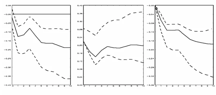
The following plots in Figure 6 show the reaction of each variable to the one standard innovation shock of each other. The dynamic responses of population, rural wages and urbanization rate are depicted, respectively, in Figures 6.A, 6.B and 6.C.

Figure 6 A. Response of POP to POP, WAGES, URBAN (right). VECM Orthogonal I-R.

Figure 6 C. Response of URBAN to POP, WAGES, URBAN (right). VECM Orthogonal I-R.

There are a number of features worthy of comment. i) As in the population-real wage model the response of population to itself provides a new permanent equilibrium level. ii) Analogously to the previous model, after a wage increase, population decreases. Thus, in Italy, before industrialization, the Malthusian income-population feedback is confirmed to be weak; living standards and population growth were not positively related. iii) In contrast with the wage-population model, by allowing the urbanization variable to be endogenous a rise in the urbanization rate provides an increase in population. iv) Both positive changes in population and urbanization entail a drop in

rural real wages. v) The urbanization rate rises after an increase in population size. Thus, after, for instance, a plague, or during a war, death rates increase above birth rates and population size decreases, emptying towns and cities. vi) A further interesting characteristic concerns the dynamic path of urbanization: after a change in the population the urbanization rate slowly converges to the previous equilibrium after about 40-50 years. vii) There is an inverse relationship between rural real wages and the urbanization process: reductions in agricultural wages lead people to leave the countryside and agricultural sectors for towns and new crafts and jobs.

The impulse responses reveal a clear and statistically significant reaction of wage (negative) and urbanization (positive) to a positive shock in population. The reduction in wages along with a decline in agricultural output per worker could not support a context of rising urbanization. The response of rural wages after a positive shock in urbanization rate is negative because an upsurge of urban inhabitants drains farmers and agricultural surplus needed to feed the people that locate in town and cities. This does not allow that the economy will deviate much from primitive production equilibrium.

The explanatory scheme may be compatible with the fact that the negative trend of the urbanization rate in Italy was effectively one of the factors which curbed the transition from stagnation to growth. After a massive urbanization from the tenth century to 1300, the successive epoch, which span from 1300 to 1870, saw a declining urbanization (Figure 7 below). As pointed out by many, the rise of urban population in Europe indicates the extent to which specialization associated with the division of labor accompanied economic development.34

-The urban Dynamics

The model outcomes deserve attention. First, with respect to the wage-population model simulation, the urbanization model shows that the urbanization rate may be one of the factors that determined the swings in population and efficiency levels described by the stylized facts. The mechanism is analogous to the previous model. Now, however, an increase in the population brings about an increase in urbanization rate and a fall in rural wages. Both these effects impinge on labor productivity, reducing rural income and increasing the labor force.

An implication of these results may be described with the help of the model of Goodfriend and McDermott (1995).35 In this framework, per capita product grows as production shifts from primitive processes to market-based specialized techniques, and the pace of this shift reflects the rapid process of urbanization. Their model is based on a market sector characterized by increasing returns to labor and a primitive sector characterized by diminishing returns to labor. When population decreases, the gap between these two economic sectors widens and this allows a unique (corner) equilibrium where the economy remains purely primitive with the whole labor input allocated to the primitive sector. When population and urbanization grow (households grow and move to the cities, abandoning the primitive technology), there may be other equilibria in which households allocate portions of working time in both the sectors. The equilibrium would move as population and urbanization continue to grow, reaching the specialized market economy. To this end, population pressure should induce an acceleration of the pace of urbanization.

By setting the urbanization rate as an exogenous variable (as in the wage-population model) an exogenous increase in urbanization reduces population growth as death rates usually exceed birth rates in towns and cities. The urbanization model reveals a different and much more complex picture. A drop in the urbanization rate raises rural wages and reduces the population. Overpopulated urban centers were periodically struck by epidemic waves, social disorder and

34

Well-known discussions on these issues appear, amongst others, in Goodfriend and McDermott (1995), Bairoch (1988), Hohenberg and Lees (1985).

35

invasions,36 reducing population levels and increasing the real wages in the agricultural sector. Whenever this happened, higher income and a lower population pushed economic efficiency upward (pro capita output). The higher income per head, in turn, meant resources to finance re-population in cities and towns, pushing rural immigrants toward urban concentrations and new crafts and jobs. These people were attracted by the higher urban wages paid in manufacturing and commerce. Thus, the appearance of disease, warfare and famine, which for about 400 years had been the main “agents” of demographic dynamics, were the real engine of this economy.

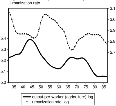
Factors that reduce population lead to high agriculture labor productivity. This means that farm workers may feed many non-farm people living in towns, stimulating urbanization and hence a fall in rural wages, a rise in population and a reduction in the efficiency level of the economy. Thus the demographic relationship and its consequences may be conceived in the following way. Whenever an adverse demographic shock impinges upon population and urbanization, this generates, after some decades, an increase in economic efficiency and hence a new increase in population and urbanization rates. 5.0 5.1 5.2 5.3 5.4 2.7 2.8 2.9 3.0 3.1 35 40 45 50 55 60 65 70 75 80 85

output per worker (agriculture) log urbanization rate log

Figure 7. Trends: Output per Worker in Agriculture and Urbanization rate

Figure 7, indicates that the significant gains in urbanization in Italy after 1470 and 1670 are preceded by increases in output per worker, with the latter following plague years. Our simulation thus explains the urbanization dynamics for the Centre and North of Italy, described in Malanima (2005).37

Of the most important destructive events occurring in the 16th century, we should mention the French sack of Brescia

(1511) and Pavia (1528); in 1527 Rome was sacked by the mutinous troops of the Emperor Charles V, and Spanish troops sacked Genoa in 1532.

37

Following Federico and Malanima (2004) we learn that during the three centuries from 1000 until 1300, Italian agricultural productivity rose by about 20 percent. Then a long period of 600 years followed, from 1300 until 1900, in which Italian agricultural productivity stagnated or slowly decreased.

Concluding Remarks

Wars, disorder, disease, and poor policies of Italian and foreign sovereigns have considerably affected the pattern of death and birth rates and made the flow relationship between the countryside and the town extraordinary complex. From these dramatic outcomes, using imprecise aggregate data we attempted to specify models to explain their effects. The simple models set out in the previous section allow us to perceive a rather complex dynamic relationship between wages and demographic variables. Our main findings are as follows:

-Improvements in productive potential are neutralized by population growth. A large population can be sustained at a constant or even lower real wage. Data and simulations show that over the period from the 14th to the 19th century, increases in the size of the population were absorbed with a deterioration in the rural real wage.

-On examining the responses of our multivariate models, we stress that fertility and mortality did not respond to changes in real wages in a Malthusian way. An increase in real wage does not produce a decline in the death rate or an increase in the birth rate. Rather, our simulations show that there is a statistically significant reduction in population growth. Thus, Malthusian income-population feedback appears to be rather weak. In Italy, before industrialization, living standards and population growth were not positively related.

-Equilibrating tendencies were extremely weak (and slow) in a context where shocks of different nature were large.

-The economy seems to be characterized by primitive aspects which do not allow primitive technology to raise economic efficiency along with a continuous reduction in output per worker. -The urbanization process may be a factor in explaining the empirically observed reduction in efficiency. This result crucially relies on the endogeneity of the urbanization rate. Indeed, conditioning the model on the urbanization rate, as in the wage-population model, provides a negative effect on population.

Appendix

A.1.

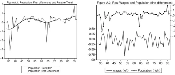
The order of integration of macroeconomic variables has crucial consequences for appropriate modeling of time series data and for proper understanding of the aggregate phenomenon. It is widely acknowledged that the form of nonstationarity in a time series may well not be evident from

examination of the series. Moreover, deterministic rather than stochastic trends have important economic implications. A trend-stationary time series evolves around a deterministic trend, i.e. around some specified and predictable function of time. Conversely, a series with a stochastic trend has no clear long-run pattern, since its longer term movement is affected by stochastic disturbances, which have an enduring effect on the future path of the series. In our context, this means that a shock occurring to the estimated series of population and real wages due, for instance, to weather, harvest, epidemics etc., may have permanent or, conversely, temporary impacts on the long-run movement of the series.

Thus it is essential to identify the nonstationary nature of our series. Statistical inference about a stochastic trend is often combined with a deterministic trend, and it is not straightforward to distinguish between them when several breaks are present in the variables. Furthermore, analysis is complicated by the weakness of the unit root tests when small samples are used.

Trends, whether stochastic or deterministic, may give rise to spurious regressions; they provide, if erroneously identified, uninterpretable or misleading results.To this end, our variables, which seem subject to breaks and to have a peculiar evolution, deserve more attention.

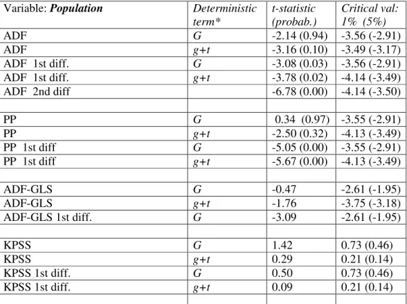
Table A1: Stationarity tests: The Null H0 of Unit Root (H0: stationarity for KPSS)

Variable: Population Deterministic

term* t-statistic (probab.) Critical val: 1% (5%) ADF G -2.14 (0.94) -3.56 (-2.91) ADF g+t -3.16 (0.10) -3.49 (-3.17) ADF 1st diff. G -3.08 (0.03) -3.56 (-2.91) ADF 1st diff. g+t -3.78 (0.02) -4.14 (-3.49) ADF 2nd diff -6.78 (0.00) -4.14 (-3.50) PP G 0.34 (0.97) -3.55 (-2.91) PP g+t -2.50 (0.32) -4.13 (-3.49) PP 1st diff G -5.05 (0.00) -3.55 (-2.91) PP 1st diff g+t -5.67 (0.00) -4.13 (-3.49) ADF-GLS G -0.47 -2.61 (-1.95) ADF-GLS g+t -1.76 -3.75 (-3.18) ADF-GLS 1st diff. G -3.09 -2.61 (-1.95) KPSS G 1.42 0.73 (0.46) KPSS g+t 0.29 0.21 (0.14) KPSS 1st diff. G 0.50 0.73 (0.46) KPSS 1st diff. g+t 0.09 0.21 (0.14)

ADF=Augmented Dickey-Fuller; PP= Phillips-Perron; DF-GLS=Elliot-Rothenberg-Stock DF-GLS; KPSS=Kwiatkowski-Phillips-Schmidt-Shin test; Note that the KPSS test output provides the asymptotic critical values tabulated by the KPSS. The series is assumed stationary under the null hypothesis. The PP test uses an alternative method of controlling for serial correlation when testing for a unit root. The DF-GLS test modifies the ADF. Data are detrended in the presence of a constant and/or linear trend. * In the tests, g is a constant and t is a deterministic linear trend.

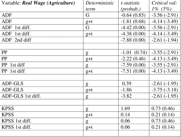
Table A2: Stationarity tests: The Null H0 of Unit Root (H0: stationarity for KPSS)

Variable: Real Wage (Agriculture) Deterministic term t-statistic (probab.) Critical val: 1% (5%) ADF G -0.64 (0.85) -3.56 (-2.91) ADF g+t -1.81 (0.68) -4.14 (-3.49) ADF 1st diff. G -4.42 (0.00) -3.56 (-2.91) ADF 1st diff. g+t -4.38 (0.00) -4.14 (-3.49) ADF 2nd diff -7.88 (0.00) -2.61 (-1.94) PP g -1.01 (0.74) -3.55 (-2.91) PP g+t -2.22 (0.46) -4.13 (-3.49) PP 1st diff g -7.59 (0.00) -3.55 (-2.91) PP 1st diff g+t -7.51 (0.00) -4.13 (-3.49) ADF-GLS g 0.39 -2.61 (-1.95) ADF-GLS g+t -1.86 -3.75 (-3.18) ADF-GLS 1st diff. g -3.82 -2.61 (-1.95) KPSS g 1.69 0.73 (0.46) KPSS g+t 0.14 0.21 (0.14) KPSS 1st diff. g 0.06 0.73 (0.46) KPSS 1st diff. g+t 0.06 0.21 (0.14)

ADF=Augmented Dickey-Fuller; PP= Phillips-Perron;

DF-GLS=Elliot-Rothenberg-Stock DF-GLS; KPSS=Kwiatkowski-Phillips-Schmidt-Shin test; For a comment see Table A.1.

Following the Choi and Yu (1997) approach, we test sequentially I(0) versus I(1) and I(1) versus I(2) if the first hypothesis is rejected, taking into account drifts and deterministic trends in the data. a) Results from ADF, DF-GLS, PP and KPSS test are reported in Table A.1 whereas Table A.2 reports the relative tests for real wages. As is evident, all tests fail to reject the null hypothesis of a unit root in the time series at 5 percent significance level, implying that the levels of population and real wages are non-stationary. Notice that the ADF test for both real wages and population may appear less clear, but we can reject the non-stationarity of the series at first differences. This is an important issue, since the log of a variable which is I(2) will have an I(1) growth rate; thus a shock to the series will result in persistence in the growth rate and level of the series. Alternatively, some evidence of a deterministic trend in the data may emerge from the tests.

b) However, it should be borne in mind that it is not easy to operate for such discrimination between an I(2) model, a model with a deterministic trend in the data and a model with a structural break. As