Tutz, Binder:
Boosting Ridge Regression
Sonderforschungsbereich 386, Paper 418 (2005) Online unter: http://epub.ub.uni-muenchen.de/
Boosting Ridge Regression
Gerhard Tutz1 & Harald Binder21Ludwig-Maximilians-Universit¨at M¨unchen, Germany
2Universit¨at Regensburg, Germany
July 2005
Abstract
Ridge regression is a well established method to shrink regression parameters towards zero, thereby securing existence of estimates. The present paper investigates several approaches to combining ridge regression with boosting techniques. In the direct approach the ridge estimator is used to fit iteratively the current residuals yielding an alternative to the usual ridge estimator. In partial boosting only part of the regression parameters are reestimated within one step of the iterative procedure. The technique allows to distinguish between variables that are always included in the analysis and variables that are chosen only if relevant. The resulting procedure selects variables in a similar way as the Lasso, yielding a reduced set of influential variables. The suggested procedures are investigated within the classical framework of continuous response variables as well as in the case of generalized linear models. In a simulation study boosting procedures for different stopping criteria are investigated and the performance in terms of prediction and the identification of relevant variables is compared to several competitors as the Lasso and the more recently proposed elastic net. For the evaluation of the identification of relevant variables pseudo ROC curves are introduced.
1
Introduction
Ridge regression has been introduced by Hoerl and Kennard (1970b) to overcome prob-lems of existence of the ordinary least squares estimator and achieve better prediction.
In linear regression withy =Xβ+ where y is a n-vector of centered responses, X an
(n×p)-design matrix, β a p-vector of parameters and a vector of iid random errors,
the estimator is obtained by minimizing the least squares (y−Xβ)T(y−Xβ), subject to
a constraint P
j|βj|2 ≤t. It has the explicit form βR= (XTX+λIp)
−1XTy where the
tuning parameterλdepends ontandIpdenotes the (p×p) identity matrix. The
shrink-age towards zero makes βR a biased estimator. However, since the variance is smaller
than for the ordinary least squares estimator (λ= 0), better estimation is obtained. For
details see Seber (1977), Hoerl and Kennard (1970b,a), Frank and Friedman (1993). Alternative shrinkage estimators have been proposed by modifying the constraint. Frank and Friedman (1993) introduced bridge regression which is based on the constraint
P|
βj|γ ≤ t with γ ≥0. Tibshirani (1996) proposed the Lasso which results forλ = 1
and investigated its properties. A comparison between bridge regression and the Lasso
as well as a new estimator for the Lasso is found in Fu (1998). Extensions of the
ridge estimator to generalized linear models have been considered by Le Cessie and van Houwelingen (1992).
In the present paper boosted versions of the ridge estimator are investigated. Boost-ing has been originally developed in the machine learnBoost-ing community as a mean to im-prove classification (e.g. Schapire, 1990). More recently it has been shown that boosting can be seen as the fitting of an additive structure by minimizing specific loss functions
(Breiman, 1999; Friedman et al., 2000). B¨uhlmann and Yu (2003) and B¨uhlmann (2005)
have proposed and investigated boosted estimators in the context of linear regression
with the focus on L2 loss. In the following linear as well as generalized linear models
(GLMs) are considered. In the linear case boosting is based an L2 loss whereas in the
more general case of GLMs maximum likelihood based boosting is used. In Section 2 we consider simple boosting techniques where the ridge estimator is used iteratively to
fit residuals. It is shown that although the type of shrinkage differs for ridge regression and boosted ridge regression, in practice the performance of the two estimators is quite similar. In addition boosted ridge regression inherits from ridge regression that all the predictors are kept in the model and therefore never produces a parsimonious model. In Section 3 we modify the procedure by introducing partial boosting. Partial boosting is a parsimonious modelling strategy like the Lasso (Tibshirani, 1996) and the more recently proposed elastic net (Zou and Hastie, 2005). These approaches are appealing since they produce sparse representations and accurate prediction. Partial boosting means that only a selection of the regression parameters is reestimated in one step. The procedure has several advantages: by estimating only components of the predictor the performance is strongly improved; important parameters are automatically selected and moreover the procedure allows to distinguish between mandatory variables, for example the treatment effect in treatment studies, and optional variables, for example covariates which might be of relevance. The inclusion of mandatory variables right from the beginning yields coefficients paths that are quite different from the paths resulting for the Lasso or the elastic net. An example is given in Figure 6 where two variables (“persdis” and “nosec”) are included as mandatory in a binary response example (details are given in Section 6). An advantage of boosted ridge regression is that it can be extended to generalized linear model settings. In Section 4 it is shown that generalized ridge boosting may be constructed as likelihood based boosting including variable selection and customized penalization techniques. The performance of boosted ridge regression for continuous response variable and generalized linear model settings is investigated in Section 5 by simulation techniques. It is demonstrated that componentwise ridge boosting behaves often similar to the Lasso and elastic net with which it shares the property of automatic variable selection. A special treatment is dedicated to the identification of influential variables which is investigated by novel pseudo ROC curves. It is shown that for moder-ate correlation among covarimoder-ates boosted ridge estimators perform very well. The paper concludes with a real data example.
2
Boosting in ridge regression with continuous response
2.1 The estimator
Boosting has been described in a general form as forward stepwise additive modelling (Hastie et al., 2001). Boosted ridge regression as considered here means that the ridge estimator is applied iteratively to the residuals of the previous iteration. For the linear model the algorithm has the simple form:
Algorithm: BoostR
Step 1: Initialization ˆ
β(0) = (XTX+λIp)−1XTy , µˆ(0)=Xβˆ(0)
Step 2: Iteration
Form= 1,2, . . . apply ridge regression to the model for residuals
y−µˆ(m−1) =XβR+ε, yielding solutions ˆ β(Rm)= (XTX+λIp)−1XT(y−µˆ(m−1)), ˆ µR(m) =Xβˆ(Rm).
The new estimate is obtained by ˆ
µ(m)= ˆµ(m−1)+ ˆµR(m).
The procedure may be motivated by stagewise functional gradient descend
(Fried-man, 2001; B¨uhlmann and Yu, 2003). Within this framework one wants to minimize,
based on data (yi, xi),i= 1, . . . , n, the expected lossE{C(y, µ(x))}whereC(y, µ)≥0 is
a loss function andµ(x) represents an approximation toE(y|x). In order to minimize the
expected loss an additive expansion of simple learners (fitted functions) h(x,θˆ) is used
where θ represents a parameter. After an initialization step that generates ˆµ(0), in an
iterative way the negative gradient vectoruT = (u1, . . . , un),ui=−∂C(yi, µ)/∂µ|µ=µ(m)
is computed and the real learner is fit to the data (yi, ui), i = 1, . . . , n. In boosted
ridge regression the learner is ridge regression, i.e. θ is given by β and the estimate is
ˆ
βu = (XTX+λI)−1Xu. IfL2 loss C(y, µ) = (y−µ)2/2 is used,ui has the simple form
of a residual since−∂C(y, µ)/∂µ=y−µ. Therefore one obtains the BoostR algorithm.
The basic algorithm is completed by specifying a stopping criterion. Since the stop-ping criterion depends on the properties of the estimates, it will be treated later. In the
following properties of the estimator afterm iterations are investigated.
2.2 Effects of ridge boosting
Simple ridge regression is equivalent to the initialization step with tuning parameter
λ chosen data-adaptively, for example by cross-validation. Boosted ridge regression is
based on an iterative fit where in each step a weak learner is applied, i.e. λ is chosen
very large. Thus in each step the improvement of the fit is small. The essential tuning parameter is the number of iterations. As will be shown below, the iterative fit yields a tradeoff between bias and variance, which differs from the tradeoff found in simple ridge regression.
It is straightforward to derive that after m iterations of BoostR one has
ˆ µ(m)=Xβˆ(m) where ˆ β(m)= ˆβ0+ m X j=1 ˆ β(Rj)
shows the evolution of the parameter vector by successive correction of residuals.
It is helpful to have the estimated mean ˆµ(m) and parameter ˆβ(m) after m iterations
in closed form. WithB = (XTX+λIp)−1XT,S=XB one obtains by using Proposition
1 from B¨uhlmann and Yu (2003)
ˆ µ(m) = m X j=0 S(In−S)jy= (In−(In−S)m+1)y, (1) ˆ β(m)= m X j=0 B(In−S)jy. (2)
Thus ˆµ(m) =Hmy with the hat matrix given by
Hm = In−(In−S)m+1
= In−(In−X(XTX+λIp)−1XT)m+1.
Some insight into the nature of boosted ridge regression may be obtained by using the singular value decomposition of the design matrix. The singular value decomposition
of the (n×p) matrix X with rank(X) = r ≤ p, is given by X = U DVT, where the
(n×p) matrixU = (u1, . . . , up) spans the column space ofX,UTU =Ip, and the (p×p)
matrixV spans the row space ofX,VTV =V VT=I
p. D=diag(d1, . . . , dr,0, . . . ,0) is
a (p×p) diagonal matrix with entriesd1≥d2 ≥ · · · ≥dr ≥0 called the singular values
of X.
One obtains forλ >0
Hm = In−(In−U DVT(V DUTU DVT+λIp)−1V DUT)m+1
= In−(In−U DVT(V D2VT+λIp)−1V DUT)m+1
= In−(In−U D(D2+λIp)−1DUT)m+1
= In−(In−UDUe T)m+1,
whereDe =diag( ˜d21, . . . ,d˜2p), with ˜d2j =d2j/(d2j+λ),j = 1, . . . , r, ˜d2j = 0,j=r+ 1, . . . , p.
Simple derivation shows that
Hm=U(In−(In−De)m+1)UT= p X j=1 ujuTj(1−(1−d˜2j)m+1). It is seen from ˆ µ(m) =Hmy= p X j=1 uj(1−(1−d˜2j)m+1)u T jy
that the coordinates with respect to the orthonormal basis u1, . . . , up, given by (1−
(1−d˜2
j)m+1)uTjy, are shrunken by the factor (1−(1−d˜2j)m+1). This shrinkage might
be compared to shrinkage in common ridge regression. The shrinkage factor in ridge
γ,mexist such thatd2j/(d2j+γ) = (1−(1−d2j/(d2j +λ))m+1) forj = 1, . . . , p. Therefore boosting ridge regression yields different shrinkage than usual ridge regression.
Basic properties of the boosted ridge estimator may be summarized in the following proposition (for proof see appendix).
Proposition 1. (1) The variance after m iterations is given by
cov(ˆµ(m)) =σ2U(I −(I−De)m+1)2U
T .
(2) The bias b=E(ˆµ(m)−µ) has the form
b=U(I−D˜)m+1U µ.
(3) The corresponding mean squared error is given by
M SE(BoostRλ(m)) = 1 n(trace(cov(H(m)y)) +b Tb) = 1 n p X j=1 {σ2(1−(1−d˜2j)m+1)2+cj(1−d˜2j)2m+2)}
where d˜2j =d2j/(d2j+λ), and cj =µTujuTjµ=kµTujk depends only on the
under-lying model.
As consequence, the variance component of the MSE increases exponentially with
(1−(1−d˜2j)(m+1))2 whereas the bias componentbTb decreases exponentially with (1−
˜
d2j)(2m+2). By rearranging terms one obtains the decomposition
M SE(BoostRλ(m)) = 1 n p X j=1 σ2+ (1−d˜2j)m+1{(σ2+cj)(1−d˜2j)m+1−2σ2}.
It is seen that for large λ (1−d˜2j close to 1) the second term is influential. With
increasing iteration number m the positive term (σ2 +cj)(1−d˜2j)m+1 decreases while
the negative term −2σ2 is independent of m. Then for appropriately chosen m the
decrease induced by −2σ2 becomes dominating. The following Proposition states that
Proposition 2. In the case where the least squares estimate exists (r ≤p) one obtains
(a) Form→ ∞the MSE of boosted ridge regression converges to the MSE of the least
squares estimatorrσ2/n
(b) For appropriate choice of the iteration number boosted ridge regression yields smaller values in MSE than the least squares estimates
Thus if the least squares estimator exists boosted Ridge Regression may be seen as an alternative (although not effective) way of computing the least squares estimate
(m→ ∞).
For simple ridge regression the trade-off between variance and bias has a different
form. For simple ridge regression with smoothing parameterγ one obtains
M SE(Ridgeγ) = 1 n p X j=1 {σ2( ˜d2j,γ)2+cj(1−d˜2j,γ)2}
where ˜d2j,γ =d2j/(d2j+γ). While the trade-off in simple ridge regression is determined by
the weights ( ˜d2j,γ)2 and (1−d˜2j,γ)2 onσ2 andcj, respectively, in boosted ridge regression
the corresponding weights are (1−(1−d˜2j)m+1)2 and (1−d˜2j)2m+2which crucially depend
on the iteration number.
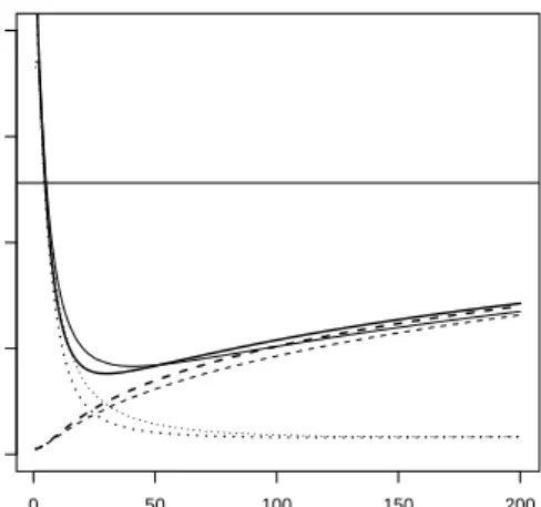
Figure 1 shows the (empirical) bias and variance for example data generated from model (3) which will be introduced in detail in Section 5. The minimum MSE obtainable is slightly smaller for boosted ridge regression, probably resulting from a faster drop-off of the bias component. We found this pattern prevailing in other simulated data examples, but the difference between boosted ridge regression and simple ridge regression usually is not large. Overall the fits obtainable from ridge regression and boosted ridge regression with the penalty parameter and the number of steps chosen appropriately are rather similar.
3
Partial and componentwise boosting
Simple boosted regression as considered in Section 2 yields estimates in cases where the ordinary least-squares estimator does not exist. However, as will be shown, in
particu-0 50 100 150 200 0.0 0.2 0.4 0.6 0.8 step no. bias/variance/MSE
Figure 1: Empirical bias and variance of ridge regression (thin lines) and boosted ridge regression (thick lines) (MSE: solid lines; bias: dotted lines; variance: broken lines) for example data
generated from (3) (see Section 5) with n= 100, p= 50, ρb = 0.7 and signal-to-noise ratio 1.
The horizontal scale of the ridge regression curves is adjusted to have approximately the same degrees of freedom as boosted ridge regression in each step.
lar for high dimensional predictor space the performance can be strongly improved by
updating only one component of β in one iteration. B¨uhlmann and Yu (2003) refer
to the method as componentwise boosting and propose to choose the component to be updated with reference to the resulting improvement of the fit. This powerful procedure implicitly selects variables to be included in the predictor. What comes as an advantage may turn into a drawback when covariates which are important to the practioner are not included. For example in case-control studies the variables may often be grouped into variables that have to be evaluated, including the treatment, and variables for which inclusion is optional, depending on their effect. Moreover, componentwise boosting does not distinguish between continuous and categorical predictors. In our studies continu-ous predictors have been preferred in the selection process, probably since continucontinu-ous predictors contain more information than binary variables.
par-tial boosting means that in one iteration selected components of the parameter vector
βT
(m) = (β(m),1, . . . , β(m),p) are re-estimated. The selection is determined by a specific
structuring of the parameters (variables). Let the parameter indices V ={1, . . . , p} be
partitioned into disjunct sets byV =Vc∪Vo1∪. . .∪VoqwhereVc stands for the
(compul-sory) parameters (variables) that have to be included in the analysis, and Vo1, . . . , Voq
represent blocks of parameters that are optional. A block Vor may refer to all the
parameters which refer to a multicategorical variable, such that not only parameters but variables are evaluated. Candidates in the refitting process are all combinations
Vc ∪Vor, r = 1, . . . , q, representing combinations of necessary and optional variables.
Componentwise boosting, as considered by B¨uhlmann and Yu (2003) is the special case
where in each iteration one component from β(m), say β(m),j, is reestimated, meaning
that the structuring is specified byVc =∅, Voj ={j}.
Let now Vm = (m1, . . . , ml) denote the indices of parameters to be considered for
refitting in the mth step. One obtains the actual design matrix from the full design
matrix X= (x·1, . . . , x·p) by selecting the corresponding columns, obtaining the design
matrix XVm = (x·m1, . . . , x·ml). Then in iteration m ridge regression is applied to the
reduced model yi−µˆ(m−1),i= (xi,m1, . . . , xi,ml) TβR Vm+εi yielding solutions ˆ βVRm = ( ˆβVRm,m1, . . . ,βˆRVm,ml) = (XT VmXVm+λIp) −1XT Vm(y−µˆ(m−1)).
The total parameter update is obtained from components
ˆ β(RVm),j= ˆ βVR m,j j∈Vm 0 j /∈Vm , yielding ˆβR(V m) = ( ˆβ R (Vm),1, . . . , ˆ βR(V m),p)
T. The corresponding update of the mean is given
by ˆµ(m) = ˆµ(m−1) +XVmβˆ
R
Vm = X( ˆβ(m−1)+ ˆβ
R
(Vm)), and the new parameter vector is
ˆ
In the general case where in themth step several candidate setsVm(j)= (m1(j), . . . , m(lj)),
j= 1, . . . , l, are evaluated, an additional selection step is needed. In summary themth
iteration step has the following form:
Iteration (mth step): PartBoostR
(a) Compute for j = 1, . . . , s, the parameter updates ˆβ(V(j)
m ), and the corresponding
means ˆ µ((jm))= ˆµ(m−1)+XV(j) m ˆ βV(j) m .
(b) Determine which ˆµ((jm)),j= 1, . . . , l improves the fit maximally.
With Vm denoting the subset which is selected in the mth step one obtains the
updates ˆβ(m) = ˆβ(m−1) + ˆβR(Vm), ˆµ(m) = X ˆ β(m). With S0 = X(XTX +λIp)−1XT, Sm =XVm(X T VmXVm+λIp) −1XT
Vm,m= 1,2, . . . the iterations are represented as
ˆ µ(m)= ˆµ(m−1)+Sm(y−µˆ(m−1)) and therefore ˆ µ(m)=Hmy whereHm=Pmj=0SjQij=1−1(I −Si).
IfSj =S,Hmsimplifies to the form of simple ridge boosting. One obtainscov(ˆµ(m)) =
σ2Hm2,bias= (Hm−I)µ, and the MSE has the form
M SE = 1
n(trace(σ
2H2
m) +µT(Hm−I)2µ).
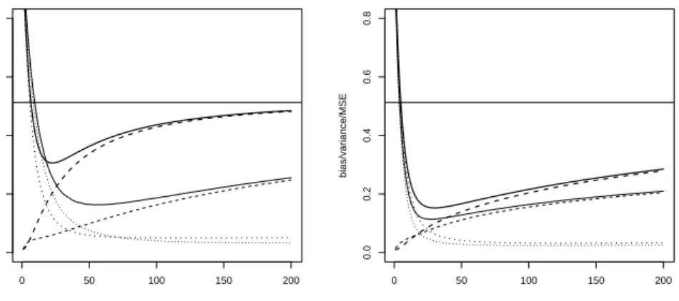
While mean squared error (MSE), bias and variance are similar for boosted ridge regression and simple ridge regression (Figure 1), differences can be expected when these approaches are compared to componentwise boosted ridge regression. Figure 2 shows MSE (solid lines), bias (dottes lines) and variance (broken lines) for the same data underlying Figure 1, this time for boosted ridge regression (thick lines) and the componentwise approach (thin lines). Penalties for both procedures have been chosen such that the bias curves are close in the initial steps. The fit of a linear model that
0 50 100 150 200 0.0 0.2 0.4 0.6 0.8 step no. bias/variance/MSE 0 50 100 150 200 0.0 0.2 0.4 0.6 0.8 step no. bias/variance/MSE
Figure 2: Empirical bias and variance of boosted ridge regression (thick lines) and componentwise boosted ridge regression (thin lines) (MSE: solid lines; bias: dotted lines; variance: broken lines)
for example data generated from (3) withn= 100,p= 50 and uncorrelated (ρb= 0) (left panel)
and correlated (ρb = 0.7) (right panel) covariates.
incorporates all variables is indicated by a horizontal line. In the left panel of Figure 2 there are five covariates (of 50 covariates in total) with true parameters unequal to zero and the correlation between all covariates is zero. It is seen that for data with a small number of uncorrelated informative covariates the componentwise approach results in a much smaller minimum MSE, probably due to a much slower increase of variance. When correlation among all covariates (i.e. also between the covariates with non-zero param-eters and the covariates with true paramparam-eters equal to zero) increases, the performance of boosted ridge regression comes closer to the componentwise approach (right panel of Figure 2). This may be due to the coefficient build-up scheme of BoostR (illustrated in Figure 3) that assigns non-zero parameters to all covariates.
The idea of a stepwise approach to regression where in each step just one predictor is updated is also found in stagewise regression (see e.g. Efron et al., 2004). The main difference is the selection criterion and the update: The selection criterion in stagewise regression is the correlation between each variable and the current residual and the
with one predictor is fitted for each variable and any model selection criterion may be used. Since stagewise regression is closely related to the Lasso and Least Angle Regression (Efron et al., 2004), it can be expected that componentwise boosted ridge regression is also similar to the latter procedures.
3.1 Example: Prostate Cancer
We applied componentwise boosted ridge regression and boosted ridge regression to the prostate cancer data used by Tibshirani (1996) for illustration of the Lasso. The data
with n = 97 observations come from a study by Stamney et al. (1989) that examined
the correlation between the (log-)level of prostate specific antigen and eight clinical mea-sures (standardized before model fit): log(cancer volume) (lcavol), log(prostate weight) (lweight), age, log(benign prostatic hyperplasia amount) (lbph), seminal vesical invasion (svi), log(capsular penetration) (lcp), Gleason score (gleason) and percentage Gleason scores 4 or 5 (pgg45).
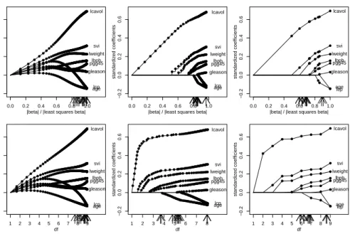
Figure 3 shows the coefficient build-up in the course of the boosting steps for two
scalings. In the top panels the values on the abscissa indicate theL2-norm of parameter
vector relative to the least-squares estimate, whereas in the bottom panels the degrees of freedom are given. A dot on the line corresponding to a coefficient indicates an estimate; thus each dot represents one step in the algorithm. While for boosted ridge regression (left panels) each coefficient seems to increase by a small amount in each step, in the componentwise approach (center panels) only to a specific set of variables non-zero coefficients are assigned within one step, the other coefficients remain zero. Therefore the coefficient build-up of the componentwise approach looks much more similar to that of the Lasso procedure (right panels) (fitted by the LARS procedure, see Efron et al., 2004). One important difference to the Lasso that can be seen in this example is that for BoostPartR the size of the coefficient updates varies over boosting steps in a specific pattern, with larger changes in the early steps and only small adjustments in late steps. Arrows indicate 10-fold cross-validation based on mean squared error which has been repeated over 10 distinct splittings to show variability. It is seen that cross-validation
−0.2
0.0
0.2
0.4
0.6
|beta| / |least squares beta|
standardized coefficients 0.0 0.2 0.4 0.6 0.8 1.0 lcavol lweight age lbph svi lcp gleason pgg45 ● ● ● ● ●● ●● ●●●●● ●●●● ●●●●●●●●●●●●●●●●●●●●●●●●●●●●●●●●●●●●●●●●●●●●●●●●●●●●●●●●●●●●●●●●●●●●●●●●●●●●●●●●●●●●●●●●●●●●●●●●●●●●●●●●●●●●●●●●●●●●●●●●●●●●●●●●●●●●●●●●●●●●●●●●●●●●●●●●●●●●●●●●●●●●●●●●●●●●●●●●●●●●●●● ● ● ●●● ● ●●●●● ●●●●●●●●●●●●●●●●●●●●●●●●●●●●●●●●●●●●●●●●●●●●●●●●●●●●●●●●●●●●●●●●●●●●●●●●●●●●●●●●●●●●●●●●●●●●●●●●●●●●●●●●●●●●●●●●●●●●●●●●●●●●●●●●●●●●●●●●●●●●●●●●●●●●●●●●●●●●●●●●●●●●●●●●●●●●●●●●●●●●●●●●●●●●● ● ●● ● ● ●●●●● ●●●●●●●●●●●●●●●●●●●●●●●●●●●●●●●●●●●●●●●●●●●●●●●●●●●●●●●●●●●●●●●●●●●●●●●●●●●●●●●●●●●●●●●●●●●●●●●●●●●●●●●●●●●●●●●●●●●●●●●●●●●●●●●●●●●●●●●●●●●●●●●●●●●●●●●●●●●●●●●●●●●●●●●●●●●●●●●●●●●●●●●●●●●●●● ● ●● ●● ●● ●●●●●●●●●●●●●●●●●●●●●●●●●●●●●●●●●●●●●●●●●●●●●●●●●●●●●●●●●●●●●●●●●●●●●●●●●●●●●●●●●●●●●●●●●●●●●●●●●●●●●●●●●●●●●●●●●●●●●●●●●●●●●●●●●●●●●●●●●●●●●●●●●●●●●●●●●●●●●●●●●●●●●●●●●●●●●●●●●●●●●●●●●●●●●●●●● ● ●● ●● ● ●●●●●●●●●●●●●●●●●●●●●●●●●●●●●●●●●●●●●●●●●●●●●●●●●●●●●●●●●●●●●●●●●●●●●●●●●●●●●●●●●●●●●●●●●●●●●●●●●●●●●●●●●●●●●●●●●●●●●●●●●●●●●●●●●●●●●●●●●●●●●●●●●●●●●●●●●●●●●●●●●●●●●●●●●●●●●●●●●●●●●●●●●●●●●●●●●● ● ● ●● ●●●●●●●●●●●●●●●●●●●●●●●●●●●●●●●●●●●●●●●●●●●●●●●●●●●●●●●●●●●●●●●●●●●●●●●●●●●●●●●●●●●●●●●●●●●●●●●●●●●●●●●●●●●●●●●●●●●●●●●●●●●●●●●●●●●●●●●●●●●●●●●●●●●●●●●●●●●●●●●●●●●●●●●●●●●●●●●●●●●●●●●●●●●●●●●●●●●● ● ●● ● ●●●●●●●●●●●●●●●●●●●●●●●●●●●●●●●●●●●●●●●●●●●●●●●●●●●●●●●●●●●●●●●●●●●●●●●●●●●●●●●●●●●●●●●●●●●●●●●●●●●●●●●●●●●●●●●●●●●●●●●●●●●●●●●●●●●●●●●●●●●●●●●●●●●●●●●●●●●●●●●●●●●●●●●●●●●●●●●●●●●●●●●●●●●●●●●●●●●● ● ● ● ●● ●●●●●●●●●●●●●●●●●●●●●●●●●●●●●●●●●●●●●●●●●●●●●●●●●●●●●●●●●●●●●●●●●●●●●●●●●●●●●●●●●●●●●●●●●●●●●●●●●●●●●●●●●●●●●●●●●●●●●●●●●●●●●●●●●●●●●●●●●●●●●●●●●●●●●●●●●●●●●●●●●●●●●●●●●●●●●●●●●●●●●●●●●●●●●●●●●●● −0.2 0.0 0.2 0.4 0.6
|beta| / |least squares beta|
standardized coefficients 0.0 0.2 0.4 0.6 0.8 1.0 lcavol lweight age lbph svi lcp gleason pgg45 ● ● ● ● ● ● ● ● ●● ●● ●●●●● ●●●●●●●●●●●●●●●●●●●●●●●●●●●●●●●●●●●●●●●●●●●●●●●●●●●●●●●●● ●● ●● ●●●● ●●●●●●●●●●●●●●●●●●●●●●●●●●●●●● ●●●●●●●●●●●●●●●●●●●●●●●●●●●●●●●●●●●●●●●●●●●●●●●●●●●●●●●●●●●●●●●●●●●●●●●●●●● ● ●●●●● ● ●●●●●●●●●●●●●●●●●●●●●●●●●●●●●●●●●●●●●●●●● ●● ●● ●●●● ●●●●●●●●● ● ●●●●●●●●●●●●●●●●●●●●●●●●●●●●●●●●●●●●●●●●●●●●●●●●●●● ● ● ●●●●●●●●●●●●●●●●●●●●●●●●●●●●●●●●●●●●●●●●●●●●●●●●●●●●●●●●●●●●●●●●●●●●●●●●●●●●●●●●●●●●●●●●●●●●●●●●●●●●●●●●●●●●●●●●●●● ● ● ●●●●●●●●●●●●●●●●●●●● ●●●●● ● ●●●●●●●●●●●●●●●●●●●●●●●●●●●●●●●●●●●●●●●●●●●●●●●●●●● −0.2 0.0 0.2 0.4 0.6
|beta| / |least squares beta|
standardized coefficients 0.0 0.2 0.4 0.6 0.8 1.0 lcavol lweight age lbph svi lcp gleason pgg45 ● ● ● ●● ● ● ● ● ● ●●● ● ● ● ● ● ● ●● ● ● ● ● ● ●● ● ● ● ● ●●● ● −0.2 0.0 0.2 0.4 0.6 df standardized coefficients 1 2 3 4 5 6 7 8 9 lcavol lweight age lbph svi lcp gleason pgg45 ● ● ● ●● ●● ●●●● ●●●● ●●●●●●●●● ●●●●●●●●●●●●●●●●●●●●●●●●●●●●●●●●●●●●●●●●●●●●●●●●●●●●●●●●●●●●●●●●●●●●●●●●●●●●●●●●●●●●●●●●●●●●●●●●●●●●●●●●●●●●●●●●●●●●●●●●●●●●●●●●●●●●●●●●●●●●●●●●●●●●●●●●●●●●●●●●●●●●●●●●●●●●●●●● ●● ●● ● ●●● ●●●●●●● ●●●●●●●●●●●●●●●●●●●●●●●●●●●●●●●●●●●●●●●●●●●●●●●●●●●●●●●●●●●●●●●●●●●●●●●●●●●●●●●●●●●●●●●●●●●●●●●●●●●●●●●●●●●●●●●●●●●●●●●●●●●●●●●●●●●●●●●●●●●●●●●●●●●●●●●●●●●●●●●●●●●●●●●●●●●●●●●●●●●●●●●●● ●● ● ● ● ● ●●●●●●●●●●● ●●●●●●●●●●●●●●●●●●●●●●●●●●●●●●●●●●●●●●●●●●●●●●●●●●●●●●●●●●●●●●●●●●●●●●●●●●●●●●●●●●●●●●●●●●●●●●●●●●●●●●●●●●●●●●●●●●●●●●●●●●●●●●●●●●●●●●●●●●●●●●●●●●●●●●●●●●●●●●●●●●●●●●●●●●●●●●●●●●●●●●● ●● ●● ● ● ●●●●●●●●●●●●●●●●●●●●●●●●●●●●●●●●●●●●●●●●●●●●●●●●●●●●●●●●●●●●●●●●●●●●●●●●●●●●●●●●●●●●●●●●●●●●●●●●●●●●●●●●●●●●●●●●●●●●●●●●●●●●●●●●●●●●●●●●●●●●●●●●●●●●●●●●●●●●●●●●●●●●●●●●●●●●●●●●●●●●●●●●●●●●●●●●●● ● ●● ●● ● ●●●●● ●●●●●●●●●●●●●●●●●●●●●●●●●●●●●●●●●●●●●●●●●●●●●●●●●●●●●●●●●●●●●●●●●●●●●●●●●●●●●●●●●●●●●●●●●●●●●●●●●●●●●●●●●●●●●●●●●●●●●●●●●●●●●●●●●●●●●●●●●●●●●●●●●●●●●●●●●●●●●●●●●●●●●●●●●●●●●●●●●●●●●●●●●●●●● ● ●● ● ●● ●●●●●●●●●●●●●●●●●●●●●●●●●●●●●●●●●●●●●●●●●●●●●●●●●●●●●●●●●●●●●●●●●●●●●●●●●●●●●●●●●●●●●●●●●●●●●●●●●●●●●●●●●●●●●●●●●●●●●●●●●●●●●●●●●●●●●●●●●●●●●●●●●●●●●●●●●●●●●●●●●●●●●●●●●●●●●●●●●●●●●●●●●●●●●●●●●● ●● ●● ● ● ●●●●●●●●●●●●●●●●●●●●●●●●●●●●●●●●●●●●●●●●●●●●●●●●●●●●●●●●●●●●●●●●●●●●●●●●●●●●●●●●●●●●●●●●●●●●●●●●●●●●●●●●●●●●●●●●●●●●●●●●●●●●●●●●●●●●●●●●●●●●●●●●●●●●●●●●●●●●●●●●●●●●●●●●●●●●●●●●●●●●●●●●●●●●●●●●●● ●● ●● ● ● ●●●●●●●●●●●●●●●●●●●●●●●●●●●●●●●●●●●●●●●●●●●●●●●●●●●●●●●●●●●●●●●●●●●●●●●●●● ●●●●●●●●●●●●●●●●●●●●●●●●●●●●●●●●●●●●●●●●●●●●●●●●●●●●●●●●●●●●●●●●●●●●●●●●●●●●●●●●●●●●●●●●●●●●●●●●●●●●●●●●●●●●●●●●●●●●●●●● −0.2 0.0 0.2 0.4 0.6 df standardized coefficients 1 2 3 4 5 6 7 8 lcavol lweight age lbph svi lcp gleason pgg45 ● ● ● ● ● ● ● ●● ●● ●●● ● ●●● ● ●●●●●●●●●●●● ●●●●●●●●●●●●●●●●●●●●●●●●●●●●●●●●●●●●●●●●●●● ●● ●●●●● ● ●●●● ● ●●●●●●●●● ●●●●●●●●●●●●●●●● ●●●●●●●●●●●●●●●●●●●●●●●●●●●●●●●●●●●●●●●●●●●● ●●●●●●●●●●●●●●●●●●●●●●●●●●●●●●● ●●●● ●●●●●●● ●●●●●●●●●●●●●●●●●●●●●●●●●●●●●●●●●●●●● ●● ●● ●●●● ● ●●●●●● ● ● ●●●●●●●●●●●●●●●●●●●●●●●●●●●●●●●●●●●●●●●●●●●●●●●●●●●● ●●●●●●●●●●●●●●●●●●●●●●●●●●●●●●●●●●●●●●●●●●●●●●●●●●●●●●●●●●●●●●●●●●●●●●●●●●●●●●●●●●●●●●●●●●●●●●●●●●●●●●●●●●●●●●●●●●●●● ●●●●● ● ●●●●●●●●●●●●●●●● ● ●●●● ● ●●●●●● ●●●●●●●●●●●●●●●●●●●●●●●●●●●●●●●●●●●●●●●●●●●●● −0.2 0.0 0.2 0.4 0.6 df standardized coefficients 1 2 3 4 5 6 7 8 9 lcavol lweight age lbph svi lcp gleason pgg45 ● ● ● ● ● ● ● ● ● ● ● ● ● ● ● ● ● ● ● ● ● ● ● ● ● ● ● ● ● ● ● ● ● ● ● ●
Figure 3: Coefficient build-up of BoostR (left panels), PartBoostR (center panels) and the Lasso
(right panels) for the prostate cancer data plotted against standardizedL2-norm of the parameter
vector (top panels) and degrees of freedom (bottom panels). Arrows indicate the model chosen by 10-fold cross-validation (repeated for 10 times).
selects a model of rather high complexity for boosted ridge regression. When using the componentwise approach or the Lasso, more parsimonious models are selected. Partial boosting selects even more parsimonious models than the Lasso in terms of degrees of freedom.
4
Ridge boosting in generalized linear models
In generalized linear models the dominating estimation approach is maximum likelihood
which corresponds to the use of L2 loss in the special case of normally distributed
responses. Ridge regression in generalized linear models is therefore based an penalized maximum likelihood. Univariate generalized linear models are given by
whereµi=E(yi|xi),his a given (strictly monotone) response function, and the predictor
ηi =zTi β has linear form. Moreover, it is assumed thatyi|xi is from the simple
exponen-tial family, including for example binary responses, Poisson distributed responses and gamma distributed responses.
The basic concept in ridge regression is to maximize the penalized log-likelihood
lp(β) = n X i=1 li− λ 2 p X i=1 βi2 = n X i=1 li− λ 2 p X i=1 βTP β
where li is the likelihood contribution of the ith observation and P is a block diagonal
matrix with the (1×1) block 0 and the (p×p) block given by the identy matrixIp. The
correspondingpenalized score function is given by
sp(β) = n X i=1 zi ∂h(ηi)/∂η σ2 i (yi−µi)−λP β. whereσ2
i =var(yi). A simple way of computing the estimator is iterative Fisher scoring
ˆ
β(k+1) = ˆβ(k)+Fp( ˆβ(k))−1sp( ˆβ(k)),
where Fp(β) = E(−∂l/∂β∂βT) = F(β) + λP, with F(β) denoting the usual Fisher
matrix given by F(β) = XTW(η)X, X = (x·0, x·1, . . . , x·p), xT·0 = (1, . . . ,1), W(η) =
D(η)Σ(η)−1D(η), Σ(η) = (σ21, . . . , σn2),D(η) =diag(∂h(η1)/∂η, . . . , ∂h(ηn)/∂η).
The proposed boosting procedure is likelihood based ridge boosting based on one step of Fisher scoring (for likelihood based boosting see also Tutz and Binder, 2004). The parameter/variable set to be refitted in one iteration now includes the intercept.
Let again Vm(j) denote subsets of indices of parameters to be considered for refitting in
themth step. Then Vm(j)={m1, . . . , ml} ⊂ {0,1, . . . , p}, where 0 denotes the intercept.
The general algorithm, including a selection step, is given in the following. In order
to keep the presentation simple the matrix formµ=h(η) is used whereµand η denote
Algorithm: GenBoostR
Step 1: Initialization
Fit model µi =h(β0) by iterative Fisher scoring obtaining ˆβ(0) = ( ˆβ0,0, . . . ,0), ˆη(0) =
Xβˆ(0)
Step 2: Iteration
Form= 1,2, . . .
(a) Estimation
Estimation for candidate setsVm(j) corresponds to fitting of the model
µ=h(ˆη(m−1)+XV(j) m β R Vm(j) ) where ˆη(m−1) = Xβˆ(m−1) and XVT(j) m = (x
im(j)1 , . . . , xim(j)l ) contains only
compo-nents from Vm(j).
One step of Fisher scoring is given by ˆ βR Vm(j) =F −1 p,Vm(j) sp,V(j) m where sp,V(j) m = XVm(j)W(ˆη(m−1))D −1(η (m−1))(y −µ(m−1)) (without −λP β = 0), F p,Vm(j) = X T Vm(j) W(ˆη(m−1))XV(j) m , with ˆη T (m−1) = (ˆη1,(m−1), . . . ,ηˆn,(m−1)), y T = (y1, . . . , yn), µT(m−1) = (µ1,(m−1), . . . , µn,(m−1)). (b) Selection
For candidate sets Vm(j), j = 1, . . . , s, the set Vm is selected that improves the fit
maximally. (c) Update One sets ˆ β(Rm)= ˆ βVRm,j j∈Vm 0 j /∈Vm, ˆ β(m) = ˆβ(m+1)+ ˆβ(Rm), ˆ η(m)=Xβˆ(m)=Xβˆ(m+1)+Xβˆ(Rm), ˆ
Within a generalized linear model framework it is natural to use in the selection step
(b) the improvement in deviance. With Dev(ˆη) denoting the deviance given predictor
values ˆη one selects in themth stepVm such thatDev(η(j)) is minimal, whereDev(η(j))
uses predictor value ˆη(j)= ˆηm−1+XV(j)
m
ˆ
βR
Vm(j)
.
Also stopping criteria should be based on the deviance. One option is deviance based cross-validation, an alternative choice is the AIC criterion
AIC =Dev(ˆη(m)) + 2dfm
or the Bayesian information criterion
BIC =Dev(ˆη(m)) + logn·dfm
wheredfm represents the effective degrees of freedom which are given by the trace of the
hat matrix (see Hastie and Tibshirani, 1990). In the case of generalized linear models the hat matrix is not as straightforward as in the simple linear model. The following proposition gives an approximate hat matrix (for proof see Appendix).
Proposition 3. An approximate hat matrix for which µˆ(m)≈Hmy is given by
Hm = m X j=0 Mj j−1 Y i=0 (I−M0) where Mm = Σ1m/2Wm1/2XVm(X T VmWmXVm+λI) −1X VmW 1/2 m Σ−m1/2, Wm = W(ˆη(m−1)), Dm =D(ˆη(m−1))
The approximate hat matrix yields the AIC criterion AIC =Dev(ˆη(m)) + 2tr(Hm).
5
Empirical comparison
For the investigation of the properties of boosted ridge regression we use simulated data. This allows us the modify systematically the structure of the data fed into the algorithms and to observe how the results change.
We generate a covariate matrix X by drawing n observations from a p-dimensional
(i.e. columns of X) xj and xk being ρ
|j−k|
b . The true predictor η (and thereby the
corresponding expected value of the responseE(y|x) =µ=h(η), wherehis the identity
for a continuous response andh(η) = exp(η)/(1 + exp(η)) for binary responses) is formed
by
η=Xβtrue (3)
where the true parameter vectorβtrue=cstn·(β1, . . . , βp)T is determined by
βj ∼N(5,1) forj∈Vinf o, βj = 0 otherwise
with Vinf o ⊂ {1, . . . ,10} being the set (of size 5) of the randomly drawn indices of the
informative covariates. The constantcstn is chosen such that the signal-to-noise ratio for
the final responsey, drawn from a normal distributionN(µ,1) or a binomial distribution
B(µ,1),is equal to 1. The signal-to-noise-ratio is determined by
signal-to-noise ratio = Pn i=1(µi−µ¯)2 Pn i=1V ar(yi) where ¯µ= n1 Pn
i=1µi. For the examples presented here we used fixed sample sizen= 100
for the training data and a new sample of sizennew= 1000 for the evaluation of prediction
performance.
The following comparisons of performance and identification of influential covariates of (Gen)BoostR and (Gen)PartBoostR with other procedures have been done within the statistical environment R 2.1.0 (R Development Core Team, 2004). We used intercept-only (generalized) linear models, the (generalized) Lasso (package “lasso2” 1.2-0 — LARS as used in Section 3.1 is only available for continuous response data) and the “elastic net” procedure (Zou and Hastie, 2005) (package “elastic net” 1.02) for compar-ison. We evaluate performance for optimal values of the tuning parameters as well as for parameters chosen by tenfold cross-validation.
For the Lasso only one parameter (the upper bound on theL1-norm of the parameter
vector) has to be chosen. We use a line search, which has to be augmented in some examples because for certain values no solution exists. Zou and Hastie (2005) also note this as a downside of the classical Lasso. The elastic net procedure has two tuning
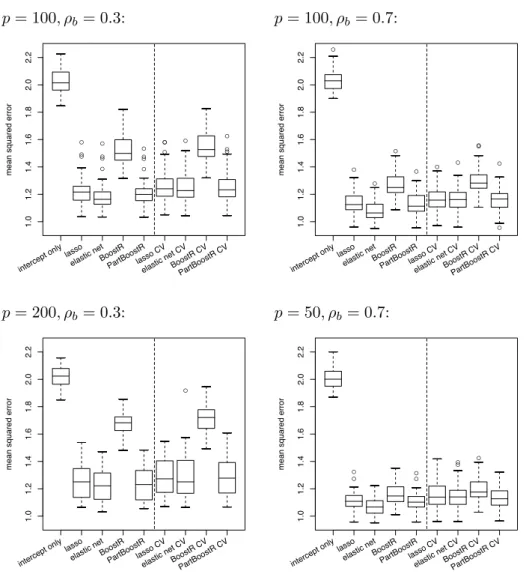
p= 100, ρb = 0.3: p= 100, ρb = 0.7: ● ● ● ● ● ● ● ● ● ● ● ● ● ● ● ● ● ● 1.0 1.2 1.4 1.6 1.8 2.0 2.2
mean squared error
intercept only lasso
elastic netBoostRPartBoostRlasso CV
elastic net CVBoostR CVPartBoostR CV
● ● ● ● ● ● ● ● ● ● ● 1.0 1.2 1.4 1.6 1.8 2.0 2.2
mean squared error
intercept only lasso
elastic netBoostRPartBoostRlasso CV
elastic net CVBoostR CVPartBoostR CV
p= 200, ρb = 0.3: p= 50, ρb = 0.7: ● 1.0 1.2 1.4 1.6 1.8 2.0 2.2
mean squared error
intercept only lasso
elastic netBoostRPartBoostRlasso CV
elastic net CVBoostR CVPartBoostR CV
● ● ● ● ● ● ● 1.0 1.2 1.4 1.6 1.8 2.0 2.2
mean squared error
intercept only lasso
elastic netBoostRPartBoostRlasso CV
elastic net CVBoostR CVPartBoostR CV
Figure 4: Mean squared error for continuous response data with varying number of predictorsp
and correlationρb for the linear model including only an intercept term, elastic net, the Lasso
BoostR and PartBoostR with tuning parameters selected for optimal performance or by cross-validation (CV).
parameters, the number of steps k and the penalty λ. We chose both by evaluating
a grid of steps 1, . . . , min(p, n) and penalties (0,0.01,0.1,1,10,100) (as suggested by
Zou and Hastie, 2005). For each of BoostR and PartBoostR we used a fixed penalty
parameterλ. This parameter has been chosen in advance such that the number of steps
5.1 Metric response
5.1.1 Prediction performance
The boxplots in Figure 4 show the mean squared error for continuous response data gen-erated from (3) with a varying number of predictors and amount of correlation between the covariates for 50 repetitions per example. In Figure 4 elastic net, the Lasso, boosted ridge regression and componentwise boosted ridge regression (with an intercept-only lin-ear model as a baseline) are compared for the optimal choice of tuning parameters (in the left part of the panels) as well for the cross-validation based estimates (in the right part).
When comparing the optimal performance of boosted ridge regression with the com-ponentwise approach, it is seen that the latter distinctly dominates the former for a large number of predictors (with only few of them being informative) (bottom left vs. top left panel) and/or small correlations (top left vs. top right panel). A similar difference in performance is also found when comparing boosted ridge regression to the Lasso and to the elastic net procedure. This highlights the similarity of the componentwise approach to the Lasso-type procedures (as illustrated in Section 3.1). When the close connection of BoostR and simple ridge regression is taken into consideration this replicates the results of Tibshirani (1996) who also found that in sparse scenarios the Lasso performs well and ridge regression performs poor. Consistently the performance difference for a smaller number of covariates and high correlation (bottom right panel) is less pronounced.
For optimal parameters no large differences between the performance of the compo-nentwise approach, the Lasso and of elastic net are seen. Elastic net seems to have a slightly better performance for examples with higher correlation among the predictors, but this is to be expected because elastic net was specifically developed for such high-correlation scenarios (see Zou and Hastie, 2005). The decrease in performance incurred by selecting the number of steps/Lasso constraint by cross-validation instead of using the optimal values is similar for componentwise boosted ridge regression and the Lasso. For the elastic net procedure the performance decrease is larger to such an extent that
the performance benefit over the former procedures (with optimal parameters) is lost. This might result from the very small range of the number of steps where good perfor-mance can be achieved (due to the small overall number of steps used by elastic net). In contrast boosting procedures change very slowly in the course of the iterative process, which makes selection of appropriate shrinkage more stable (compare Figure 3).
5.1.2 Identification of influential variables
While prediction performance is an important criterion for comparison of algorithms the variables included into the final model are also of interest. The final model should be as parsimonious as possible, but all relevant variables should be included. For example one of the objectives for the development of the elastic net procedure was to retain all important variables for the final model even when they are highly correlated (while the Lasso includes only some of a group of correlated variables; see Zou and Hastie, 2005).
The criteria by which the performance of a procedures in the identification of
influ-ential variables can be judged are thehit rate (i.e. the proportion of correctly identified
influential variables) hit rate = Pp 1 j=0I(βtrue,j 6= 0) p X j=1 I(βtrue,j6= 0)·I( ˆβj 6= 0)
and thefalse alarm rate (i.e. the proportion of non-influential variables dubbed
influen-tial)
false alarm rate = Pp 1
j=0I(βtrue,j = 0) p
X
j=1
I(βtrue,j= 0)·I( ˆβj 6= 0)
whereβtrue,j, j = 1, . . . , pare the elements of the true parameter vector, ˆβj are the
cor-responding estimates used by the final model andI(expression) is an indicator function
that takes the value 1 if “expression” is true and 0 otherwise.
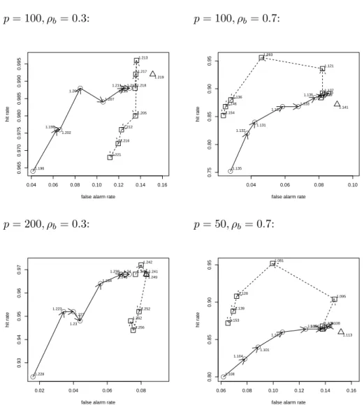
Figure 5 shows the hit rates and false alarm rates for componentwise boosted ridge regression (circles), elastic net (squares) and the Lasso (triangle) for the data underlying Figure 4. While the Lasso has only one parameter which is selected for optimal predic-tion performance, the componentwise approach and elastic net have two parameters, a
penalty parameter and the number of steps. For evaluation of prediction performance we used a fixed penalty for the componentwise approach and the optimal penalty (with respect to prediction performance) for the elastic net procedure. For the investigation of their properties with respect to identification of influential variables we vary the penalty parameters (the number of steps still being chosen for optimal performance), thus re-sulting in a sequence of fits. Plotting the hit rates and false alarm rates of these fits leads to the pseudo-ROC-curves shown in Figure 5. We call them “pseudo” curves since they are not necessarily monotone!
It is seen that for a large number of covariates and a medium level of correlation (bottom left panel) the componentwise approach comes close to dominating the other procedures. While for a smaller number of variables and medium level of correlation (top left panel) higher hit rates can be achieved by using the elastic net procedure the componentwise approach still is the only procedure which allows for a trade-off of hit rate and false alarm rate (and therefore selection of small false alarm rates) by variation of the penalty parameter. In this case for the elastic net the false alarm rate hardly changes.
For the examples with high correlations between covariates (right panels) there is a clear advantage for the elastic net procedure. With penalty parameters going toward zero elastic net comes close to a Lasso solution (as it should, based on its theory). This is also where the elastic net pseudo-ROC curve (for small penalties) and the curve of the componentwise approach (for large penalties) coincide. The differences seen between elastic net/componentwise solutions with small/large penalties and the Lasso solution might result from the different type of tuning parameter (number of steps vs. constraint on the parameter vector).
5.2 Binary response
In order to evaluate generalized boosted ridge regression and generalized component-wise boosted ridge regression for the non-metric response case we compare them to a generalized variant of the Lasso, which is obtained by using iteratively re-weighted least
p= 100, ρb = 0.3: p= 100, ρb = 0.7: ● ●● ● ● ●●● 0.04 0.06 0.08 0.10 0.12 0.14 0.16 0.965 0.970 0.975 0.980 0.985 0.990 0.995
false alarm rate
hit rate 1.196 1.198 1.202 1.204 1.207 1.211 1.213 1.216 1.219 1.218 1.217 1.213 1.205 1.212 1.216 1.221 ● ● ● ● ● ● ●● 0.04 0.06 0.08 0.10 0.75 0.80 0.85 0.90 0.95
false alarm rate
hit rate 1.135 1.132 1.131 1.131 1.133 1.135 1.1371.135 1.141 1.139 1.137 1.121 1.093 1.136 1.146 1.154 p= 200, ρb = 0.3: p= 50, ρb = 0.7: ● ● ● ● ● ● ● ● 0.02 0.04 0.06 0.08 0.93 0.94 0.95 0.96 0.97
false alarm rate
hit rate 1.228 1.223 1.227 1.23 1.234 1.238 1.24 1.243 1.249 1.245 1.242 1.241 1.252 1.256 1.262 ● ● ● ● ● ●●● 0.06 0.08 0.10 0.12 0.14 0.16 0.80 0.85 0.90 0.95
false alarm rate
hit rate 1.108 1.104 1.101 1.102 1.1051.106 1.108 1.109 1.113 1.11 1.108 1.095 1.081 1.128 1.139 1.153
Figure 5: Pseudo-ROC curves for the identification of influential and non-influential covariates with metric response data for PartBoostR (circles) and elastic net (squares) with varying penalty parameters (and the optimal number of steps) and for the Lasso (triangle). Arrows indicate increasing penalty parameters. The numbers give the mean squared error of prediction for the respective estimates.
squares with a pseudo-response where weighted least-squares estimation is replaced by a weighted Lasso estimate (see documentation of the “lasso2” package Lokhorst, 1999). The Lasso constraint parameter and the number of steps for (componentwise) boosted ridge regression are determined by cross-validation and we compare the resulting
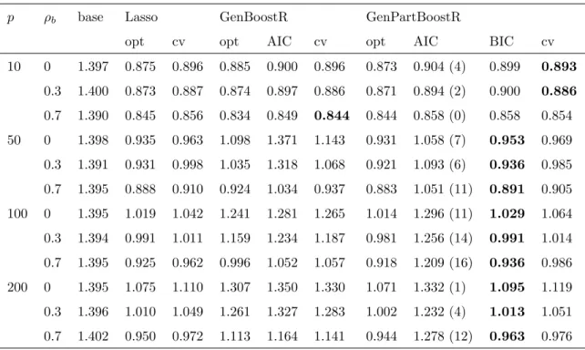
per-Table 1: Mean deviance (of prediction) for binary response data with varying number of
pre-dictors p and correlation ρb for a generalized linear model including only an intercept term
(base), generalized Lasso (with optimal constraint and constraint selected by cross-validation), generalized boosted ridge regression (GenBoostR) and generalized componentwise boosted ridge regression (GenPartBoostR) (with optimal number of steps and number of steps selected by AIC, BIC or cross-validation (cv)). The best result obtainable by data selected tuning parameters is marked in boldface for each example.
p ρb base Lasso GenBoostR GenPartBoostR
opt cv opt AIC cv opt AIC BIC cv
10 0 1.397 0.875 0.896 0.885 0.900 0.896 0.873 0.904 (4) 0.899 0.893 0.3 1.400 0.873 0.887 0.874 0.897 0.886 0.871 0.894 (2) 0.900 0.886 0.7 1.390 0.845 0.856 0.834 0.849 0.844 0.844 0.858 (0) 0.858 0.854 50 0 1.398 0.935 0.963 1.098 1.371 1.143 0.931 1.058 (7) 0.953 0.969 0.3 1.391 0.931 0.998 1.035 1.318 1.068 0.921 1.093 (6) 0.936 0.985 0.7 1.395 0.888 0.910 0.924 1.034 0.937 0.883 1.051 (11) 0.891 0.905 100 0 1.395 1.019 1.042 1.241 1.281 1.265 1.014 1.296 (11) 1.029 1.064 0.3 1.394 0.991 1.011 1.159 1.234 1.187 0.981 1.256 (14) 0.991 1.014 0.7 1.395 0.925 0.962 0.996 1.052 1.057 0.918 1.209 (16) 0.936 0.986 200 0 1.395 1.075 1.110 1.307 1.350 1.330 1.071 1.332 (1) 1.095 1.119 0.3 1.396 1.010 1.049 1.261 1.327 1.283 1.002 1.232 (4) 1.013 1.051 0.7 1.402 0.950 0.972 1.113 1.164 1.141 0.944 1.278 (12) 0.963 0.976
formance to that obtained with optimal parameter values. For the binary response
examples given in the following the AIC and the BIC (see Section 4) is available as an additional criterion for (componentwise) boosted ridge regression.
Table 1 gives the mean deviance for binary response data generated from (3) with
n= 100 and a varying number of variables and correlation for 20 repetitions per example.
When using the AIC as a stopping criterion in several instances (number indicated in parentheses) no minimum within the range of 500 boosting steps could be found and
so effectively the maximum number is used. It is seen that for a small number of
variables and high correlation between covariates (p = 10, ρb = 0.7)(generalized) ridge
regression and componentwise boosted ridge regression perform similar, for all other examples the componentwise approach is ahead. This parallels the findings from the continuous response examples. While it seems that there is a slight advantage of the componentwise approach over the Lasso, their performance (with optimal parameters as well as with parameters selected by cross-validation) is very similar. Selection of the number of boosting steps by AIC seems to work well only for a small number of variables, as can be seen e.g. when comparing to the cross-validation results for the componentwise approach. For a larger number of covariates the use of AIC for the selection of the number of boosting steps seems to be less efficient. In contrast BIC seems to perform quite well for a moderate to large number of covariates while being suboptimal for a smaller number of predictors.
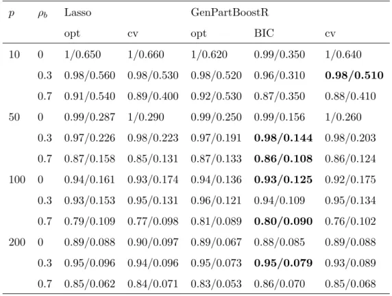
Table 2 shows the hit rates/false alarm rates obtained from the the componentwise approach and from the Lasso when using optimal parameters (number of boosting steps for GenPartBoostR and the constraint on the parameter vector for the Lasso) as well as for parameters chosen by cross-validation and BIC (for the componentwise approach). It is seen that with optimal parameters application of the componentwise approach can result in smaller false alarm rates compared to the Lasso while maintaining a competitive hit rate. This is similar to the continuous response examples and therefore the trade-off between hit rate and false alarm by selection of the penalty parameter seems to be feasible. Using BIC as a criterion for the selection of the number of boosting steps the combination of hit rate and false alarm rate obtained with componentwise boosted ridge regression even dominates the Lasso results in several instances (printed in boldface).
6
Application
We illustrate the application of (componentwise) boosted ridge regression with real data. The data are from 344 admissions at a psychiatric hospital with a specific diagnosis
Table 2: Hit rates/false alarm rates for identification of influential covariates with binary response data. Combinations of hit rate and false alarm rate obtained by cross-validation that dominate all other procedures for an example are printed in boldface.
p ρb Lasso GenPartBoostR
opt cv opt BIC cv
10 0 1/0.650 1/0.660 1/0.620 0.99/0.350 1/0.640 0.3 0.98/0.560 0.98/0.530 0.98/0.520 0.96/0.310 0.98/0.510 0.7 0.91/0.540 0.89/0.400 0.92/0.530 0.87/0.350 0.88/0.410 50 0 0.99/0.287 1/0.290 0.99/0.250 0.99/0.156 1/0.260 0.3 0.97/0.226 0.98/0.223 0.97/0.191 0.98/0.144 0.98/0.203 0.7 0.87/0.158 0.85/0.131 0.87/0.133 0.86/0.108 0.86/0.124 100 0 0.94/0.161 0.93/0.174 0.94/0.136 0.93/0.125 0.92/0.175 0.3 0.93/0.153 0.95/0.131 0.96/0.121 0.94/0.109 0.95/0.134 0.7 0.79/0.109 0.77/0.098 0.81/0.089 0.80/0.090 0.76/0.102 200 0 0.89/0.088 0.90/0.097 0.89/0.067 0.88/0.085 0.89/0.088 0.3 0.95/0.096 0.94/0.096 0.95/0.073 0.95/0.079 0.93/0.089 0.7 0.85/0.062 0.84/0.071 0.83/0.053 0.86/0.070 0.85/0.068
within a timeframe of eight years. The (binary) response variable to be investigated is whether treatment is aborted by the patient against physicians’ advice (about 55% for this diagnosis). There are five metric and 16 categorical variables from routine docu-mentation at admission available for prediction. This encompasses socio-demographic variables (age, sex, education, employment, etc.) as well as clinical information (level of functioning, suicidal behavior, medical history, etc.). After re-coding each categorical variable into several 0/1-variables for easier inclusion into a linear model there is a total of 101 predictors. The clinic’s interest is not primarily exact prediction but identifica-tion of informative variables that allow for an early intervenidentifica-tion to prevent patients with high risk from aborting treatment. Nevertheless we divide the data into 270 admissions
from the first six year interval for model building and the 74 admissions of the last two years for model validation. The baseline prediction error on the latter data using an intercept-only model is 0.446.
In a first step we apply componentwise boosted ridge regression and the Lasso with the full set of 101 predictors. From the physicians’ view one variable is of special interest and should be incorporated in the analysis. This is the secondary diagnosis assigned to the patient (taking either the value “none” or one of six diagnosis groups). For the Lasso we can either include the predictors coding for the secondary diagnosis without restriction or impose the same bound used for the other variables. We use the latter option, although this leads to estimates for only two of the secondary diagnosis groups, because the other predictors are excluded. With componentwise boosted ridge regression there is the option of making the secondary diagnosis predictors mandatory members of
the candidate setsVm(j), i.e. there will be estimates for them in any case. For a further
reduction of the complexity we use a special structure for the penalty matrix P with
larger penalty for the mandatory elements of the candidate sets. This option of using a customized penalization structure is another distinct feature of the componentwise approach in comparison to the Lasso.
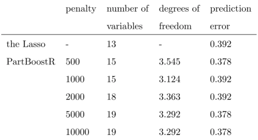
Table 3 shows the number of variables with non-zero parameter estimates, the ap-proximate degrees of freedom and the prediction error on the test data for the models resulting from componentwise boosted ridge regression with varying penalty parameter (with BIC) and the Lasso (with cross-validation). Note that the reason why the Lasso uses less variables compared to the componentwise approach is the use of the manda-tory parameters with the latter. It is seen that the performance of the componentwise approach is slightly superior to the Lasso. What is more interesting is that with varying penalty parameter the number of variables used for optimal performance also varies. This feature of the componentwise approach — using the penalty parameter to control the hit rate/false alarm rate (and thereby the number of variables in the model) while maintaining performance — has already been illustrated in Section 5, but it is assuring that it can also be found with real data. It should be noted that the number of
vari-Table 3: Number of variables with non-zero estimates, approximate degrees of freedom and prediction error on the test set for the binary response example with 101 predictors using com-ponentwise boosted ridge regression with various penalty parameters penalty and the Lasso. The number of boosting steps is selected by BIC and the Lasso bound is selected by cross-validation.
penalty number of degrees of prediction
variables freedom error
the Lasso - 13 - 0.392 PartBoostR 500 15 3.545 0.378 1000 15 3.124 0.392 2000 18 3.363 0.392 5000 19 3.292 0.378 10000 19 3.292 0.378
ables is not proportional to model complexity (represented by the approximate degrees of freedom). It seems that while the degrees of freedom approximately stay the same they are allocated to the covariates in a different way.
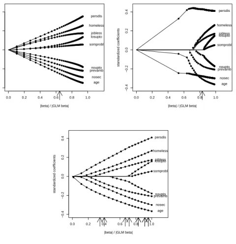
We already showed the coefficient build-up for a metric response example in Sec-tion 3.1. To obtain illustrative data for the binary response example we examine the predictors selected by the componentwise approach in the analysis above, combine sev-eral of those into new variables and add additional variables based on subject matter considerations. The variables used in the following are age, number of previous admis-sions (“noupto”), cumulative length of stay (“losupto”) and the 0/1-variables indicating a previous ambulatory treatment (“prevamb”), no second diagnosis (“nosec”), second diagnosis “personality disorder” (“persdis”), somatic problems (“somprobl”), homeless-ness (“homeless”) and joblesshomeless-ness (“jobless”). In contrast to the previous example with respect to the second diagnosis only the two most important group variables are used to keep the coefficient build-up graphs simple. Those two variables (“nosec” and “persdis”) again are mandatory members of the response set, but this time no penalty is applied to
−0.4 −0.2 0.0 0.2 0.4 |beta| / |GLM beta| standardized coefficients 0.0 0.2 0.4 0.6 0.8 1.0 nosec persdis noupto losupto age prevamb somprobl homeless jobless ● ● ● ● ● ● ●● ● ● ● ●●●● ●●●●● ●●●●●●●●●●●●●●●●●●●●●●●●●●●●●● ● ● ● ● ● ●● ●● ●● ●●● ●●●● ●●●●●●●●●●●●●●●●●●●●●●●●●●●●●●●● ● ● ● ● ● ● ●● ● ● ● ●●●●●●●●●●●●● ●●●●●●●●●●●●●●●●●●●●●●●●●● ● ● ● ● ●● ● ●● ● ● ●●●●●●●●●●● ●●●●●●●●●●●●●●●●●●●●●●●●●●●● ● ● ● ● ● ● ● ● ● ● ● ●●● ●●● ●●●●●●●●●●●●●●●●●●●●●●●●●●●●●●●●● ● ● ● ● ● ● ● ● ● ●● ●● ●●●●●● ●●●●●●●●●●●●●●●●●●●●●●●●●●●●●●● ● ● ● ● ●● ● ● ● ●● ●●●●●●●●●●●●●●●●●●●●●●●●●●●●●●●●●●●●●●● ● ● ● ● ● ●● ● ● ●● ● ●●●●●● ●●●●●●●●● ●●●●●●●●●●●●●●●●●●●●●●● ● ● ● ● ● ● ●● ● ● ● ●●●●●●●●●●●●●●● ●●●●●●●●●●●●●●●●●●●●●●●● −0.4 −0.2 0.0 0.2 0.4 |beta| / |GLM beta| standardized coefficients 0.0 0.2 0.4 0.6 0.8 1.0 nosec persdis noupto losupto age prevamb somprobl homeless jobless ● ●●●●●●●●●●●●●●●●●●●●●●●●●●●●●●●●●●●●●●●●●●●●●●●●●●●●●●●●●●●●●●●●●●●●●●●●●●●●●●●●●●●●●●●●●●●●●●●●●●●●●●●●●●●●●●●●●●●●●●●●●●●●●●●●●●●●●●●●●●●●●●●●●●●●●●●●●●●●●●●●●●●●●●●●●●●●●●●●●●●●●●●●●●●●●●●●●●●●●●●●●●●●●●●●●●●●●●●●●●●●●●●●●●●●●●●●●●●●●●●●●●●●●●●●●●●●●●●●●●●●●●●●●●●●●●●●●●●●●●●●●●●●●●●●●●●●●●●●●●● ● ●●●●●●●●●●●●●●●●●●●●●●●●●●●●●●●●●●●●●●●●●●●●●●●●●●●●●●●●●●●●●●●●●●●●●●●●●●●●●●●●●●●●●●●●●●●●●●●●●●●●●●●●●●●●●●●●●●●●●●●●●●●●●●●●●●●●●●●●●●●●●●●●●●●●●●●●●●●●●●●●●●●●●●●●●●●●●●●●●●●●●●●●●●●●●●●●●●●●●●●●●●●●●●●●●●●●●●●●●●●●●●●●●●●●●●●●●●●●●●●●●●●●●●●●●●●●●●●●●●●●●●●●●●●●●●●●●●●●●●●●●●●●●●●●●●●●●●●●●●● ●● ●● ●●●●●●●●●●●●●●●●●●●●●●●●●●●●●●●●●●●●●●●●●●●●●●●●●●●● ●●●●●●●●●●●●●●●●●●●●●●●●●●●●●●●●●●●●●●●●●●●●●●●●●●●●●●●●●●●●●●●●● ● ● ● ● ● ● ● ● ● ● ●● ●●●●●● ●●●●●●●●●●●●●●●●●●● ● ● ● ● ● ● ● ● ●●● ●●●●●●●●●●●●●● ●●●●●●●●●●●●●●●●●●●●●●● ●● ●● ● ●●● ●●● ●●●●●●●●●●●●●●●●●●●●●●●●●●●●●●●●●●●●●●●●●●●●●●●●● ●● ●● ●●●● ●●●●●●●●●●●●●●●●●●●●●●●●●● −0.4 −0.2 0.0 0.2 0.4 |beta| / |GLM beta| standardized coefficients 0.0 0.2 0.4 0.6 0.8 1.0 nosec persdis noupto losupto age prevamb somprobl homeless jobless ● ● ● ● ● ● ● ● ● ● ● ● ●● ● ● ● ●● ● ● ● ● ● ● ● ●● ● ●● ●●● ●● ●● ● ● ●● ● ● ● ● ● ● ● ● ● ●● ●● ●● ● ● ● ● ● ● ● ● ● ● ● ● ● ● ● ● ● ● ●● ● ● ● ● ● ● ● ● ● ● ● ● ●● ● ● ● ● ● ●● ● ● ●● ● ● ●● ● ● ●● ●● ●● ●●● ●● ● ●● ● ● ● ● ●●● ●● ● ● ●● ●
Figure 6: Coefficient build-up for example data (boosted ridge regression: upper left; componen-twise boosted ridge regression: upper right; the Lasso: bottom panel).
their estimates. This illustrates the effect of augmenting an unpenalized model with few mandatory variables with optional predictors. The top right panel of Figure 6 shows the coefficient build-up in the course of the boosting steps for componentwise boosted ridge regression contrasted with boosted ridge regression (top left) and the Lasso (bottom panel). The arrows indicate the number of steps chosen by AIC (for (componentwise) boosted ridge regression) and 10-fold cross-validation (for the Lasso; repeated for 10 times). It can be seen that while for the optional predictors the componentwise ap-proach results in a build-up scheme similar to the Lasso, the mandatory components