2017-13
Working paper. Economics
ISSN 2340-5031
Quantile Factor Models
/LDQJ&KHQ-XDQ-'RODGRDQG-HV~V*RQ]DOR
Serie disponible en http://hdl.handle.net/10016/11
Web: http://economia.uc3m.es/
Correo electrónico: [email protected]
Creative Commons Reconocimiento-NoComercial- SinObraDerivada 3.0 España
Quantile Factor Models
Liang Chen
1, Juan J. Dolado
2, and Jesús Gonzalo
31School of Economics, Shanghai University of Finance and Economics, [email protected] 2Department of Economics, Universidad Carlos III de Madrid, [email protected]
3Department of Economics, Universidad Carlos III de Madrid, [email protected]
April 20, 2019 Abstract
Quantile FactorModels (QFM) represent a new class of factor models for high-dimensional panel data. Unlike Approximate Factor Models (AFM), where only mean-shifting factors can be extracted, QFM also allow to recover unobserved factors shifting other relevant parts of the distributions of observed variables. A quantile regression approach, labeled Quantile Factor Analysis (QFA), is proposed to consistently estimate all the quantile-dependent factors and loadings. Their asymptotic distribution is then derived using a kernel-smoothed version of the QFA estimators. Two consistent model selection criteria, based on information criteria and rank minimization, are developed to determine the number of factors at each quantile. Moreover, in contrast to the conditions required for the use of Principal Components Analysis in AFM, QFA estimation remains valid even when the idiosyncratic errors have heavy-tailed distributions. Three empirical applications (regarding climate, financial and macroeconomic panel data) provide evidence that extra factors shifting quantiles other than the means could be relevant in practice.
Keywords: Factor models, quantile regression, incidental parameters. JEL codes: C31, C33, C38.
We are indebted to Ulrich Müller and four anonymous referees for their valuable comments and suggestions. We are also grateful
to Dante Amengual, Manuel Arellano, Steve Bond, Guillaume Carlier, Valentina Corradi, Jean-Pierre Florens, Alfred Galichon, Peter R. Hansen, Jerry Hausman, Sophocles Mavroeidis, Bent Nielsen, Enrique Sentana, Liangjun Su, and participants at several seminars and workshops for many helpful discussions. Financial support from the National Natural Science Foundation of China (Grant No.71703089), The Open Society Foundation, The Oxford Martin School, the Spanish Ministerio de Economía y Competitividad (grants ECO2016-78652 and Maria de Maeztu MDM 2014-0431), Bank of Spain (ER grant program), and MadEco-CM (grant S205/HUM-3444) is gratefully
1
Introduction
Following the key contributions byRoss(1976),Chamberlain and Rothschild (1983) and Con-nor and Korajczyk (1986) to the theory of approximate factor models (AFM henceforth) in the context of asset pricing, the analysis and applications of this class of models have prolif-erated thereafter. As is well known, AFM imply that a panel Xit of N variables (units), each with T observations, has a factor-structure representation given by: Xit = 0ift+✏it, where i = [ 1i, .., ri]0 and ft = [f1t, .., frt]0 are r⇥1 vectors of factor loadings and common factors, respectively, with r ⌧ N, and ✏it are zero-mean weakly dependent idiosyncratic disturbances which are uncorrelated with the factors.
The fact that it is easy to construct theories involving common factors, at least in a narrative version, together with the availability of simple estimation procedures for AFM — being Prin-cipal Components Analysis (PCA hereafter) the most popular, has led to their extensive use in many fields of economics.1 More recently, a conventional characterization of cross-sectional de-pendence among error terms in Panel Data has relied on the use of a finite number of unobserved common factors. These originate from economy-wide shocks that a↵ect all units with di↵erent intensities (loadings), in addition to idiosyncratic (individual-specific) disturbances. Interactive fixed-e↵ects models can be easily estimated by PCA (see Bai 2009) or by common correlated e↵ects (see Pesaran 2006), and there are even generalizations of these techniques dealing with nonlinear panel single-index models (see Chen et al. 2018). Likewise, the surge of Big Data technologies has made factor models a key tool in dimension reduction and predictive analytics for very large datasets (seeDiebold 2012 for a survey).
Our departure point in this paper is to notice that the standard regression interpretation of a static AFM as a linear conditional mean model of Xit given ft, that is, E(Xit|ft) = 0ift, entails two possibly restrictive features. First, PCA does not capture hidden factors that may shift characteristics (moments or quantiles) of the distribution of Xit other than the means. Second, neither the loadings i nor the factors ft are allowed to vary across the distributional characteristics of each unit in the panel.
A simple way of illustrating the limitations of the conventional formulation of AFM is to consider the factor structure in the following simple location-scale shift model: Xit = ↵if1t+
f2t✏it, with f1t 6= f2t (both are scalars), f2t > 0 and E(✏it) = 0, such that the first factor (f1t) shifts location, whereas the second one (f2t) shifts scale2. This model can be rewritten in quantile-regression (QR, hereafter) format as Xit = 0i(⌧)ft+uit(⌧), with 0< ⌧ < 1, i(⌧) = 1See,inter alia, Bai and Ng (2008b) andStock and Watson (2011). Early applications of AFM abound in
Aggregation Theory, Consumer Theory, Business Cycle Analysis, Finance, Monetary Economics, and Monitoring and Forecasting, among others.
2This model is further discussed in subsection 2.2 below, alongside other illustrative models representing
[↵i,Q✏(⌧)]0,ft= [f1t, f2t]0,uit(⌧) =f2t[✏it Q✏(⌧)], whereQ✏(⌧) represents the quantile function of✏it, and the conditional quantileQuit(⌧)[⌧|ft] = 0.
3 PCA will only extract the location-shifting factor f1t in this model, but it will fail to capture the scale-shifting factorf2t and the quantile-dependent loadings i(⌧) in its QR representation. Also notice that, when the distribution of ✏it is symmetric, then ft could be considered as being quantile dependent, i.e., ft(⌧), since
ft(⌧) = f1t for ⌧ = 0.5, and ft(⌧) = [f1t, f2t]0 for ⌧ 6= 0.5. Together with other examples discussed in subsection 2.2 further below, this means that the general class of models to be considered in the sequel would be one where the loadings, the factors and the number of factors are all simultaneously allowed to be quantile-dependent objects, namely, i(⌧), ft(⌧)2Rr(⌧) for ⌧ 2 (0,1). In what follows, we denote this class of models as Quantile Factor Models (QFM, hereafter), whose detailed definition is provided in Section 2 below.
That said, our goal in this paper is to develop a common factor methodology for QFM which is flexible enough to capture those quantile-dependent objects which standard AFM tools may be unable to recover. To do so, we analyze their estimation and inference, including the selection of the number of factors at each quantile ⌧. In a nutshell, QFM could be thought of as capturing the same type of flexible generalization that QR techniques represent for linear regression models.
To help understand how this new methodology works, we first propose an estimation ap-proach for the quantile-dependent objects in QFM, labeled Quantile Factor Analysis (QFA, henceforth). The QFA estimation procedure relies on the minimization of the standard check
function in QR (instead of the standard quadratic loss function used in AFM) to jointly esti-mate the common factorsft(⌧) and the loadings i(⌧) at a given quantile⌧.However, since the objective function for QFM is not convex in the relevant parameters, we introduce an iterative QR algorithm that yields estimators of the quantile-dependent objects. We then derive their average rates of convergence, and propose two consistent selection criteria, based on information criteria and rank minimization, to choose the number of factors at each ⌧. In addition, we establish asymptotic normality for QFA estimators based on smoothed QR (see e.g., Horowitz 1998 and Galvao and Kato 2016). Lastly, our asymptotic results and the proposed selection criteria provide guidance on how to discriminate between AFM and QFM structures.
The key contributions of our paper to the literature on FM can be summarized as follows: 1. We propose a new class of factor structures, QFM, provide an estimation method, QFA,
of the underlying quantile-dependents objects in QFM, and characterize the asymptotic properties of such estimators. In particular, we show that the average convergence rates of the QFA estimators are the same as the PCA estimators ofBai and Ng (2002), which is a crucial result for showing the consistency of the two selection criteria used to estimate the number of factors at each ⌧. In addition, similar to Bai (2003), our QFA estimators 3Throughout the paper we useQ
based on smoothed QR are shown to converge at the parametric rates (pN and pT) to normal distributions.
2. The problems of incidental parameters and non-smooth object functions require innovative strategies to derive all the above-mentioned results. This leads to the use in our proofs of some novel techniques borrowed from the theory of empirical processes. Moreover, our proof strategy can be easily extended to some other nonlinear factor models (e.g., probit and logit factor models considered by Chen et al. 2018) with smooth object functions. 3. The QFA estimators inherit from QR certain robustness properties to the presence of
outliers and heavy-tailed distributions in the idiosyncratic component of a factor model which render PCA invalid. In e↵ect, while PCA requires the idiosyncratic errors to have eighth bounded moments, QFA only needs the existence and smoothness of the density function. Thus, at⌧ = 0.5, QFA can be viewed as a robust alternative to PCA.
4. The extra factors obtained by the QFA estimation procedure can be used to improve the monitoring and forecasting performance of variables in a factor-augmented regression setup, as well as to facilitate the factor identification process, depending on the application at hand. For instance, in finance these “new” factors could be interpreted as volatility or tail-risk factors driving assets returns; with income data, they could represent common factors behind income inequality; and with climate data they could represent common features behind global extreme temperatures at both tails of their distribution, etc.
Related literature
There is a recent literature that attempts to make the AFM setup more flexible. For example, Su and Wang(2017) allow the factor loadings to be time varying, whilePelger and Xiong(2018) allow them to be state dependent. Chen et al. (2009) provide a theory for nonlinear principal components, where they suggest using sieve estimation to retrieve nonlinear factors. Finally, Gorodnichenko and Ng (2017) propose an algorithm to estimate level and volatility factors simultaneously. Di↵erent from these studies, our approach to modelling nonlinearities in factor models is through the conditional quantiles of the observed variables.
There is also a growing literature on heterogeneous panel quantile models with factor struc-tures, especially in financial economics. The main idea is that a few unobservable factors explain co-movements of asset return distributions in a large range of asset returns observed at high fre-quencies, as in stock markets. In parallel and independent research, we have recently come across two related studies to ours which focus on similar issues.4 First,Ma et al.(2017) propose estimation and inference procedures in semiparametric quantile factor models, in which factor loadings/betas are smooth functions of a small number of observables under the assumption that the included factors all have non zero mean. Then, sieve techniques are used to obtain 4We only became aware of these two papers after the working paper version of our study, referred to in the
preliminary estimation of these functions for each time period; next the factor structure is im-posed in a sequential fashion to estimate the factor returns by GLS under weak conditions on cross-sectional and temporal dependence. We depart from these authors in that we do not need to assume the loadings to depend on observables and, foremost, in that not only loadings but also factors are quantile-dependent objects in our setup.
Second, in a closely related paper, Ando and Bai (2018) (AB 2018, hereafter) use a setup similar to ours where the unobservable factor structure is also allowed to be quantile dependent. They use Bayesian MCMC and frequentist estimation approaches, the latter building upon our iterative procedure, as it is duly acknowledged in their paper. However, we di↵er from AB (2018) in several respects which could make our QFA approach valuable: (i) our assumptions are less restrictive, since we rely on properties of the density, as in QR, while AB (2018) needs all the moments of the idiosyncratic errors to exist, (ii) the proofs of the main results are also noticeably di↵erent since we believe that our proof strategy can solve some potential problems appearing in theirs, (iii) our rank-minimization selection criterion to estimate the number of factors is computationally more efficient and exhibits a better finite-sample performance than the information-criteria-based method considered by AB (2018).
Lastly, it is also worth highlighting that the illustrative location-scale shift model above, where f1t 6= f2t, is behind a current line of research in asset pricing which has been coined
the “idiosyncratic volatility puzzle” by Ang et al. (2006). This approach focuses on the co-movements in the idiosyncraticvolatilities of a panel of asset returns, and basically consists of applying PCA to the squared residuals, once the PCA mean-shifting factors have been removed from the data (a procedure labeled PCA-SQ, hereafter).5 For example, this technique would fit perfectly to the illustrative example discussed above. Yet, while the QFA estimation approach is able to recover the whole factor structure for more general models than the previous one (see subsection 2.2) or when the idiosyncratic errors lack bounded eighth moments, PCA-SQ fails to do so. Hence, to the best of our knowledge, QFA becomes the first estimation procedure capable of dealing with these issues.
Structure of the Paper. The rest of the paper is organized as follows. Section 2 defines QFM and provides a list of simple illustrative examples where the new QFM methodology applies. In Section 3, we present the QFA estimator and its computational algorithm, establish the average rates of convergence of all the quantile-dependent objects, and propose two consistent selection criteria to choose the number of factors at each quantile, which help when discriminating between AFM and QFM. Section 4 introduces a kernel-smoothed version of the QFA estimators to derive their asymptotic distributions. Section 5 contains some Monte Carlo simulation results to evaluate the performance in finite samples of our estimation procedures relative to other 5See, e.g.,Barigozzi and Hallin 2016,Herskovic et al. 2016andRenault et al. 2017. Notice that the volatility
co-movement does not arise from omitted factors in the AFM but from assuming a genuine factor structure in the idiosyncratic volatility processes.
alternative approaches under di↵erent assumptions about the idiosyncratic error terms. Section 6 considers several empirical applications using three large panel datasets, where we document the relevance of factors shifting other moments of the distributions of the data rather than just their means. Finally, Section 7 concludes and suggests several avenues for further research. Proofs of the main results are collected in the online appendix.
Notations: We use k·k to denote the Frobenius norm. For a matrix A with real eigenvalues, let ⇢j(A) denote the jth largest eigenvalue. Following Van der Vaart and Wellner (1996), the symbol.means “left side bounded by a positive constant times the right side” (the symbol& is defined similarly), andD(·, g,G) denotes the packing number of spaceG endowed with metric
g.
2
The Model and Some Examples
This section starts by introducing the main definitions to be used throughout the paper. Next, we show how to derive the QFM representation of several illustrative DGPs exhibiting di↵erent factor structures.
2.1 Quantile Factor Models
Suppose that the observed variableXit,withi= 1, .., N andt= 1, ..., T, has the following QFM structure:
Xit= 0i(⌧)ft(⌧) +uit(⌧), for ⌧ 2(0,1), (1) where the common factorsft(⌧) is ar(⌧)⇥1 vector of unobservable random variables, i(⌧) is ar(⌧)⇥1 vector of fixed factor loadings, and the idiosyncratic erroruit(⌧) is assumed to satisfy the following quantile restriction:
P[uit(⌧)0|ft(⌧)] =⌧.
Alternatively, (1) implies that
QXit[⌧|ft(⌧)] = 0i(⌧)ft(⌧),
where the factors, the loadings, and the number of factors are all allowed to be quantile-dependent.
2.2 Examples
In this section we provide a few illustrative examples of QFMs derived from di↵erent specifi-cations of location-scale shift models and related ones. By means of these simple illustrations, the objective is to show that there are instances where the standard AFM methodology fails to capture the full factor structure and therefore requires the use of our alternative QFM approach.
Example 1. Location-shift model. Xit =↵if1t+✏it, where {✏it} are zero-mean i.i.d errors
independent of f1t with cumulative distribution function (CDF) F✏. Let Q✏(⌧) = F✏1(⌧) =
inf{c : F✏(c) ⌧} be the quantile function of ✏it. Moreover, assume that the median of ✏it is
0, i.e., Q✏(0.5) = 0, then this simple model has a QFM representation (1) by defining i(⌧) =
[Q✏(⌧),↵i]0, ft(⌧) = [1, f1t]0 for ⌧ 6= 0.5, and i(⌧) =↵i, ft(⌧) =f1t for ⌧ = 0.5. However, note
that the standard estimation method (PCA) for this AFM may not be consistent if the distribution
of ✏it has heavy tails. For example, Assumption C of Bai and Ng (2002) requires E[✏8it] < 1,
which is not satisfied if, e.g. ✏it follows the standard Cauchy or some Pareto distributions .
Example 2. Location-scale shift model (same sign-restricted factor). Xit = ↵if1t+
f1t✏it, where f1t > 0 for all t and {✏it} are defined as in Example 1. This model has a QFM
representation (1) by defining i(⌧) =Q✏(⌧) +↵i andft(⌧) =f1tfor all⌧, such that the loadings
of the factor f1t are the only quantile-dependent objects.
Example 3. Location-scale shift model (di↵erent factors). Xit = ↵i0f1t+ (⌘0if2t)✏it,
where {✏it} are defined as in Example 1, ↵i, f1t 2Rr1, ⌘i, f2t 2Rr2, and ⌘i0f2t > 0, such that
fjt (j = 1,2) are vectors of rj factors. When f1t and f2t do not share common elements, this
model has a QFM representation (1) with i(⌧) = [↵i0,⌘i0Q✏(⌧)]0, ft(⌧) = [f10t, f20t]0 for ⌧ 6= 0.5, and i(⌧) =↵i, ft(⌧) =f1t for ⌧ = 0.5.
Example 4. Location-scale shift model with two idiosyncratic errors. Xit = ↵if1t+
f2t✏it+f3teit, where✏it and eit are two independent normal random variables with variances 2✏
and e2. This model is observationally equivalent toXit=↵if1t+
p
f22t 2
✏ +f32t 2e·vit where vit
follows a standard normal distribution. Thus, it has a QFM representation (1) with i(⌧) =
[↵i, 1(⌧)]0, ft(⌧) = [f1t, p
f2
2t ✏2+f32t e2]0 for ⌧ 6= 0.5, and i(⌧) =↵i, ft(⌧) =f1t for ⌧ = 0.5,
where 1 is the quantile function of the standard normal distribution.
Example 5. Location-scale shift model with an idiosyncratic error and its cube. Xit= ↵if1t+f2t✏it+cif3t✏3it, where✏itis a standard normal random variable. Letf2t, f3t, ci be positive,
then Xit has an equivalent representation in form of (1) with i(⌧) = [↵i, 1(⌧), ci 1(⌧)3]0,
ft(⌧) = [f1t, f2t, f3t]0 for ⌧ 6= 0.5, and i(⌧) = ↵i, ft(⌧) = f1t for ⌧ = 0.5. In particular, if
ci = 1 for alli and noticing that the mapping ⌧ 7! 1(⌧)3 is strictly increasing, then we have
for ⌧ 6= 0.5, QXit[⌧|ft(⌧)] = ↵if1t+
1(⌧)·[f
2t+f3t 1(⌧)2], so that there exists a QFM
Notice that in this case, the second factor in ft(⌧),f2t+f3t 1(⌧)2, is quantile dependent even
for ⌧ 6= 0.5.
Not surprisingly, PCA only works in Example 1, which corresponds to an AFM, when the idiosyncratic errors satisfy certain moment conditions. In all the remaining cases, PCA will only yield consistent estimates of the location-shift factors; however, it will fail to capture those extra factors which shift quantiles other than the means (Examples 3, 4 and 5) and, even if it extracts all relevant factors, it will miss their corresponding quantile-varying loadings (Example 2). In the sequel, we will therefore propose QFA as a new estimation procedure to estimate both sets of quantile-dependent objects in QFM.
3
Estimators and Their Asymptotic Properties
To simplify the notations, we suppress hereafter the dependence offt(⌧), i(⌧), r(⌧) and uit(⌧) on ⌧, so that the QFM in (1) is rewritten as:
Xit= 0ift+uit, P[uit0|ft] =⌧, (2)
where i, ft 2 Rr. Suppose that we have a sample of observations {Xit} generated by (2) for
i= 1, . . . , N,and t= 1, . . . , T, where the realized values of{ft}are{f0t}and the true values of { i} are { 0i}. We take a fixed-e↵ects approach by treating { 0i} and {f0t} as parameters to be estimated. In Section 3.1, we consider the estimation of { 0i} and {f0t} while r is assumed to be known. Section 3.2 deals with the estimation ofrfor each quantile. Finally, in Section 3.3 we discuss how to discriminate between AFM and QFM based the estimated number of mean and quantile factors.
3.1 Estimating Factors and Loadings
It is well known in the literature on factor models that { 0i} and {f0t} cannot be separately identified without imposing normalizations (see Bai and Ng 2002). Without loss of generality, we choose the following normalizations:
1 T T X t=1 ftft0 =Ir, 1 N N X i=1
i 0i is diagonal with non-increasing diagonal elements. (3)
Let M = (N +T)r, ✓ = ( 01, . . . , 0N, f10, . . . , fT0)0, and ✓0 = ( 001, . . . , 00N, f010 , . . . , f00T)0 denotes the vector of true parameters, where we also suppress the dependence of✓and ✓0 on M
to save notation. LetA,F ⇢Rr and define: ⇥M = ✓2RM :
i 2A, ft2F for all i, t,{ i}and {ft}satisfy the normalizations in (3) . Further, define: MN T(✓) = 1 N T N X i=1 T X t=1 ⇢⌧(Xit 0ift)
where⇢⌧(u) = (⌧ 1{u0})u is the check function. The QFA estimator of ✓0 is defined as:
ˆ
✓= (ˆ01, . . . ,ˆ0N,fˆ10, . . . ,fˆT0)0 = arg min ✓2⇥M MN T
(✓).
It is obvious that the way in which our estimator is related to the PCA estimator studied by Bai and Ng (2002) and Bai (2003) is analogous to how standard least-squares regressions are related to QR. However, unlikeBai (2003)’s PCA estimator, our estimator ˆ✓ does not yield an analytical closed form. This makes it difficult not only to find a computational algorithm that would yield the estimator, but also the analysis of its asymptotic properties. In the sequel, we introduce a computational algorithm called iterative quantile regression (IQR, hereafter) that can e↵ectively find the stationary points of the object function. In parallel, Theorem 1 shows that ˆ✓ achieves the same convergence rate as the PCA estimators for AFM.
To describe the algorithm, let ⇤= ( 1, . . . , N)0,F = (f1, . . . , fT)0, and define the following averages: Mi,T( , F) = 1 T T X t=1 ⇢⌧(Xit 0ft) and Mt,N(⇤, f) = 1 N N X i=1 ⇢⌧(Xit 0if).
Note that we have MN T(✓) = N 1PNi=1Mi,T( i, F) = T 1PTt=1Mt,N(⇤, ft). The main dif-ficulty in finding the global minimum of MN T is that this object function is not convex in ✓. However, for given F, Mi,T( , F) happens to be convex in for each i and likewise, for given ⇤, Mt,N(⇤, f) is convex in f for each t. Thus, both optimization problems can be efficiently solved by various linear programming methods (see Chapter 6 of Koenker 2005). Based on this observation, we propose the following iterative procedure:
Iterative quantile regression (IQR):
Step 1: Choose random starting parameters: F(0).
Step 2: Given F(l 1), choose (il 1) = arg min Mi,T( , F(l 1)) for i = 1, . . . , N; given ⇤(l 1), choose ft(l) = arg minfMt,N(⇤(l 1), f) for t= 1, . . . , T.
Step 3: Forl= 1, . . . , L, iterate the second step untilMN T(✓(L)) is close toMN T(✓(L 1)), where ✓(l)= (vech(⇤(l))0,vech(F(l))0)0.
To see the connection between the IQR algorithm and the PCA estimator proposed by Bai (2003), suppose that r = 1, and replace the check function in the IQR algorithm by the least-squares loss function. Then, it is easy to show that the second step of the algorithm above yields⇤(l 1)= (X0F(l 1))/kF(l 1)k2 and F(l)= (X⇤(l 1))/k⇤(l 1)k2 =XX0F(l 1)/Cl 1,
where X is the T ⇥N matrix with elements {Xit}, and Cl = kF(l)k2 ·k⇤(l)k2. Thus, the iterative procedure is equivalent to the well-known power method of Hotelling (1933); after normalizations, the sequenceF(0), F(1), . . . will converge to the eigenvector associated with the largest eigenvalue ofXX0, as in the PCA estimator ofBai(2003). Therefore, the IQR algorithm, and its corresponding QFA estimator, can be viewed as an extension of PCA to QFM using QR tools.
Similar algorithms have been proposed in the machine learning literature to reduce the dimensions for binary data, where the check function is replaced by some smooth nonlinear link functions, e.g., Collins et al. (2002). However, unlike PCA, whether such methods guarantee finding the global minimum remains an open question. Nonetheless, in all of our Monte Carlo simulations we found that the QFA estimators of the factors using the IQR algorithm always converge to the space of the true factors, which is somewhat reassuring in this respect.
To prove the consistency of the QFA estimator ˆ✓, we make the following assumptions:
Assumption 1. (i) Aand F are compact sets and ✓0 2⇥M. In particular, N 1PNi=1 0i 00i=
diag( N1, . . . , N r) with N1 N2· · · N r, and N j ! j as N ! 1 for j = 1, . . . , r with 1> 1 > 2· · ·> r>0.
(ii) Let fit denote the density function of uit given {f0t}. There exists f >0 such that for any
compact setC ⇢R and any u2C, fit(u) f for alli, t.
(iii) Given {f0t}, uit is independent ofujs for anyi6=j or s6=t.
Write ˆ⇤ = (ˆ1, . . . ,ˆN)0, ⇤0 = ( 01, . . . , 0N)0, ˆF = ( ˆf1, . . . ,fˆT)0, F0 = (f01, . . . , f0T)0, and letLN T = min{
p
N ,pT}. The following theorem provides the average rate of convergence of ˆ⇤ and ˆF.
Theorem 1. Under Assumption 1, as N, T ! 1, we have
k⇤ˆ ⇤0k/
p
N =OP(1/LN T) and kFˆ F0k/
p
T =OP(1/LN T).
Remark 1.1: Since our proof strategy is substantially di↵erent from the one in Bai and Ng (2002), we briefly sketch the main ideas underlying our proof here. To facilitate the discussion, for any ✓a,✓b 2⇥M define the semimetric dby:
d(✓a,✓b) = v u u t 1 N T N X i=1 T X t=1 ( 0 aifat 0bifbt)2 = 1 p N T ⇤aF 0 a ⇤bFb0 ,
and let ¯ MN T(✓) = 1 N T N X i=1 T X t=1 E[⇢⌧(Xit 0ift)].
The semimetric d plays an important role in our asymptotic analysis. We first show that
d(ˆ✓,✓0) =oP(1). Next, it can be shown that: ¯
MN T(ˆ✓) M¯N T(✓0)&d2(ˆ✓,✓0), (4)
and that for sufficiently small >0, E " sup ✓2⇥M( ) MN T (✓) M¯N T(✓) MN T(✓0) + ¯MN T(✓0) # . L N T , (5) where ⇥M( ) ={✓2⇥M :d(✓,✓
0) }. Intuitively, the above two inequalities and d(ˆ✓,✓0) =
oP(1) imply that d2(ˆ✓,✓0).d(ˆ✓,✓0)/LN T, or d(ˆ✓,✓0). LN T1. Then, the desired results follow
from the fact thatk⇤ˆ ⇤0k/
p
N +kFˆ F0k/
p
T .d(ˆ✓,✓0).
Inequality (4) follows easily from a Taylor expansion of ¯MN T(ˆ✓) around✓0 and Assumption
1(ii). It is worth stressing that the proof of (5) requires the chaining argument which is commonly used in the theory of empirical processes. In particular, using Hoe↵ding’s inequality and the fact that |⇢⌧(u) ⇢⌧(v)|2|u v|, it can be shown that, for any given ✓a,✓b 2⇥M,
PhpN T MN T(✓a) M¯N T(✓a) MN T(✓b) + ¯MN T(✓b) c i
e c2
Kd2(✓a,✓b) (6)
for some constant K. Then, along the lines of Theorem 2.2.4 of Van der Vaart and Wellner (1996), it follows that the left-hand side of (5) is bounded by R0 plogD(✏, d,⇥M( ))d✏/pN T. Finally, for sufficiently small , the semimetric d is shown to be equivalent to the Euclidean norm inRM, thus we can prove that R
0
p
logD(✏, d,⇥M( ))d✏. pM, from which inequality (5) follows.
Remark 1.2: Compared to Bai and Ng (2002), notice that we do not require any moment of
uit to be finite. Thus, for the canonical factor models (e.g., Example 1) where the idiosyncratic errors have median equal to zero, our estimator for the case⌧ = 0.5 can be interpreted as a least absolute deviation (LAD) estimator which is robust to heavy tails and outliers. In Section 5, we will illustrate the robustness of the LAD estimator, relative to the PCA estimator, by means of Monte Carlo simulations.
Remark 1.3: If the true parameters do not satisfy the normalizations (3), they can still be in the space ⇥M after some normalizations. Let HN T be a r⇥r invertible matrix and define
¯
normalizations (3), we require: 1 T T X t=1 ¯ f0tf¯00t=HN T0 ⌃T,FHN T =Ir and 1 N N X i=1 ¯0i¯0 0i= (HN T) 1⌃N,⇤(HN T0 ) 1 =DN where ⌃T,F =T 1PTt=1f0tf00t,⌃N,⇤ = N1 PNi=1 0i 00i, andDN is a diagonal matrix with non-increasing diagonal elements. The above equalities imply that:
⌃T,F1/2⌃N,⇤⌃1T,F/2 ·⌃T,F1/2HN T =⌃1T,F/2HN T ·DN.
Thus, the rotation matrixHN T can be chosen as ⌃T,F1/2 N T, where N T is the matrix of eigen-vectors of⌃1T,F/2⌃N,⇤⌃1T,F/2. As a result, Theorem 1 can be stated as follows:
k⇤ˆ ⇤0(HN T0 ) 1k/ p
N =OP(1/LN T) and kFˆ F0HN Tk/ p
T =OP(1/LN T). Note that the rotation matrixHN T is slightly di↵erent from the rotation matrix ofBai (2003), but they converge to the same limit asN, T ! 1(see Remark 4.3 below).
Remark 1.4: Compared to Bai and Ng (2002), our Assumption 1(iii) is admittedly strong. However, note that this assumption is made conditional on{f0t}, so cross-sectional dependence ofuit due to the common factors is still allowed for. Moreover, the independence assumption is only used to establish the sub-Gaussian inequality (6). Thus, Assumption 1(iii) can be relaxed as long as the sub-Gaussian inequality holds.6
3.2 Selecting the Number of Factors
In the previous section, we assumed the number of quantile-dependent factorsr(⌧) to be known at each⌧. In this subsection we propose two di↵erent procedures to select the correct number of factors at each quantile with probability approaching one. The first one selects the model by rank minimization while the second one uses information criteria (IC). As before, the dependence of the quantile-dependent objects on⌧, including r(⌧), is ignored in the sequel.
3.2.1 Model Selection by Rank Minimization
Let k be a positive integer larger than r, and Ak and Fk be compact subsets of Rk. In par-ticular, let us assume that [ 00i 01⇥(k r)]0 2Ak for alli. Let k
i, ftk 2Rk for all i, t and write ✓k = ( k10, . . . , kN0, f1k0, . . . , fTk0)0,⇤k= ( k1, . . . , kN)0,Fk = (f1k, . . . , fTk)0. Consider the following
normalizations: 1 T T X t=1 ftkftk0 =Ik, 1 N N X i=1 k i k 0
i is diagonal with non-increasing diagonal elements. (7)
Define⇥k={✓k: ki 2Ak, fk
t 2Fk, and ki, ftk satisfy (7)}, and
ˆ ✓k= (ˆk10, . . . ,ˆkN0,fˆ1k0, . . . ,fˆTk0)0= arg min ✓k2⇥k 1 N T N X i=1 T X t=1 ⇢⌧(Xit k 0 i ftk). Moreover, define ˆ⇤k= (ˆk 1, . . . ,ˆkN)0 and write (ˆ⇤k)0⇤ˆk/N = diag⇣ˆkN,1, . . . ,ˆkN,k⌘.
The first estimator of the number of factorsr is defined as: ˆ rrank= k X j=1 1{ˆkN,j > PN T},
where PN T is a sequence that goes to 0 as N, T ! 1. In other words, ˆrrank is equal to the
number of diagonal elements of (ˆ⇤k)0⇤ˆk/N that are larger than the threshold PN T. We call ˆ
rrank the rank-minimization estimator because, as discussed below in Remark 2.1, it can be
interpreted as a rank estimator of (ˆ⇤k)0⇤ˆk/N. It can be shown that:
Theorem 2. Under Assumption 1, P[ˆrrank = r] ! 1 as N, T ! 1 if k > r, PN T ! 0 and
PN TL2N T ! 1.
Remark 2.1: In the proof of Theorem 2, we show that fork > r, it holds that ˆ Fk,r F0 / p T =OP(1/LN T) and ⇤ˆk ⇤⇤0 / p N =OP(1/LN T),
where ˆFk,ris the firstrcolumns of ˆFkand⇤0⇤ = [⇤0,0N⇥(k r)]. It then follows from Assumption
1 that ˆk N,j p ! j > 0 for j = 1, . . . , r and ˆkN,j = N 1 PN i=1 ⇣ ˆk ji ⌘2 = OP(1/L2N T) for j =
r+ 1, . . . , k. Thus, the first r diagonal components of (ˆ⇤k)0⇤ˆk/N converge in probability to positive constants while the remaining diagonal components are allOP(1/L2N T). In other words, (ˆ⇤k)0⇤ˆk/N converges to a matrix with rankr, andP
N T can be viewed as a cuto↵value to choose the asymptotic rank of (ˆ⇤k)0⇤ˆk/N.
3.2.2 Model Selection by Information Criteria
The second estimator of r is similar to the IC-based estimator of Bai and Ng (2002). Let l
denote a positive integer smaller than or equal to k, and let Al and Fl be compact subsets of Rl. In particular, for l > r, assume that [ 0
0i 01⇥(l r)]0 2Al for all i. Moreover, we can define
⇥l,✓ˆl,fˆl
t,ˆli,Fˆl and ˆ⇤l in a similar fashion. Define the IC-based estimator ofr as follows:
ˆ rIC= arg min 1lk h MN T(ˆ✓l) +l·PN T i .
We can show that:
Theorem 3. Suppose Assumption 1 holds, and assume that there exists¯f >0such that for any
compact set C⇢R and any u2C, fit(u)¯f for all i, t. Then P[ˆrIC =r]!1 as N, T ! 1 if
k > r,PN T !0 andPN TL2N T ! 1.
Remark 3.1: A similar result is also obtained by AB (2018), but the di↵erence with ours is that we only need the density function of the idiosyncratic errors to be uniformly bounded above and below, while AB (2018) requires all the moments of the errors to be bounded. This di↵erence is crucial since the robustness of our estimators against heavy tails and outliers becomes their main advantage relative to PCA estimators. The reason why we can obtain the same result here with less restrictions is that our proof is based on the innovative argument discussed in Remark 1.1 and the average convergence rate of the estimators, while the proof of AB (2018) depends on the uniform convergence rate of the estimators.
Remark 3.2: Note that, for AFM, the rank-minimization estimator and the IC-based estimator of r are equivalent. To see this, let X denote the T ⇥N matrix of observed variables, and let
ˇ
Fl,⇤ˇl denote the matrices of PCA estimators ofBai and Ng(2002) when the estimated number of factors isl. Then Bai and Ng(2002)’s estimator ofr can be written as:
ˆ
r= arg min
1lk ˆ
S(l) where Sˆ(l) = (N T) 1 X Fˇl⇤ˇl0 2+l·PN T,
k > r, and PN T is defined as in Theorem 2 above. Since ˇFl/ p
T are the l eigenvectors of
XX0/(N T) associated with the largestl eigenvalues and ˇ⇤l=X0Fˇl/T, we have that:
(N T) 1 X Fˇl⇤ˇl0 2= Tr[XX0/(N T)] TrhFˇl0/pT(XX0/(N T)) ˇFl/pTi= T X j=l+1
Therefore, ˆS(l) Sˆ(l 1) =PN T ⇢l(XX0/(N T)), and ˆS(l) is minimized at ˆr if ⇢rˆ XX0/(N T) > PN T and ⇢rˆ+1 XX0/(N T) PN T.
That is, ˆr is chosen as the number of eigenvalues of XX0/(N T) that are larger than PN T. Further, let ⇢1(X) . . . ⇢k(X) be the k largest eigenvalues of XX0/(N T), then it is easy to see that:
diag (⇢1(X), . . . ,⇢k(X)) = ˇFk0/ p
T(XX0/(N T)) ˇFk/pT = ˇ⇤k0⇤ˇk/N.
Therefore, Bai and Ng(2002)’s estimator ofr is equivalent to the number of diagonal elements in ˇ⇤k0⇤ˇk/N that are larger thanP
N T — which is equivalent to the rank-minimization estimator that we defined above. However, due to the di↵erences of the object functions, such equivalence does not exist in QFM.
Remark 3.3: The choice of PN T for ˆrrank and ˆrICcan be di↵erent in practice. In particular, it
can di↵er from those penalties used byBai and Ng (2002). AB (2018) choose
PN T = log ✓ N T N +T ◆ ·NN T+T
for ˆrIC, similar to ICp1 of Bai and Ng (2002). However, as shown in AB’s (2018) simulation
results, this choice does not perform very well even forN, T as large as 300.
Remark 3.4: Even though ˆrrankand ˆrICare both consistent estimators ofr, the computational
cost of ˆrrank is much lower than that of ˆrIC, because for ˆrrank we only estimate the model once,
while for ˆrIC we need to estimate the model ktimes. Thus, in the simulations we will focus on
ˆ
rrank, and we refer to AB (2018) for the corresponding simulation results of ˆrIC. We find that
the choice PN T = ˆN,k 1· ✓ 1 L2 N T ◆1/3
for ˆrrank works fairly well as long as min{N, T} is 100. This is also the value used in all of our
simulations and applications.
3.3 Discriminating between AFM and QFM
The asymptotic results above guarantee that the QFA approach for QFM is not simply overfitting the data by estimating more spurious factors. Hence, it provides a sensible alternative procedure to PCA for estimation of factor structures. As a result, a relevant issue in practice is whether di↵erences between the estimated number of QFA and PCA factors can help discriminating between AFM and QFM structures.
Before addressing this issue, however, it is worth highlighting that such a comparison does not provide a formal test of AFM vs. QFM. In e↵ect, using the analogy of OLS regressions vs. QR, finding that the QR estimated coefficients vary across the conditional quantiles of the dependent variable does not imply that the OLS results are invalid. As it is well known, this is because OLS estimation focuses on the average response of the dependent variable to a change in an explanatory variable, whereas QR looks at how such a response varies throughout of the distribution of the dependent variable. Thus, since these two estimation procedures have di↵erent goals (modelling conditional means and conditional quantiles), the only valid claim one can make is that is that QR provides larger information insofar as the estimates di↵er across quantiles.
In the FM model literature, AFM is not tested in a formal way. It is instead selected by some consistent selection criteria: there is an AFM insofar 0 < r ⌧ N, and then the chosen factors and loadings are estimated by PCA (or other similar estimation procedures). Following the same reasoning, selection between AFM and QFM relies on the comparison of the number of estimated factors by PCA and QFA, which for convenience we label ˆrP CA and ˆrQF A(⌧), respectively, in the sequel.
Then, according to the number of factors estimated by each procedure, the following two cases could be distinguished:
(I) If ˆrQF A(⌧) > rˆP CA for some ⌧s, this ensures the existence of extra factors, so that the QFA estimation approach is needed to extract them. Example 3 in subsection 2.2 above provides a simple illustration of such a case. The IC-based selection criteria of Bai and Ng (2002) will chooser1 PCA factors, while our two consistent selection criteria will selectr1+r2 QFA factors
(except at ⌧ = 0.5 where they will choose r1). Similar arguments apply to Examples 4 and 5
above.7
(II) If ˆrQF A(⌧)rˆP CA for all⌧s, there could still exist some extra factors which di↵er from the mean-shifting factors detected by PCA. This could happen if the loadings of some extra factors are zero or small for certain ⌧s. In such instances, QFA will find it difficult to detect them in finite samples, resembling the issues raised by Onatski (2012) about the role of weak factors in AFM. A potential illustration, which is not listed in subsection 2.2 above, could be the following QFM structure: Xit= 1i(⌧)f1t+ 2i(⌧)f2t+uit(⌧), where f1t is a mean-shifting factor, andf2tonly a↵ects the upper and lower quantiles but not the mean ofXit, i.e., 2i(⌧) = 0 for⌧ 2[✏,1 ✏]. If 1i(⌧) is close to zero for ⌧ 2(0,✏)[(1 ✏,1), so that f1t is a weak factor in those parts of the distribution where f2t hits, then QFA will only capture f2t but notf1t at the upper and lower quantiles, while PCA will only capture f1t but not f2t. In this example, 7 Within this category, one could also include the standard FM in Example 1, since the number of QFA factors
at all⌧s (except⌧= 0.5) would exceed the number of PCA factors by exactly one factor, namely, a unit vector. Thus, QFA will easily detect this case because one of the two selected factors will be highly correlated with the PCA factor, while the other factor will be constant over time.
it becomes evident that, despite yielding the same number of PCA and QFA factors at all ⌧s, the factors are not the same. That would not hold in Example 2 of subsection 2.2, where PCA and QFA select the same number of factors (equal to 1) and the selected factor by each estimation method happens to be identical (f1t). Thus, whenever the di↵erence between ˆrQF A and ˆrP CA falls into this range, our suggestion to check if PCA captures all the factors in the QFM representation (like in Example 2) relies on computing correlations between the estimated QFA factors at di↵erent ⌧s and the PCA factors. If these correlations are high, this will be an indication that PCA extracts all the relevant factors in the QFM representation, while if they are low for some ⌧s, this will be signaling that PCA fails to do so.
This discrimination strategy between AFM and QFM will be subject to further discussion in Section 6 below when we apply it to interpret results in our empirical applications.
4
Estimators Based on Smoothed Quantile Regressions
The asymptotic distribution of the QFA estimator ˆ✓ is difficult to derive due to the non-smoothness of the check function and the problem of incidental parameters. As in the asymptotic analysis of standard QR, one can expand the expected score function (which is smooth and con-tinuously di↵erentiable) and obtain a stochastic expansion for ˆi 0i; yet the following term
appears in the expansion: 1 T T X t=1 n⇣ 1{Xitˆ0ifˆt} E[1{Xitˆ0ifˆt}] ⌘ ˆ ft 1{Xit 00if0t} ⌧ f0t o . (8)
AB (2018) claim that the above term isoP(1/T1/2), based on the results that maxiNkˆi 0ik=
oP(1) and maxtTkfˆt f0tk=oP(1). However, we suspect that this claim may not hold. To see this, let and ˇi and ˇftbe the PCA estimators in a AFM. In the stochastic expansion of ˇi 0i,
the analogous term to (8) happens to be: 1 T T X t=1 ✏it( ˇft f0t),
where✏it is the idiosyncratic error in the AFM. Note that, based on maxtTkfˇt f0tk=oP(1), one can only show that:
1 T T X t=1 ✏it( ˇft f0t) v u u t1 T T X t=1 ✏2it· v u u t1 T T X t=1 kfˇt f0t)k2=oP(1).
Instead, one has to use the stochastic expansion of ˇft f0tto show thatT 1PTt=1✏it( ˇft f0t) = 1/L2N T (see the proof of Lemma B.1 of Bai 2003). Likewise, to show that (8) is oP(1/T1/2), and therefore that this term does not a↵ect the asymptotic distribution of ˆi, establishing the convergence rate of ˆft f0t is not enough. As a result, the stochastic expansion of ˆft f0t is needed. However, due the non-smoothness of the indicator functions, it is not clear how to explore the stochastic expansion of ˆft f0t in (8).
To overcome the problem discussed above, we proceed to define a new estimator of ✓0,
denoted as ˜✓, based on the following smoothed quantile regressions (SQR): ˜ ✓= (˜01, . . . ,˜0N,f˜10, . . . ,f˜T0)0 = arg min ✓2⇥M SN T (✓), where SN T(✓) = 1 N T N X i=1 T X t=1 ⌧ K ✓ Xit 0ift h ◆ (Xit 0ift),
K(z) = 1 Rz1k(z)dz,k(z) is a continuous function with support [ 1,1], andh is a bandwidth parameter that goes to 0 asN, T diverge.
Define i= lim T!1 1 T T X t=1 fit(0)f0tf00t and t= lim N!1 1 N N X i=1 fit(0) 0i 00i for all i, t. We impose the following assumptions:
Assumption 2. (i) i >0 and t>0 for all i, t.
(ii) 0i is an interior point of A andf0t is an interior point of F for all i, t.
(iii) k(z) is symmetric around 0and twice continuously di↵erentiable. For m 8, R11k(z)dz=
1, R11zjk(z)dz = 0 for j= 1, . . . , m 1 andR1
1zmk(z)dz 6= 0.
(iv)fit ism+2times continuously di↵erentiable. Letfit(j)(u) = (@/@u)jfit(u)forj= 1, . . . , m+2.
There exists 1 < l < ¯l <1, such that for any compact set C ⇢R and any u 2C, we have
lfit(j)(u)¯l and f fit(u)¯l for j= 1, . . . , m+ 2and for all i, t.
(v) AsN, T ! 1, N /T, h/T c andm 1< c <1/6.
Then, we can show that:
Theorem 4. Under Assumptions 1 and 2,
p
T(˜i 0i)!d N(0,⌧(1 ⌧) i 2) and p
N( ˜ft f0t)!d N(0,⌧(1 ⌧) t1⌃⇤ t1)
Remark 4.1: Similar to the proof of Theorem 1, we can show that k⇤˜ ⇤0k/ p N =OP(1/LN T) +OP(hm/2) and kF˜ F0k/ p T =OP(1/LN T) +OP(hm/2), where the extraOP(hm/2) term is due the approximation bias of the smoothed check function. However, Assumption 2(v) implies that 1/LN T >> hm/2, and then it follows that average convergence rates of ˜⇤ and ˜F are both LN T.
Remark 4.2: Similar to Theorems 1 and 2 of Bai (2003), we show that the new estimator is free of incidental-parameter biases. That is, the asymptotic distribution of ˜i is the same as if we would observe {f0t}, and likewise the asymptotic distribution of ˜ft is the same as if { 0i} were observed. The proof of this result is not trivial. To see why this is the case, first define %(u) = [⌧ K(u/h)]u and Si,T( , F) =T 1PTt=1%(Xit 0ft), then we can write ˜
i = arg min 2ASi,T( ,F˜). Expanding@Si,T(˜i,F˜)/@ around ( 0i, F0) yields
1 T T X t=1 %(2)(uit)f0tf00t ! (˜i 0i)⇡ 1 T T X t=1 %(1)(uit)f0t+ 1 T T X t=1 ⇢(1)(uit)( ˜ft f0t) 1 T T X t=1 ⇢(2)(uit)f0t 00i( ˜ft f0t), (9)
where%(j)(u) = (@/@u)j%(u). The key step is to show that the last two terms on the right-hand side of the above equation areoP(1/
p
T). This is relatively easier for the PCA estimator ofBai (2003), since ( ˜ft f0t) has an analytical form (e.g., equation A.1 of Bai 2003). In our case, we would need a similar expansion as (9) to obtain an approximate expression for ( ˜ft f0t), but this expression depends on (˜i 0i) due to the nature of factor models. Similar toChen et al.(2018), this problem can be partly solved by showing that the expected Hessian matrix is asymptotically block-diagonal (see Lemma 11 in the Appendix). However, the proof of Chen et al. (2018) is only applicable to a special infeasible normalization, namely PNi=1 0i i = PTt=1f0tft0, while our proof of Lemma 11 allows for normalization (3) and can be generalized to any of the other normalizations considered by Bai and Ng(2013) that uniquely pin down the rotation matrix.
Remark 4.3: As discussed in Remark 1.3, if the true parameters do not satisfy the normaliza-tions (3), the results of Theorem 3 can be stated as
p T⇣˜i HN T1 0i ⌘ d !N 0,⌧(1 ⌧)H 1 i1⌃F i 1(H0 1 , p N⇣f˜t HN T0 f0t ⌘ d !N 0,⌧(1 ⌧)H0 t1⌃⇤ t1H ,
where⌃F = limT!1⌃T,F,⌃⇤= limN!1⌃N,⇤,H=⌃F1/2 , and is the matrix of eigenvectors of⌃1F/2⌃⇤⌃1F/2.
Remark 4.4: A restrictive DGP within class (1) would be a QFM where the PCA factors coincide with the quantile factors and only the factor loadings are quantile dependent. The representation for such restricted subset of QFM is as follows:
Xit= 0i(⌧)ft+uit(⌧), for⌧ 2(0,1). (10)
As a result, the main objects of interest are the common factors and the quantile-varying loadings. Notice that, if the factors ft were to be observed, using standard QR of Xit on ft would lead to consistent and asymptotically normally distributed estimators of i(⌧) for each
i and ⌧ 2 T. However, since ft are not observable, a feasible two-stage approach is to first estimate the factors by PCA, denoted as ˆfP CA
t , and next run QR of Xit on ˆftP CA to obtain estimates of i(⌧) as follows: ˆi(⌧) = arg minT 1 T X t=1 ⇢⌧(Xit 0fˆtP CA). (11)
As explained in Chen et al. (2017), unlike the QFA estimators, this two-stage procedure requires moments of the idiosyncratic termuit to be bounded in order to apply PCA in the first stage (see Remark 1.2). However, an interesting result (seeChen et al. 2017, Theorem 2) is that the standard conditions on the relative asymptotics ofN andT allowing for the estimated factors to be treated as known do not hold when applying this two-stage estimation approach. In e↵ect, while these conditions areT1/2/N !0 for linear factor-augmented regressions (seeBai and Ng 2006) and T5/8/N ! 0 for nonlinear factor-augmented regressions (Bai and Ng 2008a), lack of
smoothness in the object (check) function at the second stage requires the stronger condition
T5/4/N ! 0. Moreover, Theorem 3 in Chen et al. (2017) shows how to run inference on the quantile-varying loadings (e.g., testing the null that they are constant across all quantiles or a subset of them).
5
Finite Sample Simulations
In this section we report the results from several Monte Carlo simulations regarding the perfor-mance of our proposed QFM methodology in finite samples. In particular, we focus on three relevant issues: (i) how well does our preferred estimator of the number of factors perform rela-tive to other selection criteria when the distribution of the idiosyncratic error terms in an AFM exhibits heavy tails, (ii) how well do PCA and QFA estimate the true factors under the previous circumstances, and (iii) how robust is the QFA estimation procedure when the errors terms are serially and cross-sectionally correlated, instead of being independent.
5.1 Estimation of AFM: Heavy-tailed idiosyncratic error terms
As pointed out in Remark 1.2, our estimator for AFM at ⌧ = 0.5 can be viewed as a robust alternative to the PCA estimators that are commonly used in practice. This is because the consistency of our estimators does not require the moments of the idiosyncratic errors to exist. For the same reason, our estimator of the number of factors should also be more robust to outliers and heavy tails than the IC-based method ofBai and Ng (2002). In this subsection we confirm the above claims by means of simulations.
We consider the following DGP:
Xit=
3
X j=1
jifjt+uit,
wheref1t= 0.2f1,t 1+✏1t,f2t= 0.5f2,t 1+✏2t,f3t= 0.8f3,t 1+✏3t, ji,✏jt are all independent draws from N(0,1), and uit are independent draws from the standard Cauchy distribution. We consider four estimators of the number of factors r: two estimators based on P Cp1, ICp1
of Bai and Ng (2002), the eigenvalue-ratio estimator of Ahn and Horenstein (2013) and our rank-minimization estimator discussed in subsection 3.2, having chosen
PN T = ˆN,k 1· ✓ 1 L2N T ◆1/3 .
We set k= 8 for all four estimators, and considerN, T 2{50,100,200}. Table 1 reports the following fractions:
[proportion of ˆr <3 , proportion of ˆr = 3 , proportion of ˆr >3 ] for each estimator having run 1000 replications.
It becomes evident from the results in Table 1 that the IC-based estimators of Bai and Ng (2002) almost always overestimate the number factors, and that the eigenvalue-ratio estimator of Ahn and Horenstein(2013) tends to underestimate the number of factors but to a lesser extent than what the IC estimators overestimate them. By contrast, our rank-minimization estimator chooses accurately the right number of factors as long as min{N, T} 100.
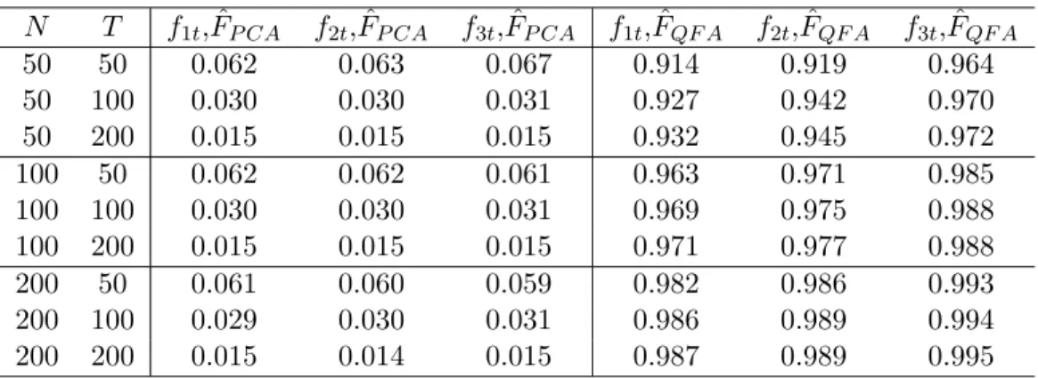
Next, to compare the PCA and QFA estimators of the common factors in the previous DGP, we assume that r = 3 is known. We first get the PCA estimators ˆFP CA, and then obtain the QFA estimator ˆFQF A using the IQR algorithm. Next, we regress each of the true factors on
ˆ
FP CA and ˆFQF A separately, and report the average R2 from 1000 replications in Table 2 as an indicator of how well the space of the true factors is spanned by the estimated factors. As shown in the first three columns of Table 2, while the PCA estimators are not very successful
in capturing the true common factors, our QFA estimators approximate them very well, even when N, T are not too large.
As discussed earlier, the overall findings reported in Tables 1 and 2 are in line with our theoretical results. They provide strong evidence of the substantial gains that can be achieved by using QFA rather than PCA in those cases where the idiosyncratic error terms in AFM exhibit heavy tails and outliers.
5.2 Estimation of QFM: Heavy-tailed and non-independent error terms In this subsection we consider the following DGP:
Xit= 1if1t+ 2if2t+ ( 3if3t)·eit,
wheref1t= 0.8f1,t 1+✏1t,f2t= 0.5f2,t 1+✏2t,f3t=|gt|, 1i, 2i,✏1t,✏2t, gt are all independent draws fromN(0,1), and 3i are independent draws from U[1,2]. FollowingBai and Ng(2002), the following specification foreit is used:
eit= ei,t 1+vit+⇢· i+J X j=i J,j6=i
vjt,
wherevitare independent draws from N(0,1) except in the second case below. The autoregres-sive coefficient captures the serial correlations of eit, while the parameters ⇢ and J capture the cross-sectional correlations of eit. We consider four cases:
Case 1: Independent errors: = 0 and ⇢= 0,
Case 2: Independent errors with heavy tails: =⇢= 0, and vit⇠i.i.dStudent(3). Case 3: Serially Correlated Errors: = 0.2 and⇢= 0.
Case 4: Serially and Cross-Sectionally Correlated Errors: = 0.2 and⇢= 0.2, andJ = 3.
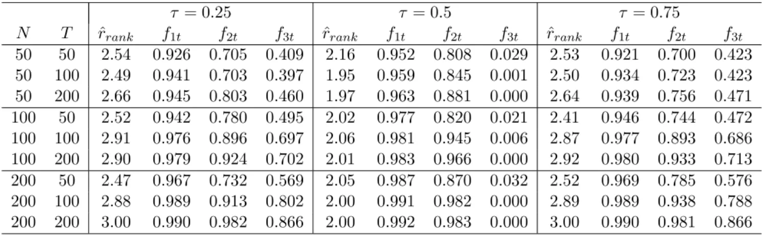
For each of the previous cases and each ⌧ 2 {0.25,0.5,0.75}, we first estimate ˆr using our rank-minimization estimator, having set k and PN T as described in the previous subsection. Second, we estimate ˆr factors by means of the QFA estimation approach, which we denote as ˆFrˆ
QF A. Finally, we regress each of the true factors on ˆFQF Aˆr and calculate the R2s. This procedure is repeated 1000 times and for each⌧, we report the averages of ˆrand theR2s among these 1000 replications.
The results for Case 1 and Case 2 (where this time the heavy tails are captured by a Stu-dent(3) rather than by a Cauchy distribution) are reported in Tables 3 and 4, respectively, for
N, T 2{50,100,200}. Notice that for⌧ = 0.25,0.75, we haver(⌧) = 3 while, for⌧ = 0.5, we get
r(⌧) = 2, since the factorf3tdoes not a↵ect the median ofXit. It can be observed that both our rank-minimization selection criterion and the QFA estimators perform very well in choosing the
true number of QFA factors and in estimating them. It should be noticed that at⌧ = 0.25,0.75 the estimation of the scale factorf3t is not as good as the mean factorsf1t, f2tfor small N and
T. However, such di↵erences vanish asN andT increase.
The results for Case 3 and Case 4 are in turn reported in Tables 5 and 6, respectively. It can be inspected that, even when the independence assumption is violated in these DGPs, the QFA estimation approach still performs satisfactorily. Thus, despite adopting independence in Assumption 1 (iii) for tractability in the proofs (see Remark 1.4), it seems that QFA estimation still works properly when the errors terms are allowed to exhibit mild serial and cross-sectional correlations.
6
Empirical Applications
In this section we illustrate the use of the QFA estimation approach in practice by considering three empirical applications that involve macroeconomic, financial, and climate change data:
1. The first dataset (SW for short) corresponds to an updated version of the popular panel of macroeconomic indicators which has been used by Stock and Watson to construct leading indicators for the US economy. This dataset can be downloaded from Mark Watson’s website. SW consists of 167 quarterly macro-variables from 1959 to 2014 (N = 167, T = 221). These variable are transformed into stationary series before estimating the factors (see Stock and Watson 2016for the details of this dataset).
2. The second dataset (Climate for short) consists of the annual changes of temperature from 338 stations from 1916 to 2016 (N = 338, T = 100) drawn from the Climate Research Unit (CRU) at the University of East Anglia, where information about global temperatures across di↵erent stations in the Northern and Southern Hemisphere is provided.
3. The third dataset (MF for short) contains the monthly returns of 2378 mutual funds from 2000 to 2014 (N = 2378, T = 180), obtained from the Center of Research for Security Prices (CRSP).
First, we set the number of PCA estimated factors in the SW dataset to be equal to 3 since this is the conventional number of factors found in the macroeconomic literature (typically capturing variability in TFP, monetary and fiscal variables). In contrast, for the Climate and MF datasets, which have been less explored in the AFM literature, we use the eigenvalue-ratio estimator ofAhn and Horenstein(2013) which selects 2 and 3 PCA factors, respectively;8 next, we estimate the number of quantile-dependent factors using our rank-minimization estimator at ⌧ = 0.1,0.25,0.5,0.75,0.9.
8We also applied the IC-based method ofBai and Ng (2002), but it was found that this selection procedure
always chooses the maximum number of factors (8) for all the three datasets. For this reason, we only report the results of the eigenvalue-ratio estimator, whose finite-sample performance has been shown byAhn and Horenstein
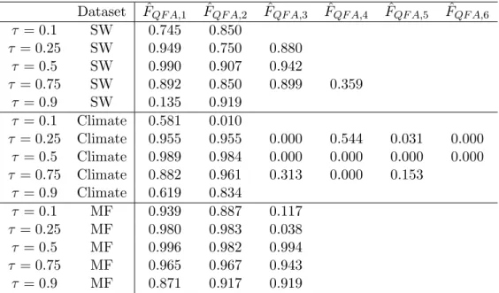
The results of the previous exercise are reported in Table 7. Two di↵erent sets of findings stand out. On the one hand, there are two datasets where the estimated number of PCA and QFA factors across quantiles is quite similar or even identical. The first one is the SW dataset, where the estimated number of QFA factors using our rank-minimization estimator never di↵ers from the estimated number of PCA factors (3) by more than one factor; for example, at⌧ = 0.10 and 0.9, the chosen number of QFA factors is 2 while it is 4 at⌧ = 0.75. In line with the discussion in subsection 3.3, our interpretation of these results is that some of the four selected quantile-varying factors may be relevant at⌧ = 0.75, while they may be weak at the other two quantiles. The second one in this category is the MF dataset, where we find an even stronger degree of similarity between the number of QFA and PCA factors: for all considered⌧s, they are always identical (3).
On the other hand, the evidence for the Climate dataset is rather di↵erent. In e↵ect, with the exception of two tails of the distribution (⌧ = 0.1 and 0.9), where the estimated number of QFA factors equals the number of PCA factors (2), the selected number of QFA factors at the remaining quantiles (5 or 6) is much larger.
Thus, in line with the discussion in subsection 3.3, the previous findings for the Climate dataset strongly indicate that PCA fails to capture all relevant factors in the QFM representa-tion, implying that the QFA estimation approach is required to extract them. Regarding the SW and MF datasets, it was also argued in subsection 3.3 that equality (or similarity) of the number of PCA and QFA factors at all considered ⌧s does not necessarily imply that PCA captures all relevant factors. To check this, we examine the size of the correlation of each QFA factor at each⌧ with the set of estimated PCA factors. If these correlations are high, this would indicate that the QFA factors only capture the PCA factors, with no other extra factors being relevant. Conversely, if the correlations are low at some ⌧, this will indicate the presence of some extra factor at such a⌧ that PCA is unable to uncover.
Following this strategy, Table 8 shows the results of of comparing ˆFF QAwith the PCA factors (denoted as ˆFP CA).9 For each ⌧, we regress each element of ˆFQF A on ˆFP CA, and report the
R2s of these regressions. The main finding is that most of these R2s are close to 1 (which is
not surprising since mean-shifting factors a↵ect most of the quantiles) but with a few noticeable exceptions: (i) the first QFA factor of SW at ⌧ = 0.9, (ii) the two QFA factors of Climate at ⌧ = 0.1 and 0.9, and (iii) the third QFA factor of MF at ⌧ = 0.1 and 0.25. These exceptions indicate that, besides the mean-shifting factors, the QFA estimation procedure is able to uncover other quantile-dependent factors which could provide extra information about the distributional characteristics of the data.
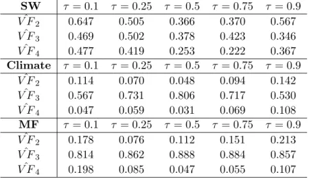
Finally, we further investigate the origins of these extra QFA factors so as to improve their 9As in Table 7, we estimate 3, 2 and 3 mean factors for SW, Climate and MF, respectively, whereas the number
interpretation. We do this by comparing them to the volatility factors obtained by the PCA-SQ procedure, denoted as ˆV F2. The insight for this comparison can be provided by Example 3
above, where the extra QFA factors happen to be volatility factors and hence should be highly correlated. Furthermore, in a similar fashion, we also construct skewness factors and kurtosis
factors by applying PCA to the third and fourth powers of the residuals obtained after removing the PCA factors from the data, which we denote as ˆV F3 and ˆV F4, respectively. Table 9 reports
theR2s of regressing ˆV Fj on ˆFQF A forj= 2,3,4 at di↵erent⌧s. The results for the SW dataset are somewhat mixed. As can be observed in the first three rows of this Table, the explanatory power of the volatility, skewness and kurtosis factors over the QFA factors is fairly moderate. This evidence, together with the strong correlations between the PCA and QFA factors reported in Table 8, seems to point out that the three selected PCA factors play a dominant role in the QFM structure. Yet, in view of the slightly higher correlations (R2s close to or above 0.6) of
the QFA factors with ˆV F2 at the lower and upper quantiles, one cannot rule out that extra
factors related to volatility may still be relevant. By contrast, for Climate and MF, the evidence is much clearer: the skewness factor is highly correlated with the estimated QFA factors at most ⌧s, whereas the volatility and kurtosis factors are not correlated at all with them. This finding points to the existence of common factors related to symmetry in the distribution of the variables included in these two datasets, which are properly captured by means of the QFA estimation procedure but omitted when applying PCA.
Interestingly, the evidence for the MF dataset is in line with the results by Andersen et al. (2018) who report the existence of tail factors in the distribution of asset returns which, for our specific dataset, we interpret as being closely related to changes in skewness. Likewise, the evidence for the Climate dataset is also in line with the results obtained byGadea and Gonzalo (2019). Using the same dataset we use here (but di↵erent quantile techniques), these authors find that global warming over the last century seems to be due to a di↵erent behaviour in the lower tail than in the central and upper tails of the distribution of global temperatures. This finding points to a change in the skewness of such a distribution, in agreement with the nature of the extra QFA factors found for this dataset.
7
Conclusions
Approximate Factor Models (AFM) have become a leading methodology for the joint modelling of large number of economic time series with the big improvements in data collection and infor-mation technologies. This first generation of AFM was designed to reduce the dimensionality of big datasets by finding those common components which, by shifting the means of the observed variables with di↵erent intensities, are able to capture a large fraction of the data co-movements. However, one could envisage the existence of other common factors that do not (or not only)
shift the means but also a↵ect other distributional characteristics (volatility, higher moments, extreme values, etc.). This calls for a second generation of factor models.
Inspired by the generalization of linear regressions to quantile regressions (QR), this paper proposes Quantile Factor Models (QFM) as a new class of factor models. In QFM, both factors and loadings are allowed to be quantile-dependent objects. These extra factors could be useful for identification purposes, for instance mean-shifting factors vs. volatility/skewness/kurtosis factors, as well as for forecasting purposes in factor-augmented regressions and FAVAR setups. Using tools in the interface of QR, Principal Component Analysis (PCA) and the theory of empirical processes, we propose a novel estimation procedure, labelled Quantile Factor Analysis (QFA), that yields consistent and asymptotically normal estimators of factors and loadings at each quantile. An important advantage of QFA is that it is able to extract simultaneously all mean-shifting and extra factors determining the factor structure of QFM, in contrast to PCA which can only extract mean-shifting factors. In addition, we propose two selection criteria to estimate consistently the number of factors at each quantile. Finally, another interesting result is that QFA estimators remain valid when the idiosyncratic error terms in AFM exhibit heavy tails and outliers, which is a case where PCA is rendered invalid.
The previous theoretical findings receive support in finite samples from a range of Monte Carlo simulations. Furthermore, it is shown in these simulations that QFA estimation per-forms well when we depart from some of simplifying assumptions used in the theory section for tractability (like, e.g., independence of the idiosyncratic errors). Lastly, our empirical applica-tions to three large panel datasets of financial, macro and climate variables provide evidence that some these extra factors may be highly relevant in practice.
Any time a novel methodology is proposed, new research issues emerge for future investi-gation. Among the ones which have been left out of this paper (some are part of our current research agenda), four topics stand out as important:
• Factor augmented regressions and FAVAR: In relation to this topic, it would also be interesting to check the contributions of the extra factors in forecasting and monitoring (see, e.g.,Stock and Watson 2002for this type of analysis). This is an issue of high interest for applied researchers, especially with the surge of Big Data technologies. For example, one could analyze the role of the extra factors in the estimation and shock identification in FAVAR. Recent developments in quantile VAR estimation, as in White et al. (2015) provide useful tools in addressing these issues.
• Relaxing the independence assumptions: in view of the simulation results in Tables 5 and 6, we conjecture that the main theoretical results of our paper continue to hold when the error terms in QFM are allowed to have weak cross-sectional and serial dependence. Providing a formal justification for this conjecture remains high in our research agenda. As discussed in Remark 1.4, the goal here is to provide more general conditions on uit
under which the sub-Gaussian type inequalities still hold.
• Dynamic QFM: Although our methodology admits factors to exhibit dependence, provided Assumption 2(i) holds, a pending issue is how to extend our results for static QFM to dynamic QFM, where the set of quantile-dependent objects include lagged factors (see Forni et al. 2000and Stock and Watson 2011). Since our main aim in this paper has been to introduce the new class of QFM and their basic properties, for the sake of brevity, we have focused on static QFM, leaving this topic for further investigation.
• Economic interpretation of QFA factors in empirical applications: given the evidence that extra factors could be relevant in practice, another interesting issue is how to interpret them in di↵erent economic and financial contexts. Once the econometric techniques to detect and estimate extra factors in QFM have been established, attempts to provide new economic insights for these objects would help enrich the economic theory underlying this type of factor structures.
A
Tables and Figures
Table 1: AFM with Cauchy-distributed Error Terms: Number of Factors
N T P Cp1 of BN ICp1 of BN Eigenvalue Ratio Rank Estimator
50 50 [0.0, 0.0, 100] [0.1, 0.2, 99.7] [74.6, 10.5, 14.9] [43.2, 32.5, 24.3] 50 100 [0.0, 0.0, 100] [0.0, 0.2, 99.8] [75.8, 9.9, 14.3] [37.7, 54.9, 7.4] 50 200 [0.0, 0.0, 100] [0.0, 0.1, 99.9] [74.0, 11.3, 14.7] [46.3, 48.1.0, 5.6] 100 50 [0.0, 0.0, 100] [0.0, 0.0, 100] [76.3, 9.7, 14.0] [39.1, 52.0, 8.9] 100 100 [0.0, 0.0, 100] [0.0, 0.0, 100] [75.2, 9.5, 15.3] [8.9, 90.3, 0.9] 100 200 [0.0, 0.0, 100] [0.0, 0.0, 100] [74.1, 11.3, 14.6] [7.4, 92.2, 0.4] 200 50 [0.0, 0.0, 100] [0.0, 0.0, 100] [75.7, 11.4, 12.9] [41.0, 55.2, 3.8] 200 100 [0.0, 0.0, 100] [0.0, 0.0, 100] [74.0, 11.7, 14.3] [7.1, 92.6, 0.3] 200 200 [0.0, 0.0, 100] [0.0, 0.0, 100] [72.4, 11.3, 16.3] [0.0, 100, 0.0] Note: The DGP considered in this Table: Xit = P3j=1 jifjt + uit, where
f1t = 0.2f1,t 1 + ✏1t, f2t = 0.5f2,t 1 + ✏2t, f3t = 0.8f3,t 1 + ✏3t, ji,✏jt ⇠ i.i.dN(0,1), uit ⇠ i.i.dCauchy(0,1). For each estimation method, we reported [proportion of ˆr <3 , proportion of ˆr= 3, proportion of ˆr >3 ] from 1000 replications.
Table 2: AFM with Cauchy-distributed Error Terms: Estimation of Factors
N T f1t, ˆFP CA f2t, ˆFP CA f3t, ˆFP CA f1t, ˆFQF A f2t, ˆFQF A f3t, ˆFQF A 50 50 0.062 0.063 0.067 0.914 0.919 0.964 50 100 0.030 0.030 0.031 0.927 0.942 0.970 50 200 0.015 0.015 0.015 0.932 0.945 0.972 100 50 0.062 0.062 0.061 0.963 0.971 0.985 100 100 0.030 0.030 0.031 0.969 0.975 0.988 100 200 0.015 0.015 0.015 0.971 0.977 0.988 200 50 0.061 0.060 0.059 0.982 0.986 0.993 200 100 0.029 0.030 0.031 0.986 0.989 0.994 200 200 0.015 0.014 0.015 0.987 0.989 0.995
Note: The DGP considered in this Table is: Xit = P3j=1 jifjt+uit, where f1t =
0.2f1,t 1+✏1t, f2t = 0.5f2,t 1+✏2t, f3t = 0.8f3,t 1+✏3t, ji,✏jt ⇠i.i.d N(0,1), uit ⇠ i.i.d Cauchy(0,1). For each estimation method, we report the averageR2in the regression of (each of) the true factors on the estimated factors by PCA and QFA.